A System-Approach for Recoverable Spare Parts Management Using the Discrete Weibull Distribution

Abstract

Optimal spare parts management strategies allow sustaining a system’s availability, while ensuring timely and effective maintenance. Following a systemic perspective, this paper starts from the Multi-Echelon Technique for Recoverable Item Control (METRIC) to investigate the potential use of a Weibull distribution for modelling items’ demand in case of failure. Adapting the analytic formulation of METRIC through a Discrete Weibull distribution, this study originally proposes a METRIC-based model (DW-METRIC) to be used for modelling the stochastic demand in multi-item systems, in order to ensure process sustainability. The DW-METRIC has been tested in a case study related to an industrial plant constituted by 98 items in a passive redundancy configuration. Comparing the results via a simulation model, the outcomes of the study allow defining applicability criteria for the DW-METRIC, in those settings where the DW-METRIC offers more accurate estimations than the traditional METRIC.

1. Introduction

In the current competitive industrial scenario, equipment requires optimum inventory management, especially in those sectors (e.g., aviation, defense, oil and gas, nuclear power plants, etc.) where any failure may have critical consequences on both productivity and safety. Considering the supply chain’s organization of these systems as a complex network structure (multi-echelon) with multiple items related through different levels of the bill of materials (multi-indenture), spare parts require accurate, sustainable and cost-effective management strategies.

Traditionally, an individual optimization approach—item-approach [1]—has been used for optimizing spare parts allocation. However, due to the modern supply chain’s complexity (i.e., high number of items, tight functional inter-relationships, highly-interacting logistic network structure, differentiated maintainability), it has progressively started falling short for modelling real operating conditions. On the other hand, approaches aimed at optimizing the system’s parameters jointly—system-approach [1]—allow for defining an overall cost-availability function, with an increasing interest in a number of industrial case studies. The METRIC (Multi Echelon Technique for Recoverable Item Control) can be considered the most common approach for defining a system-approach optimization process. Starting from a previously published pivotal study [2], the METRIC allows developing a mathematical model of a base-depot supply system. In the METRIC, the item demand assumes Poisson values with a mean value estimated by a Bayesian procedure. The METRIC’s target consists of defining a sustainable solution to optimally allocate spare parts in warehouses at different levels of the logistic network, ensuring minimum holding and backorder cost, subject to an availability constraint. Due to the non-stationarity of item demand in logistic operations [3], a Poisson process does not necessarily model demand behavior accurately. As has emerged in the literature, the traditional Poisson METRIC remains the most used approach, even if there are several alternative distributions proposed to deal with some peculiar demand patterns, (e.g.,) Refs. [4,5,6].

This study aims at further exploiting the mathematical formulation of METRIC, substituting the Poisson pattern with a Weibull distribution, which is largely used in reliability analysis. Even if mathematically it is more complicated, the Weibull distribution may be more appropriate to model items with a low failure rate, as theoretically argued by Sherbrooke himself [1] (p.89). This conceptual approach has not been further exploited in the literature yet, lacking both an analytical formulation and empirical evidence from industrial case studies.

Traditionally, reorder point strategies were used to control and manage spare parts inventories, optimizing the material costs and utilization. For this reason, several inventory management studies have focused on forecasting the time of future failures based on available failure observations [7,8] and addressed the determination of the ordering amount of spares [9]. Nevertheless, an effective model should be able to determine how many spares must be stocked in a warehouse to satisfy systemic availability requirements, while minimizing costs. The model should also support the decision-maker at addressing the relationships between budget allocations and availability requirements. The METRIC has been conceived to support the optimization of stock levels in multi-echelon multi-indenture systems for recoverable items in a (S-1, S) replenishment policy [1]. Adopting a managerial perspective, the METRIC requires simple input variables (e.g., demand values, Ordering Time, Repairing Time, repair time) and constraints (e.g., site or system availability, budget, warehouse available volume) to provide manageable outcomes (stock level for each item, for each site). The relevance of METRIC has been confirmed by a number of applications in a variety of systems, mainly aviation, naval operations and defense, proving that its structure allows for parametric assessment of order costs, stock levels and back-orders [10,11,12,13,14]. Motivated by the large number of industry examples, this paper aims to further investigate the METRIC theory and the usage of Weibull distribution to model item demands. Inspired by the large number of reliability studies adopting the Weibull distribution to model failures, in this research, the Weibull distribution has been exploratively substituted to the traditional Poisson distribution. The Weibull distribution is well-known in the field of failure analysis [15,16,17]. In the literature, it is possible to find applications in formulations aligned with traditional item-approaches, (e.g.,) prediction on the time of future failures [18], or determination of the stock level for a continuous-review system [19]. Nevertheless, for the adoption of Weibull distribution in METRIC to model an item’s demand, it is necessary to refer to a Discrete Weibull distribution, coherent with the physical dimensions of the spares, which assume obviously discrete values. In this paper, the Discrete Weibull introduced by Nakagawa and Osaki [20] has been adopted, which has been used in reliability engineering, because failure data are measured through discrete variables such as cycles, blows, shocks, or revolutions, (e.g.,) Ref. [21,22,23]. The analytical METRIC-based formulation proposed in this paper, i.e., the DW-METRIC, encompasses a Discrete Weibull (DW) distribution to model the item’s pipeline. The results of the DW-METRIC have been compared to real demand patterns (and to METRIC-based estimations) through a simulation approach.

Based on these observations, the objectives of this study are: (i) to develop an optimization METRIC-based model for recoverable spare parts management using a Discrete Weibull distribution for the demand; (ii) to test the results of the model with a traditional Poisson-based METRIC model via a simulation approach; and (iii) to identify decision criteria for the practical adoption of the proposed method.

The remainder of the paper is organized as follows. Section 2 presents the relevant mathematical formulation for the Discrete Weibull process. Section 3 details the proposed method, i.e., the Discrete Weibull METRIC (DW-METRIC). Section 4 clarifies the results of the DW-METRIC in a 98-item case study, with a comparison of the results shown by the traditional METRIC, as further discussed in Section 5. Lastly, the conclusions summarize the outcomes of the proposed approach and pave the way to future research.

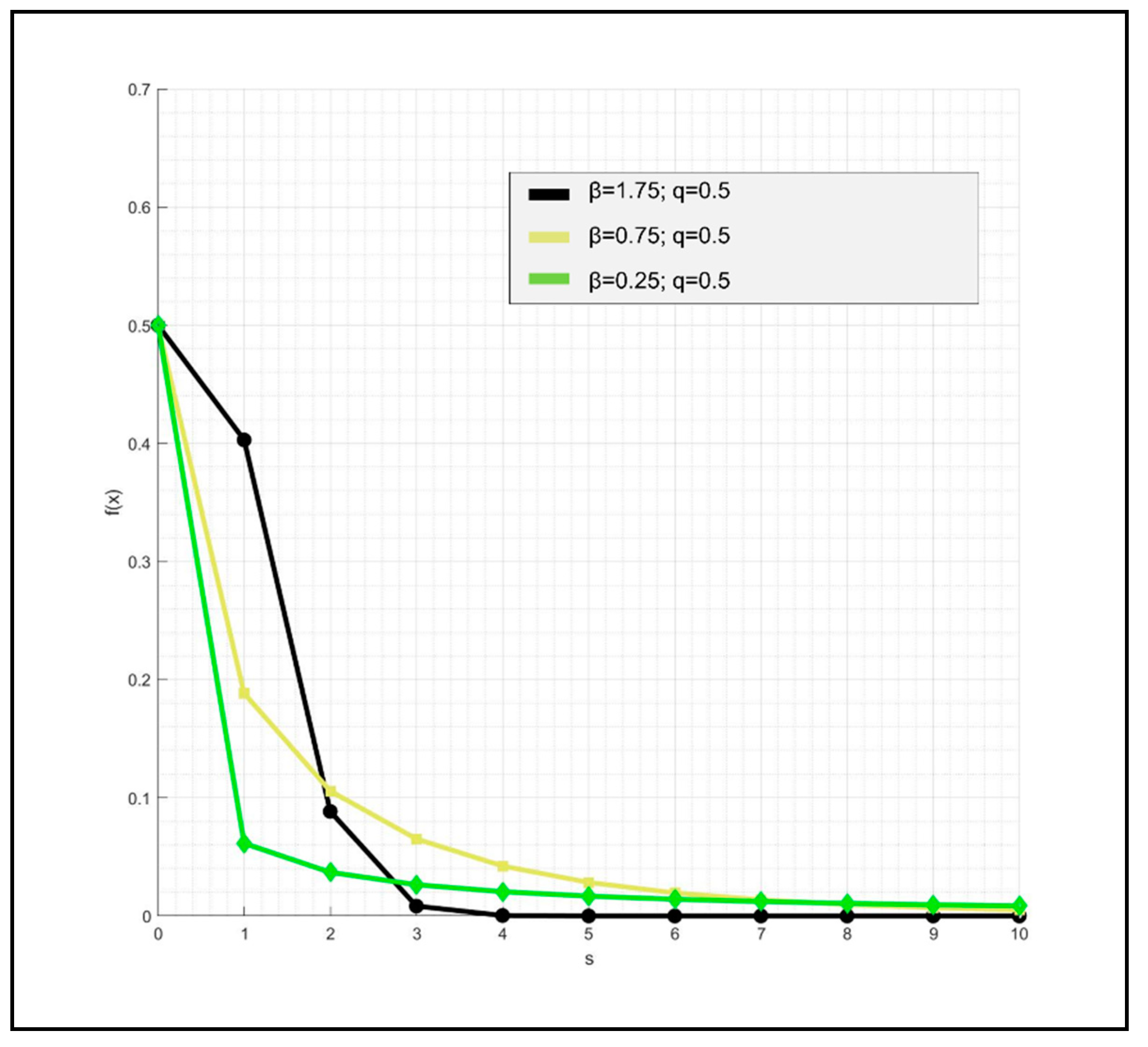
2. Materials and Methods: About the Discrete Weibull Distribution

Parameters

$A_{target}$	Target availability of the system at site
$C_{budget}$	Budget constraint of the system at site
I	Total number of items for each machine in the system
M	Minimum required number of the machines at site
N	Number of the machines at site
$P_i$	Market value of the i-th item
$P_{sw}$	Probability of stand-by switching for a cold machine at site
$T_i$	Repair time at site of the i-th item.

Variables

$\alpha$	Continuous Weibull scale parameter
$\beta$	Standard Discrete Weibull shape parameter
${\beta }_i$	Discrete Weibull shape parameter of the i-th item
${\beta }^{*}$	Estimator of Discrete Weibull shape parameter
${\delta }_i$	Marginal allocation ability gene of the i-th item
$\Delta EB{O}_P$	Difference between analytic and simulated Expected Backorder for METRIC
$\Delta EB{O}_{DW}$	Difference between analytic and simulated Expected Backorder for DW-METRIC
$A$	Machine availability at site
$A_i$	Availability of the i-th item at site
$A_{SYS}$	Availability of the system
$B{O}_i$	Number of $LR{U}_i$ in back order of the i-th item because of a stock-out at site
$D{I}_i$	Number of $LR{U}_i$ of the i-th item Due-In from repair at site
$E_i\left[X\right]$	Expected value of the Discrete Weibull distribution for the ith item
$EB{O}_i\left(s_i\right)$	Expected Backorder for the i-th item at site, with respect to stock level $s_i$
$EBO{*}_i\left(s_i\right)$	Simulated backorder for the i-th item at site, with respect to stock level $s_i$
$F\left(x\right)$	Discrete Weibull cumulative distribution function
$K$	Integer number for the estimation of Discrete Weibull’s mean value
$O{H}_i$	Number of $LR{U}_i$ on hand of the i-th item, i.e., currently available at site
$S\left(x\right)$	Continuous Weibull cumulative distribution function
$I\left(x_i\right)$	Indicator function for the random variable $x_i$ for the method of proportions
$Y$	Total number of zeros (0) in the sample
$Z$	Total number of ones (1) in the sample
$d_i^t$	Weekly demand of item i-th at time t
$f\left(x\right)$	Discrete Weibull probability function
$f_i\left(x\right)$	Probability distribution of x-th stock Due-In, from repair of the i-th item at site
i	Item number, $i=1,\dots ,I$
$m_i$	Yearly demand mean value of the i-th item
n	Total number of observations for a sample demand
$p\left(0\right)$	Probability distribution of zeros in the sample demand
$p\left(1\right)$	Probability distribution of ones in the sample demand
$q$	Standard Discrete Weibull scale parameter
$q_i$	Discrete Weibull scale parameter of the i-th item
$q^{*}$	Estimator of Discrete Weibull scale parameter
$s$	Array of stock level for each item at site, $s=\left(s_1,\dots ,s_I\right)$
$s_i$	Stock level of the i-th item at site

From the pivotal work of Nakagawa and Osaki [20], the Discrete Weibull (DW) is defined to correspond with the continuous Weibull distribution. The respective probability mass function (pmf) can be expressed as follows (1):

$$f\left(x\right)=q^{x^{\beta }}-q^{{(x+1)}^{\beta }}\{\begin{array}{c}0<q<1,\\ \beta >0,\\ x=0,1,2,\dots ,\infty \end{array}$$

(1)

Where:

• $q$ is the scale parameter
• $\beta$ is the shape parameter
• $\beta$ is supposed to be the same one as the continuous Weibull distribution [24]. The cumulative distribution function is defined as [25]:

  $$F\left(x\right)=1-q^{x^{\beta }}$$

  (2)

A way to compute $q$ and $\beta$ is to use the existing relationship between the Discrete Weibull parameters and the continuous ones, see Refs. [20,24]. In detail, the cumulative distribution function (2) is obtained from the survival function of continuous Weibull (3), replacing the exponential term in (3) by a different parameter that is $q$:

$$S\left(x\right)=1-e^{-\left[{\left(\frac{x}{\alpha }\right)}^{\beta }\right]}\{\begin{array}{c}\alpha >0,\\ \beta >0,\\ x\in \left(0,+\infty \right)\end{array}$$

(3)

$$q=e^{-\left(\frac{1}{\alpha }\right)}$$

(4)

For estimating the parameters of the Discrete Weibull, it would be possible to apply the maximum likelihood estimator (MLE) method [26]. Nevertheless, since the value zero is not defined for a random continuous Weibull variable, the MLE method remains inapplicable in the case of a dataset which includes null value(s), i.e., null demand in a time period. Such a restriction can be critical for the applicability of the proposed model, especially for high-availability items, which are subject to low failure rate.

Nevertheless, it is possible to find several Discrete Weibull parameters estimation methods, like the method of moments [24] and MLE for Discrete Weibull [27]. However, since the respective analytical formulations include infinite series, they cannot be solved by ordinary techniques. To overcome this limitation, an efficient method to estimate $q$ and $\beta$, the so-called method of proportions is presented [24], which is here preferred to reduce computational and analytical efforts in evolving the METRIC formulation.

2.1. Method of Proportions

Let $x_1,x_2,\dots ,x_n$ be a random sample from the distribution with pmf given by (1). Firstly, it is necessary to define the indicator function $I\left(x_i\right)$ (5):

$$I\left(x_i\right)=\{\begin{array}{c}1if{x}_i=0\\ 0if{x}_i>0\end{array}$$

(5)

Secondly, $Y$ is computed as the total number of zeros in the sample (6):

$$Y={\displaystyle \sum }_{i=1}^{n}I\left(x_i\right)$$

(6)

The proportion Y/n estimates the probability that the random variable of the distribution assumes the null value (7):

$$p\left(0\right)=Y/n$$

(7)

Considering $q^{*}$ as an empirical estimate of $\mathrm{Pr}\{x>0\}$ and consistent estimator of $q$, $q^{*}$ can be defined as follows (8):

$$q^{*}=1-Y/n$$

(8)

Similarly, the probability $p\left(1\right)$ is estimated by the proportion Z/n, where Z denotes the total number of ones in the sample (9).

$$p\left(1\right)=Z/n$$

(9)

Consequently, $\beta$ is expressed as (10) and can be estimated by (11):

$$\beta =\frac{ln\left\{\frac{ln\left(Pr\{X>2\}\right)}{ln\left(Pr\left\{X>l\right\}\right)}\right\}}{ln2}$$

(10)

$${\beta }^{*}=\frac{ln\left\{\frac{ln\left(q-\frac{Z}{n}\right)}{lnq}\right\}}{ln2}$$

(11)

Since $q^{*}$ and ${\beta }^{*}$ share the main properties of their respective values $q$ and $\beta$, they are consistent estimators, and thus, can be used for modelling the Discrete Weibull distribution.

3. Materials and Methods: DW-METRIC

This section details the analytical formulation to be used for introducing the Discrete Weibull into the METRIC, i.e., for generating the DW-METRIC. Adopting the general assumptions of basic METRIC theory, the proposed formulation was analytically contextualized in a single-site single-indenture multi-item system, in order to clarify the mathematical procedure. In line with traditional METRIC theory [1], an (S-1, S) policy is considered appropriate for each item at each level; and any item in a site is always repaired when there is the capability of doing it. Lateral supply is not taken into account.

3.1. Single Site Model

The assumptions for single site systems used for both the analytical formulation and the case studies can be summarized as follows (see also Figure 1). Note that LRU (line replaceable unit) is used to refer to items at the first level of indenture (single-indenture model), in line with inventory management terminology.

-

There is only one site, with its own inventory of spare items and its own workshop

-

There is only one organization level (single-echelon)

-

There are I > 1 different $LRUs$, $LR{U}_1$,…., $LR{U}_I$ (multi-item)

-

The failure of a specific $LR{U}_i$ happens independently of any other $LR{U}_j$ functioning state

-

An infinite repair capacity is assumed for each item at the site

-

The repair time for $LR{U}_i$ are independent and equally-distributed stochastic variables with expected value $T_i$

3.2. Mathematical Formulation

The stock level $s_i$ represents the number of $LR{U}_i$ in the inventory when there is no defect $LR{U}_i$ in the workshop. At a randomly chosen time, the expression of $s_i$ must consider any situation where there are units undergoing repair, which results in less than $s_i$ on the shelf. Furthermore, when no units are on the shelf, any request generates a backorder. The stock balance assumes the generic expression (12):

$$s=\left(s_1,s_2,s_3\dots ,s_I\right)$$

(12)

and, in detail (13):

$$s_i=D{I}_i+O{H}_i-B{O}_i$$

(13)

where:

• $s_i$ represents the number of spare parts of $LR{U}_i$ in the site;
• $O{H}_i$ is the number of units on hand $O{H}_i$, i.e., spare parts currently available in the site;
• $D{I}_i$ is the number of units of stock Due In in base repair;
• $B{O}_i$ (BackOrders) is the number of stocks that is requested but not available on the shelf because of a stock-out.

The variables in (13) can only acquire non-negative integer values, and thus, at each time, at least one of $B{O}_i$ and $O{H}_i$ is zero:

$$B{O}_i={\left(D{I}_i-s_i\right)}^{+}=max\left\{0,D{I}_i-s_i\right\}$$

(14)

$$O{H}_i={\left(s_i-D{I}_i\right)}^{+}=max\left\{0,s_i-D{I}_i\right\}$$

(15)

The expected value of backorders for the i-th $LRU$ can be estimated by (16):

$$EB{O}_i\left(s_i\right)=E\left[B{O}_i\right]=E\left[{\left(D{I}_i-s_i\right)}^{+}\right]$$

(16)

Specifying (16), $EB{O}_i\left(s_i\right)$ can be calculated as (17):

$$EB{O}_i\left(s_i\right)={\displaystyle \sum }_{x=s_i+1}^{\infty }\left(x-s_i\right)f_i\left(x\right)$$

(17)

Further expanding (17), it is possible to write (18):

$${\displaystyle \sum }_{x=s_i+1}^{\infty }\left(x-s_i\right)f_i\left(x\right)={\displaystyle \sum }_{x=s_i+1}^{\infty }x{f}_i\left(x\right)-s_i{\displaystyle \sum }_{x=s_i+1}^{\infty }{f}_i\left(x\right)$$

(18)

where the first term of (18) is (19):

$${\displaystyle \sum }_{x=s_i+1}^{\infty }x{f}_i\left(x\right)={\displaystyle \sum }_{x=0}^{\infty }x{f}_i\left(x\right)-{\displaystyle \sum }_{x=0}^{s_i}x{f}_i\left(x\right)$$

(19)

and the second term of (18) can be written as follows (20):

$$s_i{\displaystyle \sum }_{x=s+1}^{\infty }{f}_i\left(x\right)=s_i\left(1-{\displaystyle \sum }_{x=0}^s{f}_i\left(x\right)\right)$$

(20)

Eventually, the expression of (17), taking into account (1), can be written as (21):

$$EB{O}_i\left(s_i\right)={\displaystyle \sum }_{x=0}^{\infty }x\left(q_i^{x^{{\beta }_i}}-q_i^{{(x+1)}^{{\beta }_i}}\right)-{\displaystyle \sum }_{x=0}^{s_i}x\left(q_i^{x^{{\beta }_i}}-q_i^{{(x+1)}^{{\beta }_i}}\right)-s_i{q}_i^{{\left(s_i+1\right)}^{{\beta }_i}}$$

(21)

The first term on the right side of (21) is the expected value of the Discrete Weibull distribution for the i-th item (22):

$$E_i\left[X\right]={\displaystyle \sum }_{x=0}^{\infty }x\left(q_i^{x^{{\beta }_i}}-q_i^{{(x+1)}^{{\beta }_i}}\right)$$

(22)

where x represents the Discrete random variable of the distribution. Furthermore, for estimating the mean value, it is necessary to update the formulation by [20] (23):

$$E\left[X\right]={\displaystyle \sum }_{x=0}^{\infty }{q}^{x^{\beta }}$$

(23)

which has been corrected by Englehardt & Li [25] (24):

$$\begin{gathered} {\displaystyle \sum }_{x=0}^{\infty }x(q^{x^{\beta }}-q^{{(x+1)}^{\beta }})= \\ =0+1q^{1^{\beta }}+2q^{2^{\beta }}+3q^{3^{\beta }}+4q^{4^{\beta }}\mathrm{..}-0-1q^{2^{\beta }}-2q^{3^{\beta }}-3q^{4^{\beta }}\dots = \\ ={\displaystyle \sum }_{x=1}^{\infty }{q}^{x^{\beta }} \end{gathered}$$

(24)

Nevertheless, (24) cannot be written in a closed form but it can be computed as (25):

$$E\left[X\right]\cong {\displaystyle \sum }_{x=1}^K{q}^{x^{\beta }}+{{\displaystyle \int }}_{K+1}^{\infty }{q}^{x^{\beta }}dx$$

(25)

where K is a large integer value [25].

The second term of (25) can be computed by applying the incomplete gamma function (26):

$${{\displaystyle \int }}_{K+1}^{\infty }{q}^{x^{\beta }}dx=\frac{\Gamma \left[\frac{1}{\beta },{\left(K+1\right)}^{\beta }(-\ln q)\right]}{\beta {\left(-\ln q\right)}^{\frac{1}{\beta }}}$$

(26)

where, observing that for $s_i=0$ $EB{O}_i\left(s_i=0\right)$, (17) becomes (27):

$$EB{O}_i\left(s_i=0\right)=E_i\left[{\left(D{I}_i-s_i\right)}^{+}\right]=E_i\left[X\right]$$

(27)

Equation (27) implies that for null stock, the Expected Backorder for the i-th item is equal to the expected value of the Discrete Weibull distribution. Such a demonstration supports the standard iterative calculation of the distribution’s parameters, as for METRIC formulation [6].

Finally, the total Expected Backorders for a number I of $LR{U}_i$ can be expressed by (28):

$$EBO\left(s\right)={\displaystyle \sum }_{i=1}^{I}EB{O}_i\left(s_i\right)$$

(28)

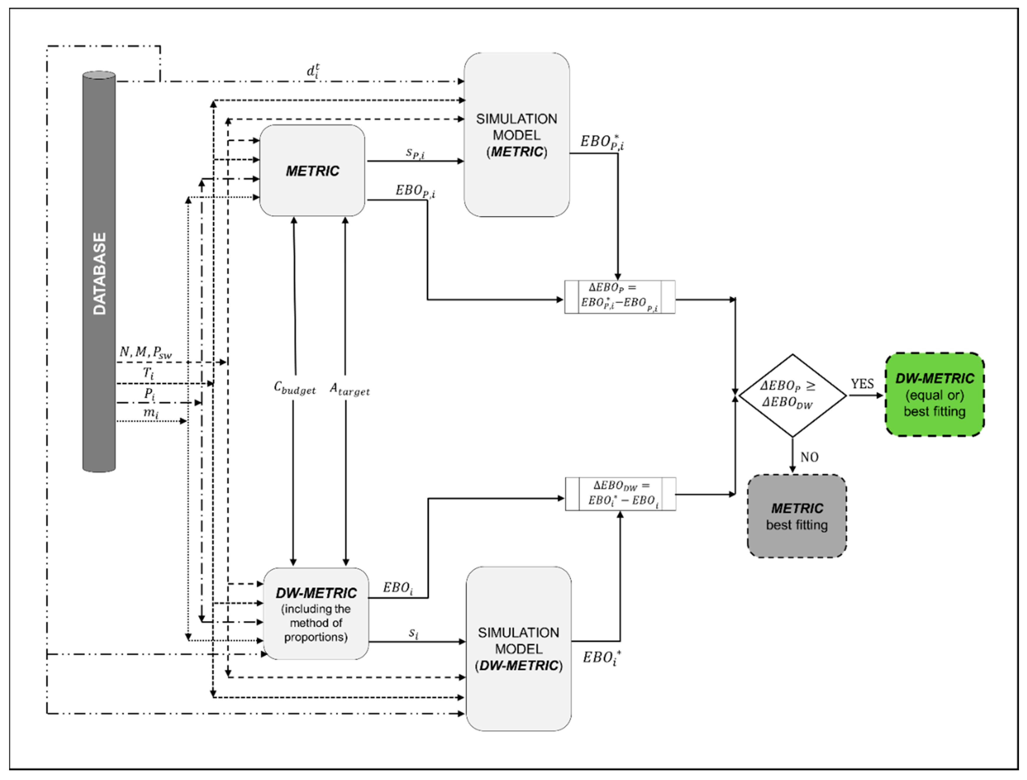
3.3. Optimization Process

The principal objective of the optimization process in METRIC is to compute the optimal stock level $s^{*}=\left(s_1^{*},\dots ,s_I^{*}\right)$ for a group of $LRUs$ at a site that satisfies a target value of system availability. This target is achieved developing an availability versus backorders curve that shows the system’s availability as a function of the expected backorders of the LRUs. This approach is valid since the minimization of the sum of the backorders on all items is equivalent to maximizing the system availability. Analytically, it is necessary to firstly evaluate the availability for each $LR{U}_i$ at site as (29):

$$A_i=\left(1-\frac{EB{O}_i\left(s_i\right)}{N}\right)$$

(29)

where N indicates the number of machines at the site; and the following mathematical constraint (30) has to be valid to make the availability values significant:

$$EB{O}_i\left(s_i\right)\le N$$

(30)

The individual machine availability A can be evaluated as (31), on the simplified assumption of a series system for all the I $LRUs$:

$$A={\displaystyle \prod }_{i=1}^I{A}_i$$

(31)

Assuming that the site has a minimum required number of machines, a failure on a machine reduces the availability of the system only when the number of available machines is lower than the minimum required M. In the case of passive redundancy of the machines, the system availability can be modelled by a redundant system with ($N-M$) stand-by machines, in which M of N must be operating (32):

$$A_{SYS}=A^M\left(1+P_{sw}{\displaystyle \sum }_{k=0}^{N-M}\frac{{\left[-ln{A}^M\right]}^k}{k!}\right)$$

(32)

where A is the equipment availability and $P_{sw}$ is the probability to successfully use one of the cold stand-by equipment. $P_{sw}$ is less than one in order to model an imperfect switching action (e.g., due to overlapping maintenance plans), but it is generally high ($P_{switch}$ equal to, or greater than 0.8) [14].

At this step it is possible to define the optimal stock allocation by the adoption of a marginal allocation algorithm, as usually done for the METRIC [1]. Since the marginal analysis is based on a heuristic, it offers an approximate solution (potentially, a local minimum), which, however, has been confirmed to be reasonably accurate for the type of problems at hand [28,29]. The algorithm starts from an initial condition of null stock for each item and iterates a marginal (one piece more) allocation with the objective of finding the optimal level of the stock that satisfies the system availability constraint, defined by (33):

$$A_{SYS}\ge A_{target}$$

(33)

For each iteration, the heuristic iterates testing the I possible allocations of a new item at site. The algorithm relies on a marginal ability gene ${\delta }_i$ (34) that considers the marginal benefit to add one item to the stock in the i-th position:

$${\delta }_i=\frac{EBO\left(s_i\right)-EBO\left(s_i+1\right)}{P_i}$$

(34)

In (34), ${\delta }_i$ represents the reduction of the system’s Expected Backorder due to the increase of one unit in stock of the i-th item, in relation to its market value. If the allocation does not satisfy the cost constraint, the algorithm rejects the allocation and the second best is tested. Only when the availability constraint (33) is satisfied, the marginal analysis allocates in stock the selected item and then it checks $A_{SYS}$, otherwise the algorithm continues iterating to find a feasible point.

4. Results

This section illustrates the application of the DW-METRIC in an illustrative case study to ensure a sustainable spare parts allocation for an industrial plant.

4.1. Description of the Scenario

The problem refers to spare parts management in a hypothetical industrial plant for hydraulic coal transport, whose functioning requires N = 35 pumping stations, while the items correspond to different $LRUs$ of the pumping station (e.g.,: pump, feed tank, heat exchanger, pipe, differential pressure gauge, sedimentation tank, etc.). The system can be modelled as a single-site, with a dedicated inventory to be optimized and a workshop capable of repairing the defect units. The optimal stock levels have to satisfy the target value of the system availability, $A_{target}=0.97$. Adopting the DW-METRIC and optimizing the model through a marginal allocation algorithm, this section details the optimal stock found by the DW-METRIC, then comparing the results with a traditional Poisson-based METRIC. The system availability is modelled by a passive redundant system with three stand-by machines, i.e., the number of contemporarily required pumps has to be greater or equal to M = 32. The value of $P_{sw}$ represents the probability to use one of the cold pumping stations as a stand-by station if successfully reassigned, and it is assumed to be 0.91, based on previous experience in plant maintenance processes. These input parameters are summarily listed in

Table 1. Input parameters for the model.

Parameter	Value
N	35
M	32
${\mathit{P}}_{\mathit{s}\mathit{w}}$	0.91
I	98
${\mathit{A}}_{\mathit{t}\mathit{a}\mathit{r}\mathit{g}\mathit{e}\mathit{t}}$	0.97
${\mathit{C}}_{\mathit{b}\mathit{u}\mathit{d}\mathit{g}\mathit{e}\mathit{t}}$	$20,000,000

.

The database used for the analysis consists of a monthly demand trend of 98 $LRUs$ (Table 1).

4.2. Application Steps of the DW-METRIC

The application of DW-METRIC in the case study at hand can be briefly summarized into four fundamental steps:

(1)

Demand clustering based on $T_i$.

Adapting the Palm theorem, the items demand patterns for each item $d_i^t$ are firstly clustered in $T_i$, with the purpose of estimating how many requests might contemporarily arrive to the workshop and thus could generate queues.

(2)

Estimation of Discrete Weibull parameters $q$ and $\beta$.

Starting from the clustered data, the Discrete Weibull distribution parameters, i.e.,$q_i$ and ${\beta }_i$, have been estimated through the method of proportions (see Section 2.1).

(3)

Computation of the expected backorder for all LRUs.

An estimation of the expected value has been done following the formulation described in (25). To guarantee the effectiveness of this estimation, Englehardt & Li [25] proposed K = 1000, which is generally much higher than the stock level that is expected for the system at hand (average annual demand 11.9 ± 2.5 piece/year). As a consequence, for the case study at hand, the second term of (25) can be neglected, allowing the following approximation (35):

$$E_i\left[X\right]\cong {\displaystyle \sum }_{x=1}^K{q}_i^{x^{{\beta }_i}}$$

(35)

Eventually, the expression of EBO (21) becomes (36):

$$EB{O}_i\left(s_i\right)={\displaystyle \sum }_{x=1}^M{q}_i^{x^{{\beta }_i}}-{\displaystyle \sum }_{x=0}^{s_i}x\left(q^{x^{{\beta }_i}}-q^{{(x+1)}^{{\beta }_i}}\right)-s_i{q}_i^{{\left(s_i+1\right)}^{{\beta }_i}}$$

(36)

(4)

Optimization process.

The marginal allocation heuristic originally developed in MATLAB has been used to compute the optimal stock allocations. The input data for the METRIC are the system parameters in Table 1, the repair time $T_i$ of $LRUs$, and the Discrete Weibull parameters $q_i$ and ${\beta }_i$. The algorithm computes the expected backorders based on the best stock allocations of each $LRU$: a higher contribution to decreasing the expected backorder, compared to the cost required to achieve the result. The heuristic stops only when the system availability has attained the target value $A_{target}$, and if respecting the $C_{budget}$. The outcomes of the METRIC optimization process are the optimum stock allocations $s^{*}=\left(s_i^{*}\right)$, which satisfies the availability constraint $A_{target}$ and the budget constraint $C_{budget}$.

4.3. Simulation Model

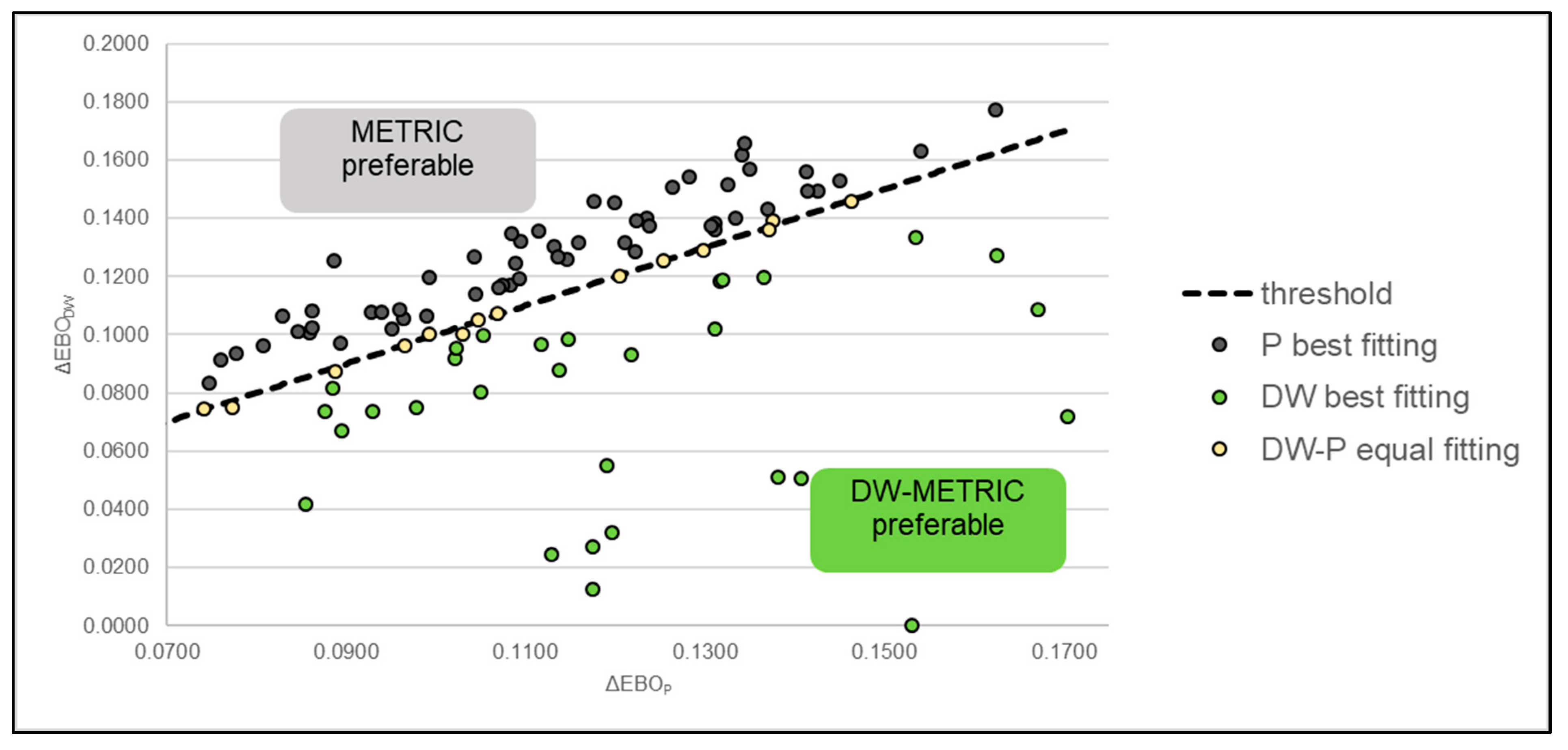
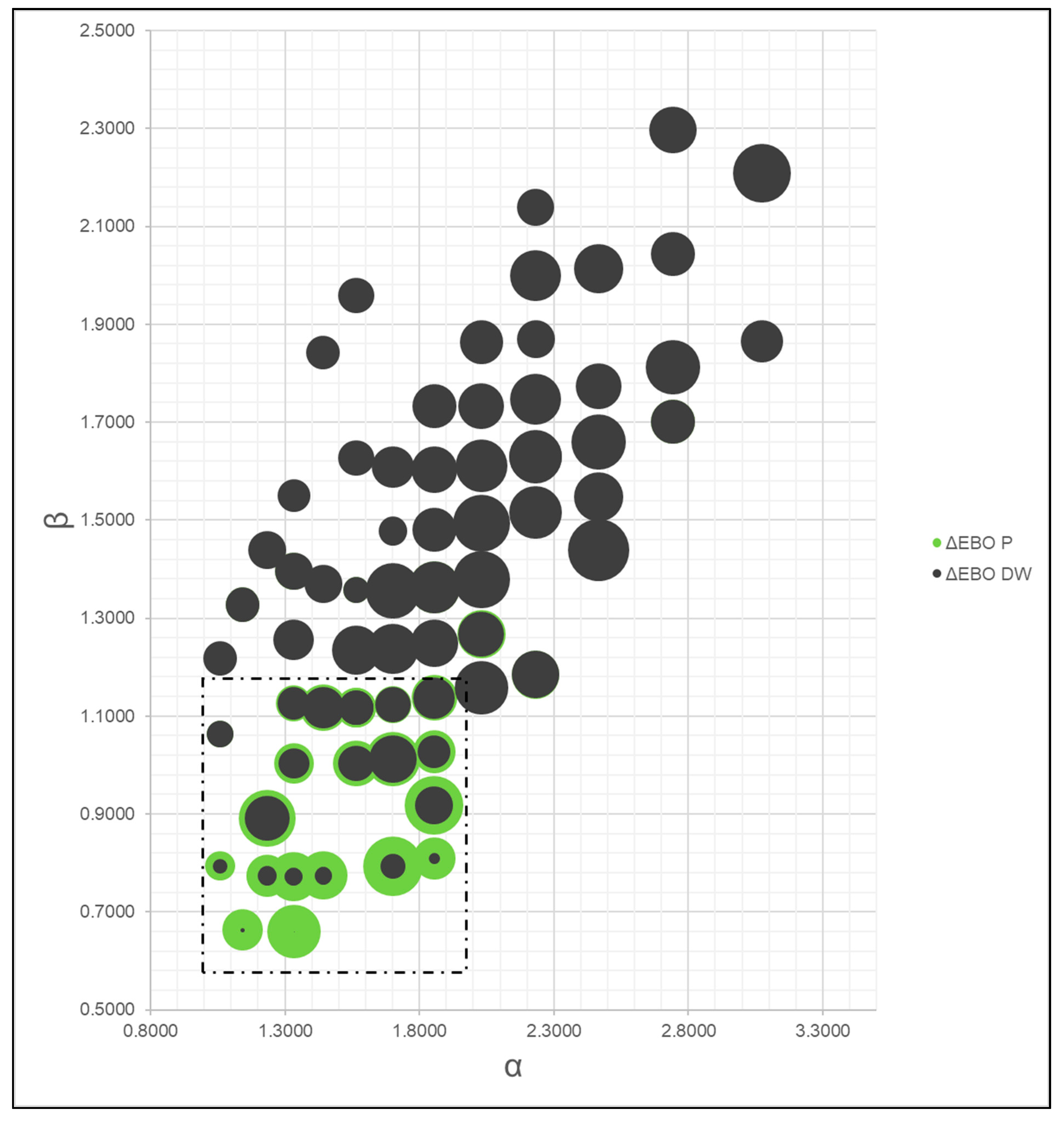
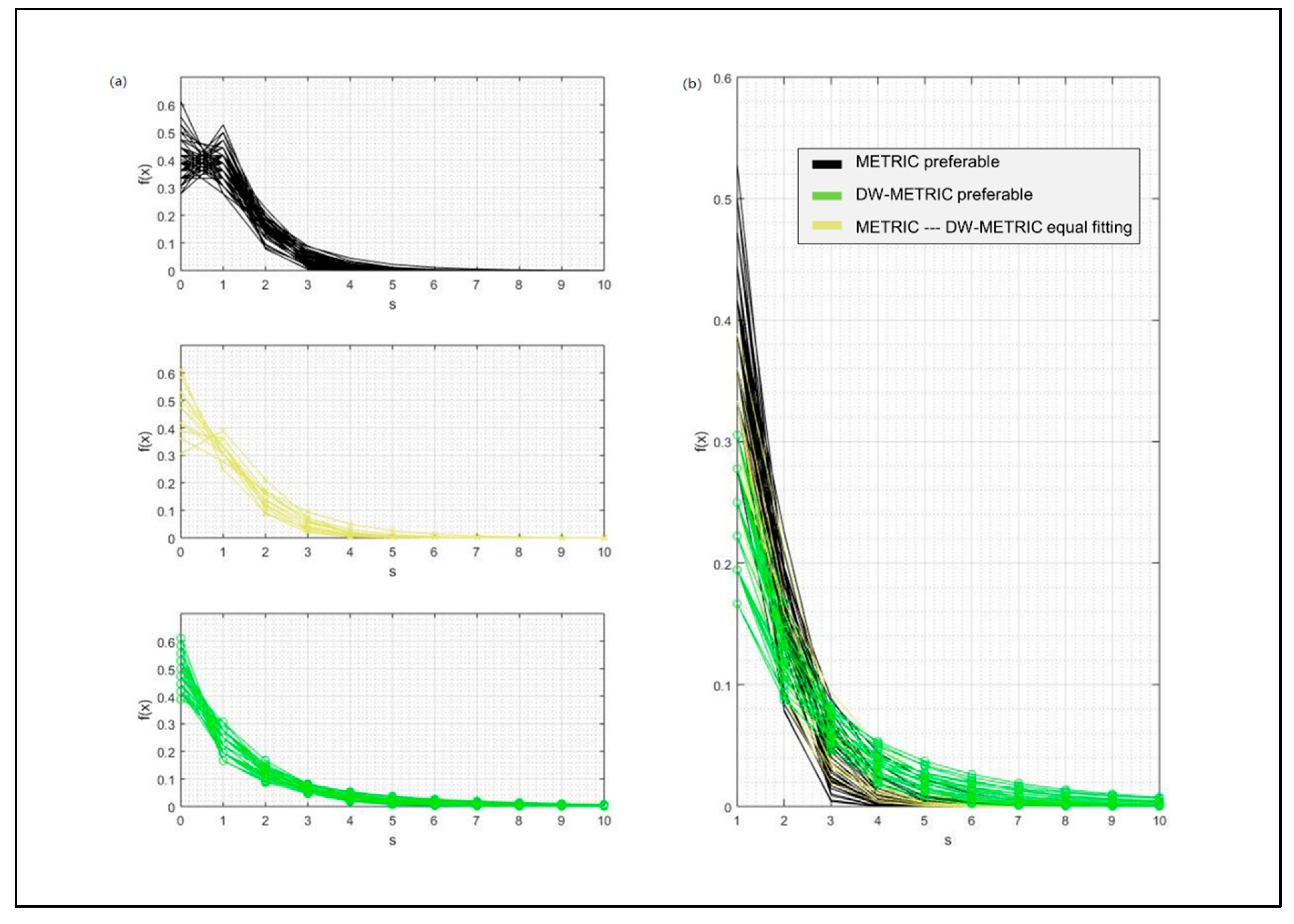
The results have been verified through a simulation model, developed in MATLAB. The simulation model aims at calculating the actual number of Back Orders (BOs), by means of the demand dataset, and by a week-by-week calculation of relevant inventory variables, following the simple logic summarized in (13). The purpose of this phase is understanding whether the DW-METRIC may actually be more accurate than the traditional Poisson-based METRIC. Such an analysis is delivered comparing the EBO estimated by the analytic model with the actual EBO calculated by the simulation model (and as such, being a BO), as shown in Figure 2. Operationally, the input variables and parameters for the simulation model are the proposed optimum stock level $s^{*}$, the repair times ($T_i)$, the cost of the spare ($P_i)$, and other system parameters (M, N, $P_{sw}$, as included in Table 1). Note that the METRIC needs only the average value of demand $m_i$, while the DW-METRIC required the historic demands pattern of each item $d_i^t$, from which we can calculate the DW parameters (${\beta }_i$ and $q_i$, by using the method of proportions, cf. Section 2.1). Both the simulation models inherently require $d_i^t$. The total number of evaluated t time intervals is 144 weeks, i.e., 36 months (3 years). For the sake of representation, the output variables of METRIC and its simulation model are respectively addressed as $s_{P,i}^{ }$ $EB{O}_{P,i}^{}$ $EB{O}_{P,i}^{ *}$, where the subscript P stands for Poisson distribution (referring to traditional METRIC).

5. Discussion

The results of the joint analytical/simulative analysis sketched in Figure 2 are summarized in Figure 3, where the 98 LRUs of the pumping stations are represented as dots colored differently according to the best fitting model: black dots, P, for METRIC; green dots, DW, for DW-METRIC; and yellow, DW-P, for equally fitting. In Figure 3, the threshold represents the bisector of the $\left(\Delta EB{O}_P-\Delta EB{O}_{DW}\right)$ plane: Above the threshold it is possible to find the items for which the traditional METRIC is preferable, and below it, the ones for which DW-METRIC is preferable. The items lying on the threshold present the same errors regardless of the analytic approach (i.e., the two models assign the same stock levels).

One subsequent point of the analysis is related to exploring analytical parameters of items and identifying potential thresholds of applicability for the DW-METRIC. After multiple analyses which aimed at classifying the demand patterns through different variables, an interesting result is represented in Figure 4. Figure 4 summarizes the 98 LRUs in an $\left(\alpha -\beta \right)$ plane, where the bubble size is related to the respective differences between the analytic and simulated EBO (green bubble for $\Delta EB{O}_P$, and black bubble for $\Delta EB{O}_{DW}$). This representation allows depicting those items for which the DW-METRIC is preferable (green bubble visible means that $\Delta EB{O}_P$ is larger than $\Delta EB{O}_{DW}$, and thus DW-METRIC is less biased than METRIC) and vice versa. As such, it is interesting to note that for the items with lower $\beta$ (and $\alpha$ as well, but limited in scope) values, DW-METRIC is certainly preferred.

It could be interesting to further explore the representation of the Discrete Weibull functions for the 98 LRUs, based on the best fitting model (Figure 5a). The joint representation (Figure 5b) provides further evidence of the applicability of DW-METRIC for those items with lower $\beta$ values: The lower the $\beta$, the higher is the variability in the variable of the distribution (i.e., in the item demand), also confirming a general tendency of the item to be characterized by rare failures ($\beta$ remains generally low). For the sake of clarity, the same logic is represented for a single item in Figure 6.

It could also be possible to argue further that the most precise results are related to $\beta <1$, ideally showing that the DW-METRIC would be preferred for those items usually characterized by “infantile failures”, or (in case of $\beta$ approximately equal to 1) for items with random failures. Even if the 98 items in the sample provided too basic knowledge to start assuming such behaviors, these hypotheses, as well as further classifications of demand based on the values of $\alpha$, should be grounded on bigger samples.

6. Conclusions

Starting from the large applications of Weibull distribution in reliability engineering, this paper presents the results of substituting the Poisson distribution for the pipeline with a Discrete Weibull distribution. The outcomes of this research demonstrate that traditional METRIC models based on Poisson distributions do not necessarily represent the best modelling framework for some types of demand patterns. This result has been achieved comparing the outcome of the traditional analytic METRIC, and of an innovative METRIC based on Discrete Weibull distribution (DW-METRIC) via a simulation model. The analyses have been conducted in an industrial plant scenario, constituted by 35 pumping stations, with 98 LRUs each.

Nevertheless, to overcome the limitations for estimating the parameters of the Discrete Weibull distribution in the case of zero values in the variable (i.e., the item demand), this research creatively adopts the method of proportions, which allows for a simple integration into the traditional METRIC. The main outcome of this paper consists of the development of an operational analytic model for system-wide optimization of spare parts, i.e., the DW-METRIC. The results of its application in an industrial context prove that for certain combinations of values in the variables defining the Discrete Weibull distribution $\left(\alpha -\beta \right)$, the DW-METRIC outperforms the METRIC. Even if these results do not cover all the possible combinations of $\left(\alpha -\beta \right)$, it is worthy observing how for lower $\beta$ values $(\beta <1.2)$, the DW-METRIC is generally performing better than the METRIC. This result, which shall be further explored with different databases, is aligned with the limitations of Poisson distribution to capture highly variable demand patterns. The most important research direction shall focus on larger applications to verify the generalizability of the applicability thresholds and their validity to ensure parametric sustainable solutions. A frank consideration about the proposed model refers to its simple structure, i.e., single-site single-indenture. Advancing this originally presented an analytic formulation; the model should be validated for more complex networks, (e.g.,) multi-echelon, multi-indenture, also introducing more complex variables, (e.g.,) cannibalization, alternative redundancy, and routing strategies. Note that limited attention has been devoted to cost estimation, since in this phase, the purpose of the paper consisted of defining the model and proving its effectiveness with respect to METRIC, correctly estimating backorders and availability in operating scenarios. When adding a cost analysis, it could be thus beneficial to refine the optimization strategy with more advanced approaches, (e.g.,) genetic algorithm, pattern search, and particle swarm optimization. In this way, the risk of under-stocking or over-stocking could be assessed more precisely, adding a quantitative dimension of the estimation’s error referring to the different algorithms.

As a long-term research path, this paper also highlights the benefits which should arise from a multi-method comparison, i.e., exploring the threshold of applicability for a series of METRIC-like models, (e.g.,) VARI-METRIC, MOD-METRIC, ZIP-METRIC, in order to guide a priori analysts and researchers in selecting and developing the most suitable expert system for the system being analyzed.

References

1. Sherbrooke, C.C. Optimal Inventory Modeling of Systems: Multi-Echelon Techniques; Springer: Berlin, Germany, 2004; ISBN 1-4020-7849-8. [Google Scholar]
2. Sherbrooke, C.C. Metric: A Multi-Echelon Technique for Recoverable Item Control; Rand: Santa Monica, CA, USA, 1968. [Google Scholar]
3. Sanchez-Rodrigues, V.; Potter, A.; Naim, M.M. Evaluating the causes of uncertainty in logistics operations. Int. J. Logist. Manag. 2010, 21, 45–64. [Google Scholar] [CrossRef]
4. Hillestad, R.J.; Carrillo, M.J. Models and Techniques for Recoverable Item Stockage when Demand and the Repair Process Are Nonstationary—Part I: Performance Measurement; Rand: Santa Monica, CA, USA, 1980. [Google Scholar]
5. Graves, S.C. A multi-echelon inventory model for a repairable item with one-for-one replenishment. Manag. Sci. 1985, 31, 1247–1256. [Google Scholar] [CrossRef]
6. Costantino, F.; Di Gravio, G.; Patriarca, R.; Petrella, L. Spare parts management for irregular demand items. Omega 2018, 81, 57–66. [Google Scholar] [CrossRef]
7. Syntetos, A.A.; Boylan, J.E.; Croston, J.D. On the categorization of demand patterns. J. Oper. Res. Soc. 2005, 56, 495–503. [Google Scholar] [CrossRef]
8. Li, Y.; Huang, Z.; Wang, Y.; Fang, B. Evaluating data filter on cross-project defect prediction: Comparison and improvements. IEEE Access 2017. [Google Scholar] [CrossRef]
9. Romeijnders, W.; Teunter, R.; Van Jaarsveld, W. A two-step method for forecasting spare parts demand using information on component repairs. Eur. J. Oper. Res. 2012, 220, 386–393. [Google Scholar] [CrossRef]
10. Jiangsheng, S.; Sujian, L.; Fanggeng, Z.; Yanmei, L. Research on the Multi-Echelon Inventory Model of Weapon Equipment Repairable Valuable Spare Parts. In Proceedings of the IEEE International Conference on Automation and Logistics (ICAL), Lijang, China, 8–10 August 2007; pp. 662–665. [Google Scholar]
11. Nowicki, D.R.; Randall, W.S.; Ramirez-Marquez, J.E. Improving the computational efficiency of metric-based spares algorithms. Eur. J. Oper. Res. 2012, 219, 324–334. [Google Scholar] [CrossRef]
12. Yao, Z.; Gao, J.D.; Xing, Z.Y.; Jing, L. Inventory Management Model of Metro Vehicle Repairable Spare Parts Based on METRIC. In Proceedings of the 36th Chinese Control Conference, Dalian, China, 26–28 July 2017; pp. 26–28. [Google Scholar]
13. Patriarca, R.; Costantino, F.; Di Gravio, G. Inventory model for a multi-echelon system with unidirectional lateral transshipment. Expert Syst. Appl. 2016, 65, 372–382. [Google Scholar] [CrossRef]
14. Patriarca, R.; Costantino, F.; Di Gravio, G.; Tronci, M. Inventory optimization for a customer airline in a performance based contract. J. Air Transp. Manag. 2016, 57, 206–216. [Google Scholar] [CrossRef]
15. Xie, M.; Lai, C.D. Reliability analysis using an additive Weibull model with bathtub-shaped failure rate function. Reliab. Eng. Syst. Saf. 1996, 52, 87–93. [Google Scholar] [CrossRef]
16. Wang, Y.; Jia, Y.; Jiang, W. Early failure analysis of machining centers: A case study. Reliab. Eng. Syst. Saf. 2001, 72, 91–97. [Google Scholar] [CrossRef]
17. Schroeder, B.; Gibson, G. A large-scale study of failures in high-performance computing systems. IEEE Trans. Dependable Secur. Comput. 2010, 7, 337–350. [Google Scholar] [CrossRef]
18. Sun, Y.; Hao, X.; Su, Z.; Ren, H. An ordering decision-making approach on spare parts for civil aircraft based on a one-sample prediction. IEEE Access 2018, 6, 27790–27795. [Google Scholar] [CrossRef]
19. Manzini, R.; Accorsi, R.; Ferrari, E.; Gamberi, M.; Giovannini, V.; Pham, H.; Persona, A.; Regattieri, A. Weibull vs. normal distribution of demand to determine the safety stock level when using the continuous-review (S, s) model without backlogs. Int. J. Logist. Syst. Manag. 2016, 24, 298–332. [Google Scholar]
20. Nakagawa, T.; Osaki, S. The discrete Weibull distribution. IEEE Trans. Reliab. 1975, R-24, 300–301. [Google Scholar] [CrossRef]
21. Inoue, S.; Yamada, S. Software Reliability Growth Modeling with Discrete Weibull Software Failure-Occurrence Times Distribution. In Proceedings of the 12th ISSAT International Conference on Reliability and Quality in Design, Chicago, IL, USA, 3–5 August 2006; pp. 42–46. [Google Scholar]
22. Hosokawa, Y.; Inoue, S.; Yamada, S. Discrete Software Reliability Modeling Based on a Discrete Modified Weibull Distribution. In Proceedings of the 22nd ISSAT International Conference on Reliability and Quality in Design, Los Angeles, CA, USA, 4–6 August 2016; pp. 176–180. [Google Scholar]
23. Jazi, M.A.; Lai, C.-D.; Alamatsaz, M.H. A discrete inverse Weibull distribution and estimation of its parameters. Stat. Methodol. 2010, 7, 121–132. [Google Scholar] [CrossRef]
24. Ali Khan, M.S.; Khalique, A.; Abouammoh, A.M. On estimating parameters in a discrete Weibull distribution. IEEE Trans. Reliab. 1989, 38, 348–350. [Google Scholar] [CrossRef]
25. Englehardt, J.D.; Li, R. The discrete Weibull distribution: An alternative for correlated counts with confirmation for microbial counts in water. Risk Anal. 2011, 31, 370–381. [Google Scholar] [CrossRef]
26. Barbiero, A. Parameter estimation for type III discrete Weibull distribution: A comparative study. J. Probab. Stat. 2013, 2013. [Google Scholar] [CrossRef]
27. Kulasekera, K.B. Approximate MLE’s of the parameters of a discrete Weibull distribution with type I censored data. Microelectron. Reliab. 1994, 34, 1185–1188. [Google Scholar] [CrossRef]
28. Costantino, F.; Di Gravio, G.; Tronci, M. Multi-echelon, multi-indenture spare parts inventory control subject to system availability and budget constraints. Reliab. Eng. And Sys. Safety. 2013, 119, 95–101. [Google Scholar] [CrossRef]
29. Ruan, M.; Li, Q.; Huang, A.; Li, H. Inventory control of multi-echelon maintenance supply system under finite repair channel constraint. Hangkong Xuebao Acta Aeronaut. Astronaut. Sin. 2012, 33, 2018–2027. [Google Scholar]
Figure 1. Schematic representation of multi-echelon and multi-item systems.
Sustainability 11 05180 g001
Figure 2. Scheme of functioning for METRIC and DW-METRIC and the respective simulation models.
Sustainability 11 05180 g002
Figure 3. Results of comparative analysis for METRIC and DW-METRIC fitting properties.
Sustainability 11 05180 g003
Figure 4. Comparison of best fitting method (METRIC vs. DW-METRIC) in the ( α     β ) plane.
Sustainability 11 05180 g004
Figure 5. Comparison of f(x) functions depending on the (METRIC vs. DW-METRIC), aligned with the analysis in the ( α     β ) plane in Figure 4.
Sustainability 11 05180 g005
Figure 6. Simple comparison of three f(x) functions; analysis referred to a single item with different β values.
Sustainability 11 05180 g006