1. Introduction
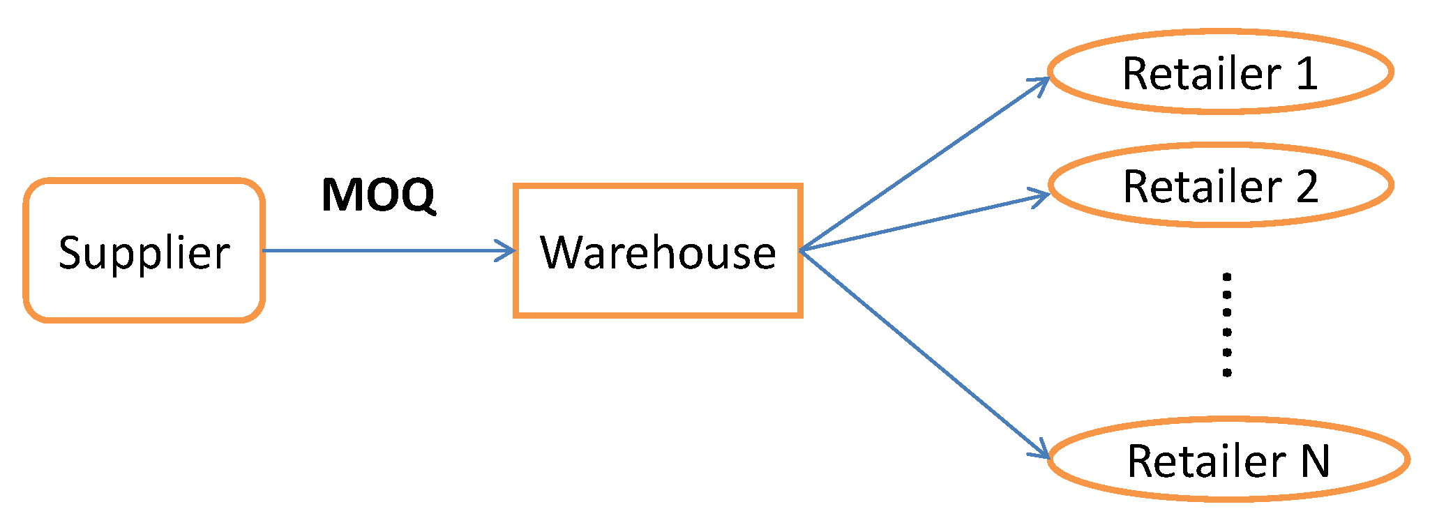
We study a two-echelon inventory system with one warehouse and multiple retailers (OWMR) in this paper. As shown in
Figure 1, the OWMR model consists of one warehouse and
N retailers. Inventory is reviewed periodically, and the horizon is infinite. In each period, retailers replenish their stocks from the warehouse, and the warehouse in turn replenishes from an external supplier. The supply chain is operated under an installation-stock based control. Linear purchasing cost is considered, but the warehouse must order either none or at least as much as a
minimum order quantity (MOQ).
The MOQ requirement is enforced by the external supplier (manufacturing facility) to achieve economies of scale, and it has been widely applied by the firms manufacturing apparel, consumer packaged goods, and chemical products. The application of a MOQ is common in practice. With the prevalence of e-commerce, MOQs have been used more and more widely, especially in online business-to-business (B2B) sourcing portals such as alibaba.com, where suppliers often impose such requirements. MOQs are also applied in manufacturing industries for products that have short lifetimes or long leadtimes. A well-known example is Sport Obermeyer, a fashion sport ski-wear manufacturer, which has a minimum production level of 600 garments in Hong Kong and 1200 garments in China per order (Zhao and Katehakis [
1]). In fact, the MOQ requirement is quite common in China and other low cost manufacturing countries, where low profit margins force manufacturers to pursue large production quantities to break even.
Retailers face independent Poisson demand processes, and they do not need to consider the MOQ requirement. Unfulfilled demands at each retailer are backlogged, incurring a backlogging cost (also called penalty cost). At the replenishment occasion of each period, the orders of all retailers are sent together to the warehouse. Orders that cannot be satisfied at the warehouse are also backlogged, but they will not incur any backlogging cost. At the end of each period, holding costs are incurred for the inventory left at both the warehouse and retailers. The objective is to minimize the long-run average system cost over an infinite horizon, achieving a sustainable inventory system. Facing such a complicated system, natural questions regard how to effectively manage this complicated inventory system: When should each installation place an order? If an order is placed, what is the optimal order quantity?
Multi-echelon inventory systems are more complex than single-echelon inventory systems. Single-echelon inventory systems only focus on the inventory position and the cost incurred at a single installation. Multi-echelon inventory systems, however, need to coordinate all installations. For example, in a serial two-echelon system, one upstream installation with a large inventory will incur a large holding cost. However, if one upstream installation does not have enough inventory, orders from the downstream installation will be delayed, and this delay may result in backlogging cost at the downstream installation. In fact, such delay at the upstream installation stands as a substantial challenge for the management of multi-echelon supply chains, and it is the biggest difference from single-echelon inventory systems.
To answer these questions, we need to first build a solid understanding of the structure of the inventory system. The OWMR model studied in this paper belongs to a pure distribution two-echelon inventory system, which is more challenging than the serial systems for the following two reasons. First, the demand process faced by the upstream installation is a superposition of the order processes of all its consecutive downstream installations. Second, in the case of shortage, the upstream installation needs to allocate current available inventory among its consecutive downstream installations, and different allocation policies will lead to different costs of the system (even with the same inventory policy and parameters).
Therefore, the allocation policy at the warehouse in the case of shortages is a key issue in the OWMR model. As suggested by Graves [
2], we assume the warehouse adopts a
virtual allocation policy, which means the orders for individual units are filled in the same order as the original demands at the retailers. Therefore, retailers’ orders are filled in the order in which they are created. This policy gives rise to a significant tractability and a near-optimal performance. With the prevalence of information science and technology, the virtual allocation policy is realistic and achievable in practice. For example, the warehouse can observe retailers’ demands in real time, and the demand information together with occurrence time are reported to the warehouse promptly.
Apart from the above, the MOQ requirement brings new challenges for the management of two-echelon inventory systems, because it reduces the inventory system’s flexibility in responding to demand, and eventually increases inventory costs. In our model, the external supplier imposes the MOQ requirement on the warehouse, whereas retailers do not need to consider the MOQ. For such a model, it is not clear how to evaluate the cost and optimize the system, and our efforts are therefore devoted to work them out.
The contributions of our paper are three-fold.
First, to the best of our knowledge, we fill a gap in the literature in the sense that we are the first to analytically study a two-echelon inventory system with a MOQ requirement over an infinite horizon. The MOQ requirement is quite common in low cost manufacturing countries. Our work enriches the literature in the areas of inventory management and MOQ requirement.
Second, we propose a new refined base stock policy for the inventory system with a MOQ requirement, and also provide optimization methods such that the optimal parameters can be easily obtained. In addition, to evaluate the system cost, we present a new position-based cost-accounting scheme, in which the cost of each unit is assigned to its first position at the warehouse.
Third, we derive tight lower and upper bounds of the inventory parameters, which not only facilitate the search for the optimal policy that minimizes the long-run average system cost, but also shed light on inventory control in reality with some useful managerial insights. Our analytical results can be referred to as a good theoretical foundation for future related research.
The remainder of this paper is organized as follows. The literature related to our paper is discussed in
Section 2. In
Section 3, the model description is presented.
Section 4 introduces a new heuristic policy developed for the inventory system with a MOQ requirement. In
Section 5, we propose a new cost-accounting scheme to evaluate the system. The optimization method of our model is discussed in
Section 6, and the paper is concluded in
Section 7.
2. Literature Review
Our paper is related with a large body of multi-echelon inventory literature that studies cost evaluation and parameter optimization. Basically, multi-echelon inventory systems include serial systems, distribution systems, assembly systems, and general networks (see [
3] for a good survey). The best-known early work for multi-echelon inventory systems may be the one by Clark and Scarf [
4], and their decomposition technique is exact for serial systems. For a classical serial system, the echelon base-stock policy is optimal for both finite horizon ([
4]) and infinite horizon ([
5]) criteria. Chen [
6] first established the optimality of
policy for a serial system with batch ordering. More recently, Shang and Zhou [
7] studied the optimal policy parameters of an echelon
policy and heuristics for a serial system with fixed costs. Since a serial system is a special case of distribution inventory systems, our work, focusing on distribution networks, can be easily extended to the serial systems. In the remainder of this section, we only review the studies on distribution systems, with a particular focus on OWMR models.
2.1. Allocation Policy at the Warehouse
A key issue in distribution inventory systems, especially in periodic-review study, is the allocation policy at the warehouse in case of shortages. Up to now, the balance assumption and the virtual allocation policy are two commonly used policies.
The balance assumption, first suggested by Clark and Scarf [
4], means that an upstream installation can make negative allocations to its downstream neighbors, or equivalently, lateral transshipment is allowed among all retailers. The balance assumption allows complete and costless reallocation of all stock in the system in every period. This implies that the warehouse stock can be used more efficiently than what is possible in reality, and therefore the balance assumption provides a lower bound for the real cost. The balance assumption has been widely applied in inventory study. Literature that uses or relies on the balance assumption includes the works in [
5,
8,
9,
10,
11,
12,
13,
14,
15,
16], and references therein.
The virtual allocation is another well-known allocation policy. It assumes that the upstream warehouse can observe the demand processes at all its downstream installations in real time. At the time when a demand event occurs, the warehouse commits or reserves a unit of its inventory (if available) to replenish the downstream installation; however, the actual shipment of this unit does not start until the shipment occasion of that period arrives. Therefore, under the virtual allocation policy, orders for individual units at warehouse are filled in the same sequence as the origin demands at the retailers, which is consistent with the first-come-first-served basis in the continuous-review model. The virtual allocation policy was first proposed by Graves [
2], and it is shown to be near optimal in many cases. After that, it was extensively used by the authors of [
17,
18,
19]. Other allocation policies include the “ship-up-to-
S” policy ([
20]), the “rationing-fraction-
” policy ([
21]), the
-policy ([
22]), the two-period allocation ([
23]), the two-interval allocation policy ([
24]), and the asymptotically optimal allocation ([
16]).
2.2. Methodologies for Distribution Inventory Systems
In general, as Simchi-Levi and Zhao [
3] summarized, there are three generic methods for distribution inventory systems: the queuing-inventory method, the leadtime demand method, and flow-unit method.
The queuing-inventory method, just as the name indicates, models the inventory systems by a queuing system. In the OWMR model, the warehouse can be interpreted as a queuing system, where the waiting customers are backorders. Most of the previous studies using queuing-inventory method consider only continuous-review systems and one-for-one replenishment. The best-known work is the METRIC (Multi-Echelon Technique for Recoverable Item Control) approximation proposed by Sherbrooke [
25]. In the OWMR model, the retailers’ leadtime may be stochastic due to possible delays at the warehouse. METRIC approximation means to replace this stochastic delay with its expectation.
The METRIC method is simple and computationally efficient because it decomposes the multi-echelon system into single-echelon systems, and therefore all the installation can be easily handed. Due to this advantage, several variations of METRIC are also proposed. Sherbrooke [
26] proposed a VARI-METRIC framework, which performs better than METRIC in a numerical study. Recently, in [
27], the authors applied the VARI-METRIC in designing an innovative model of spare parts allocation problem, aimed at minimizing backorders and ensuring system availability. Based on METRIC, Patriarca et al. [
28] developed a novel system-approach model to address the stock allocation within a complex network, where unidirectional lateral transshipment has been concretely considered. Patriarca et al. [
29] extended METRIC by considering a specific performance based contract (called PBC-METRIC), whose performance is demonstrated in a case study on a European airline that aims at reducing the ownership cost for the customer airline, while ensuring a target system performance. In [
30], the authors extended METRIC by using the zero-inflated Poisson distribution to describe the demand pattern of the high-cost spare items (called ZIP-METRIC). In an extensive case study, the ZIP-METRIC outperforms the traditional Poisson-based approach. However, due to the MOQ requirement, we cannot apply the METRIC and the extensions mentioned above in our inventory system. Specifically, the common assumption in METRIC that the (S-1, S) policy is appropriate for each item at each level (echelon), cannot hold in our system.
The leadtime demand method is similar to the classical method in single-echelon inventory systems. That is, the inventory position after ordering minus the demand during the leadtime is the inventory level (positive for on-hand inventory and negative for backorders). Given the inventory position after ordering, as long as the demand during the leadtime can be characterized, the inventory level is known and hence the cost incurred can be computed. In a continuous-review multi-echelon study, Simon [
31] used a binomial disaggregation to characterize the steady state of the inventory level for Poisson process demand. Shanker [
32] extended this work to a similar system with compound Poisson process demand. Graves [
33] proposeed a two-moment approximation for the steady-state distribution and showed that this approximation has a better performance than METRIC in a numerical study.
The flow-unit method keeps track of each supply unit as it moves through the system. Our work also use this method. Specifically, it characterizes the time between the placement of an order and the occurrence of its assigned demand unit. If this time is longer than the leadtime, backlogging cost is incurred; otherwise, holding cost is incurred. Axsäter [
34] first used this method to evaluate the cost of a continuous-review inventory system with one-for-one replenishment policy and independent Poisson demand. Later on, Axsäter [
35] extended this work to systems with batch ordering. Many extensions have been studied, for example, the installation or echelon stock
policies with Poisson or compound Poisson demand processes, as proposed in [
36,
37,
38].
Our work also shares a common theme with the cost-accounting work. Levi et al. [
39] proposed a new marginal cost accounting scheme for a single-echelon inventory system. We both focus on costs incurred by the units that ordered in the same period. However, in their scheme, they focused on the backlogging cost incurred by these units for a single period due to non-stationary inventory parameters (see [
40] for capacitated models and [
41] for serial systems). However, we focus on the duration of a state (in stock or not) of one unit in the inventory system. In addition, we consider a pure distribution network with a MOQ requirement. Therefore, our work is fundamentally different from theirs.
2.3. MOQ Requirement
In the area of MOQ, Fisher and Raman [
42] first considered a two-period model with a MOQ requirement in each period. They worked out the optimal order quantity by using stochastic programming methods. Zhao and Katehakis [
1] introduced the concept of M-increasing function and first partially characterized the optimal policy for multi-period inventory systems with MOQ. For the uncharacterized part, the authors gave easily computable upper bounds and asymptotic lower bounds for these intervals. However, for the characterized part, the optimal policy is complicatedly structured and difficult to implement in practice. Zhou et al. [
43] proposed a two-parameter heuristic policy for a single-echelon inventory system with a MOQ requirement and demonstrated that the performance of this policy is close to the optimal policy, except for a few cases when the coefficient of the demand distribution is very small. For the same model, Kiesmüller et al. [
44] proposed a modified base-stock policy, which is a special case of the policy proposed by Zhou et al. [
43]. In the numerical study, the authors showed that this policy has a good performance in most cases. This modified base-stock policy has only one parameter and is easy to implement. Zhu et al. [
45] studied a single-item periodic-review stochastic inventory system with both minimum order quantity (MOQ) and batch ordering requirements.
The most closely related papers to our work are those in [
17,
18]. Axsäter [
17] studied a OWMR model with Poisson demand where each facility applies a periodic-reviewed order-up-to-S policy, and then Forsberg [
18] extended this work to a OWMR model with compound Poisson demand. Both groups used the flow-unit method to study a OWMR model where the warehouse is assumed to adopt a virtual allocation policy. The major difference between our paper and the above two is that we assume the warehouse faces a MOQ requirement and thus adopts a different inventory policy (different from their order-up-to-S policies). Note that the MOQ requirement brings new challenge to keep track of a single unit, whereas in [
17,
18], the warehouse does not need to consider MOQ and each ordered unit from the retailers will trigger a virtual replenishment of the warehouse.
Finally, in addition to the above three streams of literature, our work is also related to papers on the uncertainty management in supply chains and on the use of classic models. For example, Fera et al. [
46] defined a system dynamics model to assess competitiveness coming from the positioning of the order in different supply chain locations. Miranda et al. [
47] showed the improvements of an alternative approach for the calculation of the multi-item economic order quantity in presence of space constraints. Fera et al. [
48] presented an algorithm that helps the aggregator of energy loads in carrying out its daily decisions, using an economic objective function.
3. Model Description
We consider one warehouse (Installation 0) and
N retailers (Installations 1, 2, ⋯,
N), as shown in
Figure 1. Retailers face independent Poisson demand processes. Unfulfilled demands at each retailer are backlogged. Retailers replenish their stocks from the warehouse, and in turn the warehouse replenishes from an external supplier. The lead time is assumed to be
periods between the warehouse and retailer
i, and
periods between the external supplier and the warehouse. Orders that cannot be immediately satisfied at the warehouse are also backlogged. There are linear holding costs at both the warehouse and all retailers, while the backlogging costs are only incurred at retailers. We also assume the warehouse and retailers select units to satisfy the demands based on a first-ordered-first-consumed rule, and hence they select the oldest units in stock to satisfy the most recent demands. For example, the units ordered by the warehouse in period
n can be used to satisfy retailers’ demand only when all the units ordered by the warehouse in period
are used out.
Notably, there is a MOQ requirement for the warehouse. It restricts that the warehouse, if it orders, must order at least M units, where M is a specified minimum order quantity. No such enforcement is imposed on retails, and each retailer is allowed to order any quantity. The supply chain is operated under installation-stock based control. We assume that each retailer i adopts a base-stock policy with the order-up-to level . The warehouse, due to the MOQ requirement, adopts a refined base-stock policy with reorder point (which is discussed below). Since each retailer adopts a base-stock policy, we assume that each demand unit at the retailer will trigger a virtual order to the warehouse and the warehouse allocates its inventory based on the virtual allocation policy.
Our objective is to minimize the long-run average system cost, including the ordering, holding, and backlogging cost, over an infinite horizon. Note that we set the ordering cost to be zero because linear ordering cost can be ignored under the average cost criterion (see, e.g., [
49]). In addition, note that
M,
, and
(
) are all integers.
The
sequence of the events operate as follows. (1) The warehouse orders and then the periodic delivery from the external supplier arrives. (2) Retailers place orders to request replenishment from the warehouse. (3) The periodic delivery from the warehouse arrives at each retailer. (4) The stochastic demand takes place at all retailers. Inventory and backorders are assessed and then costs are charged. The primary notations used in the paper are summarized in
Table 1.
4. A Refined Base-Stock Policy for MOQ
In this section, we focus on a single-echelon stochastic inventory system with a MOQ requirement. Kiesmüller et al. [
44] proposed a generalized one-parameter base-stock policy (referred as
S policy) that considers the MOQ requirement. Their policy works as follows: no order is placed when the inventory position is not less than the level
S; otherwise, an order is placed to raise the inventory to
S. However, if this order is smaller than the MOQ (i.e.,
M), the order quantity is increased to
M. Let
be the inventory position before ordering in period
n, and then the order quantity in period
,
, can be described as
We can see that the principle of the above
S policy is to raise the inventory position to the level
S as long as the inventory position is below
S. If the difference between the current level and the aimed level (
S) is less than
M, then the order quantity is raised to
M due to the MOQ requirement. Therefore, this policy is a generalized base-stock policy with the base-stock level
S. In a numerical test, Kiesmüller et al. [
44] showed this policy has near-optimal performance in most cases.
However, there is one implicit drawback of the S policy. Suppose that the unit holding cost is quite large, then the firm has no incentive to hold much inventory, and S can be negative. Assume (we show that the optimal S cannot be less than below), in the case that the inventory position before ordering is less than , to raise the inventory position to S, the order quantity should be according to the S policy. However, if S is negative, even if the inventory position is raised to S, it will still incur backlogging cost. Obviously, compared to this, raising the inventory position to zero is a better alternative. The same problem exists when the inventory position is less than S and higher than . The firm has no incentive to keep the backlogging state in such cases and should try to raise the inventory position to zero at least.
Therefore, to tackle the above drawback, we propose a refined base-stock policy, which works as follows: if the inventory level is less than the level
S, an order is placed to raise the inventory position to the maximum between
S and zero (if this order is smaller than
M, the order quantity is increased to
M); otherwise, no order is placed. Formally, the order quantity
is defined by
In our policy, if the inventory level is less than S, we place an order to keep the inventory position non-negative. However, in the S policy, it is possible that the inventory is still in the backlogging state after ordering. This is the major difference between our policy and the S policy.
Analysis Based on Markov Chain
Particularly, our policy is reduced to the
S policy if
. In such case, we can use the same method to analyze the system as Kiesmüller et al. [
44]. Considering this, in the remainder of this section, we deal with the case where
.
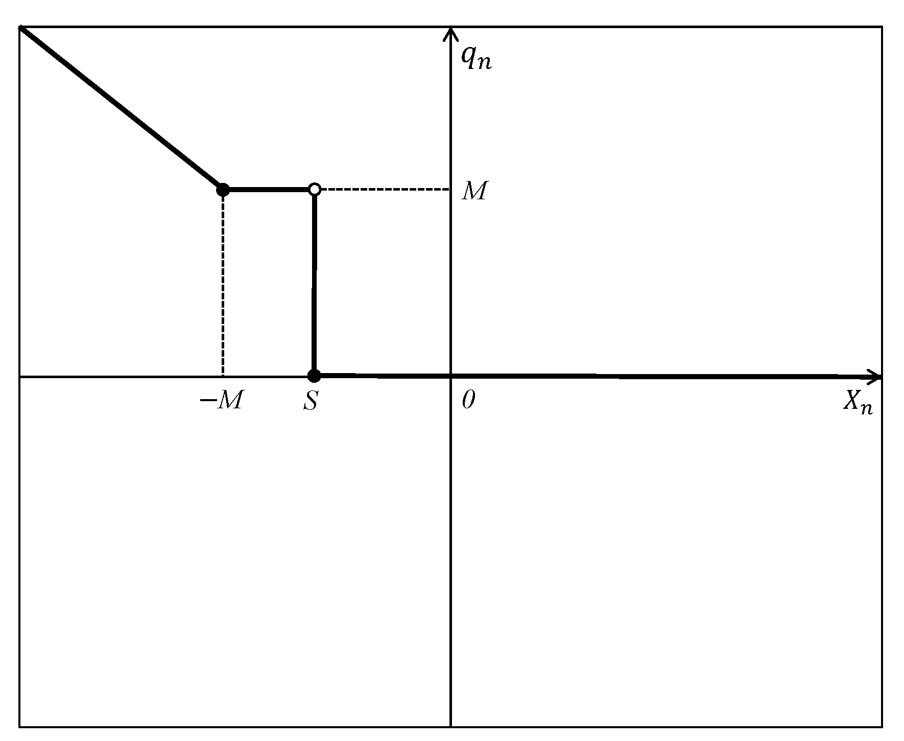
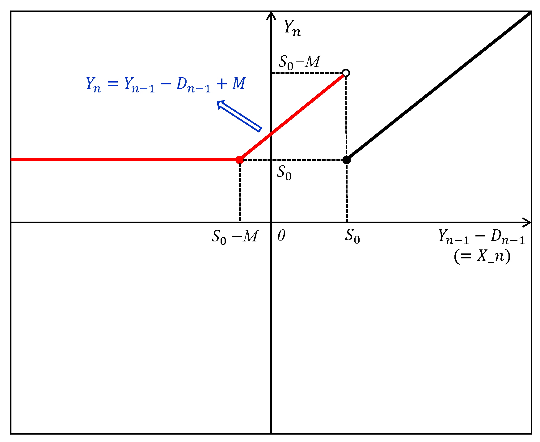
Given
and inventory position
, the order quantity
can be rewritten as (see
Figure 2 for illustration)
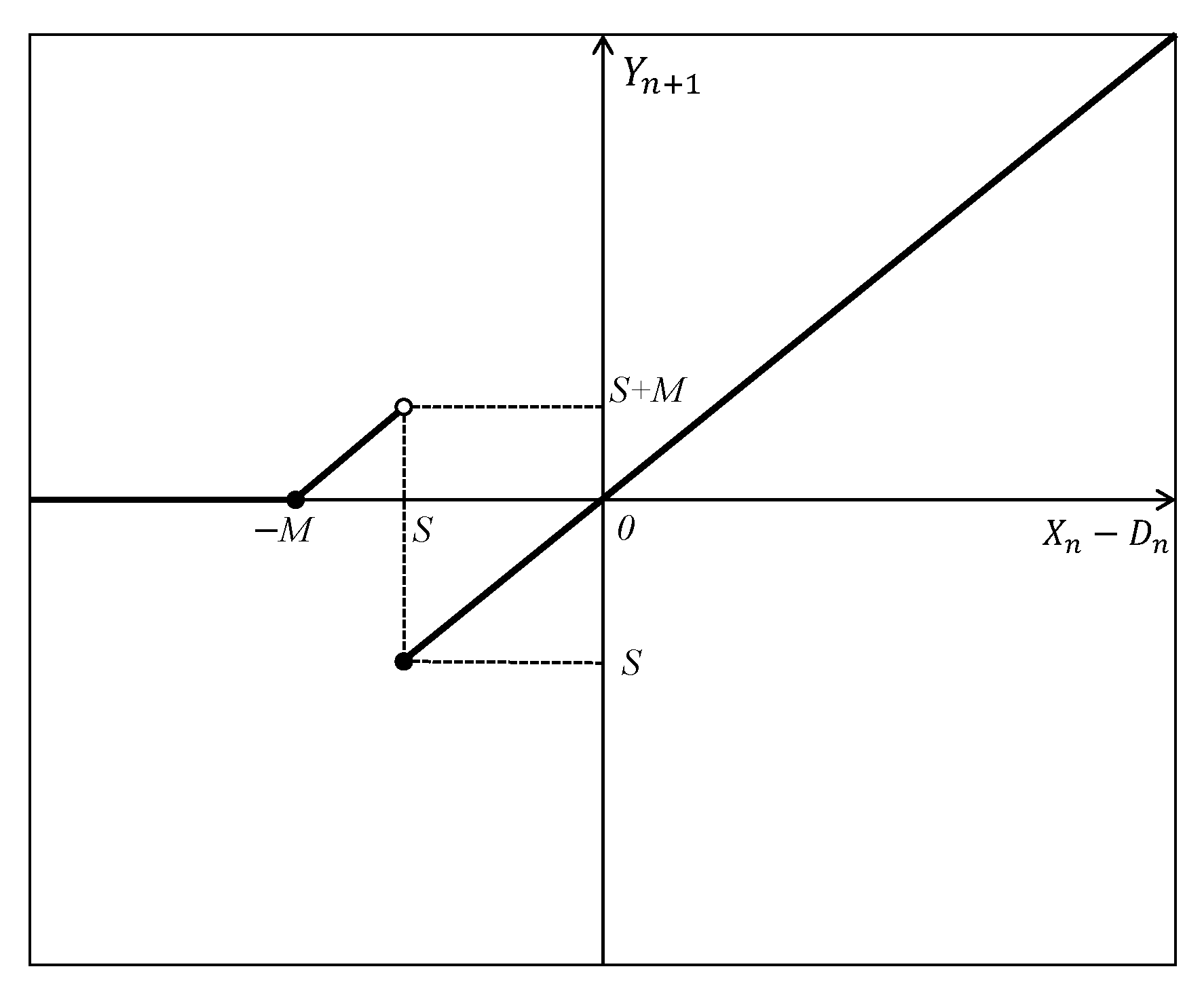
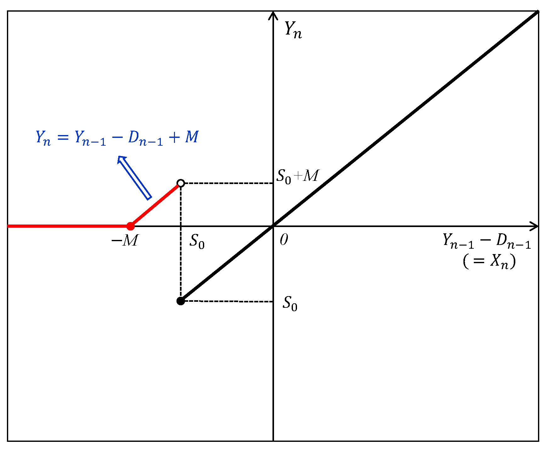
Let
be the inventory position after ordering in period
n. The inventory balance equation follows from (see
Figure 3 for illustration)
where
is the demand in period
n.
It is clear that
is a Markov chain with a finite state space
, i.e.,
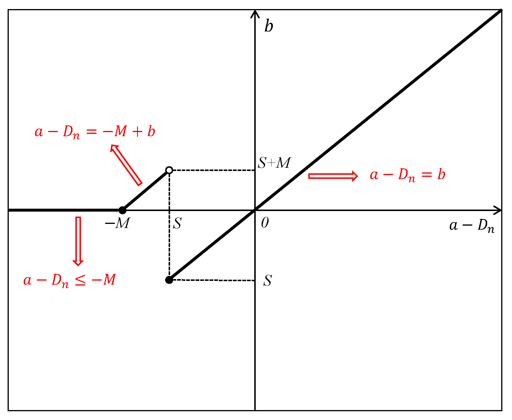
. Then, the transition probabilities
can be derived as (see
Figure 4 for illustration)
where
equals to
if
, and zero otherwise.
For the state space
, we define state
i as the integer
, where
. Since the above Markov chain is irreducible and positive recurrent, the unique steady state probabilities
exist, where
denotes the long-run average proportion of time in which the inventory position
y is
. Moreover, since the Markov chain is aperiodic,
is the limiting probability that the chain is in state
i. Let
; in the steady state, we have
Therefore, we can compute the stationary probabilities by solving the above linear Equation (
1).
Now, we can compute the long-run average cost
for a single installation:
where
is the single-period inventory cost for a single installation when the inventory position is at
, and can be expressed as
where
h is the unit holding cost and
p is the unit backlogging cost. Let
be a minimizer of
. It is easy to see that
is convex and
as
. Then,
is convex because it is a summation of several convex functions. Let
be the optimal
S that minimizes
. The following proposition provides lower and upper bounds for
.
Proposition 1. satisfies .
Proof of Proposition 1. Based on the definitions of
and
, we prove the proposition by contradiction. First, assume
. As
is non-decreasing when
, we have
,
. It implies
This contradicts the definition of , and hence .
Second, assume
. Since
is non-increasing when
, we get
,
. It implies
This also contradicts the definition of
. Therefore, we arrive at
Moreover, can be derived from . □
Proposition 1 helps us to search the optimal level . The intuition of this proposition is to keep in the set of integers , i.e., . Recall that is the state space for the inventory position after ordering. If one S cannot guarantee that falls in this set, then this S cannot be the optimal one. Proposition 1 provides a lower bound and an upper bound for . Obviously, , which validates our previous statement that .
To conclude this section, we propose a refined base-stock policy for the stochastic inventory system with a MOQ requirement. In the remainder of this paper, we assume the warehouse in our OWMR model adopts this policy to control its inventory with .
5. A Position-Based Cost-Accounting Scheme
We introduce a new cost-accounting scheme and use this scheme to evaluate the cost of our model in this section. We first focus on the inventory position of the warehouse. Note that the warehouse faces a superposition of the order processes of all retailers. Since each retailer applies a base-stock policy, each demand unit at retailers will trigger a virtual order to the warehouse. Due to the superposition property of Poisson process, the warehouse faces a Poisson demand process with arrival rate
. Then, we can characterize the
inventory position of the warehouse as in the single-echelon system studied in
Section 4. We next suppose that, in the steady state, the distribution of the warehouse inventory position
is known (see Equation (
1)). With a little abuse of notation, we use
to denote the steady-state probability that the warehouse inventory position is
y.
We compute the costs associated with the units ordered by the warehouse in the current period (in which the ordering happens), that is: (1) if no order is placed at the warehouse, then no cost is incurred in that period; and (2) if some units are order by the warehouse in one period, we compute all the costs associated with these units. Note that, in the latter case, the costs associated with these units may incur in other periods, e.g., holding costs incurred in the future periods; however, under our framework, we assign all these costs to the current period.
In each period, if the warehouse places an order, each ordered unit will have a corresponding position at the warehouse for that period. For each position at the warehouse, there will be a corresponding expected system cost C, which is the total cost associated with the unit at this position, including holding cost at the warehouse, holding and backlogging cost at retailers. As long as one unit is ordered by the warehouse, it will have a position at the warehouse and its expected overall cost through the system is determined. In other words, for a unit with position , its overall cost depends on the position . Therefore, our cost-accounting scheme is a position-based framework.
The long-run average cost
can be characterized as
where
is the expected cost incurred by the unit with position
when it is ordered by the warehouse. Since
,
, and
, both
and
are possible.
Remark 1. The position of a unit (before it is used to satisfy retailer demands) at the warehouse will decrease as the number of ordered units increases. In our position-based scheme, we only focus on the position of a unit in the period when this unit is ordered by the warehouse. Therefore, hereinafter, we use “a unit with position ” to denote the unit whose position is in the specific period when it is order by the warehouse.
Remark 2. In Equation (
2)
, is the probability that inventory position after placing an order equals to y. This probability is less than the steady state probability discussed earlier, and we can easily verify it from . We do not consider the case , because no cost is incurred if no ordering. In the sequel, we first discuss how to compute the cost function , and then derive the inventory position probability .
5.1. Computation of Cost Function
For an arbitrary unit (hereinafter referred as unit
w) with position
when it is ordered by the warehouse, the cost function
is formulated as
where
is the expected warehouse holding cost incurred by unit
w, and
is the expected backlogging and holding cost incurred by unit
w at retailer
i. Because the warehouse faces a Poisson process demand and adopts the virtual allocation policy, this unit is assigned to retailer
i with probability
.
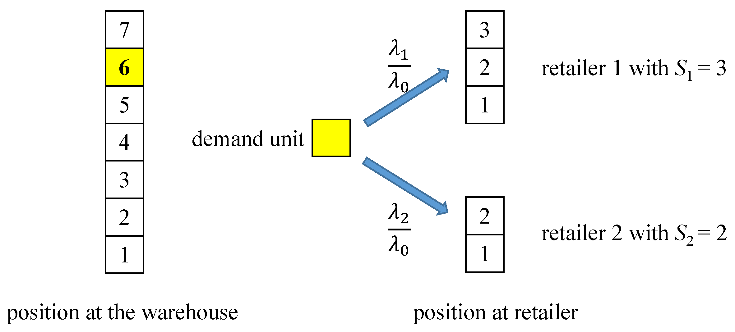
Figure 5 shows an example of our position-based cost function, where there are a demand unit of position
at the warehouse, and two retailers, one with order-up-to level
and the other with
. Therefore, the expected holding cost at the warehouse is
, and the expected backlogging and holding costs at Retailers 1 and 2 are
and
, respectively. The total cost is
.
We extend the notations to be used in this section in
Table 2.
5.1.1. Computation of .
Suppose that unit w is ordered by warehouse in period n. Since the lead time is periods, this unit arrives at the warehouse in period . Recall that is the time difference between the period when unit w is ordered by the warehouse and the period when unit w is ordered by a retailer. If , the unit first arrives at the warehouse, and then is requested by a retailer after some periods. Therefore, the number of periods with holding cost is . If , the unit has not reached the warehouse when it is ordered by a retailer, and there will be no holding cost.
Consequently, for a single unit with position
, the expected holding cost incurred at the warehouse,
, can be expressed as
where
gives the distribution of
that is dependent on
.
In the following, our effort is devoted to determine the distribution of . The position is determined at the moment unit w is ordered by the warehouse, therefore, unit w will be used to satisfy the th warehouse demand after it is ordered by the warehouse. As mentioned earlier, both and are possible.
For a given
, the distribution of
can be characterized by
where
represents the total demand at the warehouse over
periods,
and
We next study the distribution of if , followed by two cases. The first case is and , which means unit w is used to satisfy the retailer’s order in the last period. This implies that unit w is requested by one retailer in the last period, and thus .
The second case is
and
. Since
, unit
w is used to satisfy the retailer’s order earlier, implying that unit
w is requested by one retailer in one of the earlier periods, and thus
can take the values from
. Specifically, if
, unit
w is requested by one retailer one period before it is ordered by the warehouse. Hence, in the period when unit
w is requested by one retailer, the inventory position of the warehouse at the end of that period is less than
, and this will trigger one order including unit
w from the warehouse to the supplier. Therefore, for any unit
w with a position
, it must have
, i.e.,
which means this unit is used to satisfy the demand in the last period.
We are left to analyze the position
. The probability of
is
If
, unit
w is requested two periods earlier before it is ordered by the warehouse. To compute the probability of
, we need to condition on the inventory position one period earlier. Suppose unit
w is ordered by the warehouse in period
n,
implies it is requested by one retailer in period
. This means that the inventory position at the end of period
is not less than
, while the inventory position at the end of period
must be less than
. Following the same logic, we can get the probability of
as follows
where
.
To conclude, for a single unit with position
, based on the values of
, the detailed probabilities
are given in Equations (
4)–(
7), and the computation in Equation (
3) of
is completed.
5.1.2. Computation of .
We are left to compute the cost for a single unit incurred at retailer
i,
. Let
denote the possible delay at the warehouse when unit
w is ordered by a retailer. Note that
means the unit will be shipped to the retailer after
periods it is ordered by the retailer. If
, the unit has already been at retailer
i for
periods when it is ordered by customer demand. In this case, it will incur a holding cost
. If
, the unit is still on the way to retailer
i and will arrive after
periods, then it will incur backlogging cost
. Consequently, the cost incurred by this unit at retailer
i,
, is computed by
where
gives the distribution of
that is dependent on
, and
gives the distribution of
that is dependent on both
and
.
We first derive the probability . Since , we get
- (1)
- (2)
if
and
,
- (3)
Next, we work on the probability . At the retailer level, after placing an order to the warehouse, the inventory position of retailer i reaches its base stock , as do the other retailers (according to the base-stock policy). Note that the inventory position of retailer i here includes the units that may have not reached the warehouse but have already been assigned to retailer i.
At the warehouse level, for a unit
w with position
, suppose it is ordered by the warehouse in period
, and is ordered by retailer
i in period
n. That is, the time difference between the two periods is
. The total demand over these
periods is
. Hence, in period
, there are also
units ordered by the warehouse after unit
w. For any unit among them, if it is assigned to retailer
i, it will have a higher position at retailer
i than unit
w. This is because unit
w is virtually ordered earlier than these units by retailer
i. Let
, and we decompose these
units and explore how many will “be above” (have a higher position at retailer
i if is assigned to retailer
i) unit
w. Let
denote the numbers of such units. Obviously,
. The unit
w has a position of
at retailer
i in period
, and thus it will be used to satisfy the
th demand starting from period
. At the warehouse level, when a new demand unit arrives, it is previously ordered from retailer
i with a probability
. Consequently, given that
takes the value of
, the conditional probability that
units (out of these
units) are ordered from retailer
i, can be determined as
Remark 3. In [31], a similar binomial distribution is proposed to disaggregate the backorders. In our method, we disaggregate all the demand units after unit w by Equation (
9)
; however, Simon [31] disaggregated only the possible backorders of one period. Now, for the unit
w with position
at the warehouse, we have
where
denotes the demand over
periods (i.e., from period
n to period
) and
denotes the demand in period
. Then, we can compute the joint distribution of
and
by using Equations (
9) and (
10) as follows
Since the position at retailer
i is
, from Equation (
11), we can know the joint distribution of
and
as
The distribution for
then is defined by
Similar to the process at the warehouse level, if
, we can derive the following distribution of
where
and
If
, the unit is ordered in the last period; therefore,
and we have
This is similar to the case and where at the warehouse.
Remark 4. Equation (
13)
implies that the distribution of depends on , whose distribution depends on from Equation (
12)
. This means that the distribution of also depends on . To conclude, the probability
can be computed based on Equations (
12)–(
14). Up to now, given the position at the warehouse
, we can compute the cost associated with unit
w by Equations (
3) and (
8). We next provide the derivation of the distribution of the inventory position
.
5.2. Computation of Inventory Position Probability
We extend the notations to be used in this section in
Table 3. Please note that
represents the inventory positions at the warehouse, which is updated immediately after ordering.
In period
n, given an inventory position
after an ordering
, we need to compute the inventory position probability
. We choose to conditioning on the inventory position in period
, i.e.,
. For any
, we have
For the conditional probability, depending on the value of , we have two cases:
Figure 6 and
Figure 7 plot the relationships between
and
with
and
, respectively. In both figures, the red bold lines represent the
after an ordering
, and the black bold lines represent a zero ordering, i.e.,
.
Next, we discuss how to derive the distribution of the position of an arbitrary unit w at the warehouse, since it is a prerequisite in the computation of cost function . Similar to the above, we have two cases to follow: the first case is , and the second case is .
Case 1: . Based on Equations (
15) and (
16),
takes values from
. If
, then
and
(see
Figure 6). This implies that, in period
n, the warehouse orders
M units in period
n. The unit
w is uniformly distributed in these units, and therefore
where
represents a Uniform distribution in the interval
, and
, i.e., the starting position.
If
, then
can be larger than
M. Unit
w is still uniformly distributed in these
units. To obtain the distribution of
, we must know the distribution of
. We next characterize the distribution of
for
. Since
, we have
(see
Figure 6), and the distribution of
is defined by
The order quantity is
in period
n. The unit
w is uniformly distributed in these
units, hence we have
We should note that the distribution of depends only on and is independent of .
Case 2: . Based on Equations (
15) and (
17),
takes values from
. If
, then
and
(see
Figure 7). Similar to the previous analysis, we have
If
, then
can be larger than
M. We have
(see
Figure 7), and the distribution of
is defined by
Similar to the previous analysis, the distribution of
is
Remark 5. Our position-based cost-accounting scheme uses flow-unit method to evaluate the cost of the whole system. Levi et al. [39] used a similar idea of holding cost accounting; however, due to their non-stationary parameter setting, they evaluated the backlogging cost for a single period, not for a single unit in our scheme. Axsäter [34] used a flow-unit to evaluate the cost of a continuous-review model without the MOQ requirement. A distinct feature of our work is to assign the cost of a single unit to its position at the warehouse, and we characterize the distribution of this position. 6. Optimization
We have shown how to evaluate the cost of our model with given inventory parameters . In this section, we discuss how to optimize our model and find the optimal parameter that minimize the long-run average cost.
We first note that depends only on , which in turn depends only on , and is dependent on . This implies that, for a given , we can optimize each retailer i separately with respect to . Let denote the optimal value of for a given .
Proposition 2. For a given , is convex in each .
Proof of Proposition 2. denotes the long-run average system cost, which consists of the cost incurred at the warehouse and the costs incurred at all retailers. For a given
, the cost incurred at the warehouse is independent of
. We next only consider the cost incurred at retailer
i. If this cost is convex in
, then we can have the total cost
L is convex in
, recalling that we can optimize each retailer
i separately with respect to
. For a given
, the distribution of backlogging quantity can be determined, and we can decompose these backlogging units using the same way as Equation (
9). Given the distribution of backlogging quantity for retailer
i, we can know the distribution of delay time at the warehouse caused by these backlogging units. With a little abuse of notation, we use
to denote the delay time at the warehouse for retailer
i. Now, for a given
, we know the retailer’s leadtime
and the distribution of its delay time
. To optimize retailer
i,
can be seen as an additional leadtime, and then the problem is reduced to a single-echelon retailer
i with a leadtime
. For each possible value of
, the cost incurred at retailer
i is a convex function of
, which can be easily obtained from the typical Newsvendor problem with a base-stock policy. Taking the expectation with respect to
, we can conclude that the expected cost is convex in
and so is the total cost
L. □
Proposition 2 implies that when other parameters are fixed, for each specific retailer, there exists a unique order up to level such that the total inventory cost
is minimized. This result is consistent with that in continuous-review model without MOQ requirement (see, e.g., [
34]). Using Proposition 2, we can find the corresponding
for each
. We next try to find some bounds for
and
.
Proposition 3 (Lower bound). and for each .
Proof of Proposition 3. Since is straightforward by Proposition 1, we only need to prove for each . We prove this by contradiction. Suppose there exist an optimal for an arbitrary retailer . Then, compare this system to another system with the same parameters except for . We can easily find that the cost incurred at the warehouse and retailer are all the same in the two different systems. The only difference is the cost incurred at retailer i. For retailer i, means it always has backlogging units in every period and the expected cost is . Note that there is no holding cost in each period if . Similarly, if , the expected cost is and there is also no holding cost. Obviously, the system with has a better perform than the system with . This contradicts the optimality of . Therefore, we have . □
Intuitively, the installations have no incentive to keep the inventory position always below zero. More specifically, it can never be optimal for a warehouse to keep the inventory too low () or for a retailer to hold negative inventory (). Proposition 3 provides a lower bound for and . A loose upper bound for is such that , where is the probability that takes a value smaller than for and is a tiny value that is close to zero. In others words, if , the possibility that there is a delay at the warehouse is small enough. This implies that backlogging at the warehouse seldom occurs.
Now, we have the lower bound and upper bound for , and for each possible integer in the interval, we can search the corresponding optimal . Therefore, we can find the globally optimal parameters .
We next work to derive tight bounds for the inventory parameters. First, we have the following lemma.
Lemma 1. , .
Proof of Lemma 1. For a given , the problem of determining the inventory parameter at retailer i is reduced to the classical Newsvendor problem whose leadtime is stochastic due to the possible delay at the warehouse. Furthermore, if we consider the distribution of the random delay encountered at the warehouse, obviously, the cumulative distribution function for is stochastically larger than that for . Therefore, the optimal inventory order-up-to level for is not less than that for . □
Lemma 1 implies that when the warehouse holds more inventory, the optimal order-up-to level of a retailer tends to decrease. The intuition is that, when the warehouse holds more inventory, the inventory shortage at the warehouse is less likely to happen, or, in other words, it is more likely for the warehouse to satisfy a retailer’s order, and thus the retailers tends to hold less inventory.
Define
where
is the inverse cumulative demand distribution functions of retailer
i over
periods. Obviously,
is the optimal inventory parameters for retailer
i in a single-echelon model with leadtime
periods. In other words,
is the optimal
when there is no delay at the warehouse. Then, we have the following proposition.
Proposition 4 (Lower bound)
. is the lower bound for , i.e., , where is given in Equation (
18)
. Proof of Proposition 4. Recall that
. By induction, we have
where
is the optimal
when
goes to infinity. When
is sufficiently large, we know that there is no delay at the warehouse, and the optimal
is
by definition, i.e.,
. □
The intuition of Proposition 4 is straightforward. If the warehouse has enough inventory, retailers have no incentive to keep much inventory; on the contrary, if there is a long delay at the warehouse, retailers have much incentive to keep more inventory to avoid possible shortages. The biggest difference of retailer i in our model from that in the single-echelon model is that retailer faces possible delay at the warehouse in case of shortages. This delay can be as long as periods, and as short as 0 period. Then, retailer i can be treated as a single-echelon retailer with leadtime periods (). Therefore, is a lower bound for .
Remark 6. In [34], there is also an upper bound for , however, their upper bound does not hold in our problem. This is because, in [34], the maximum possible delay at the warehouse is periods, while in our problem the maximum delay can be longer than periods due to the existence of MOQ constraint. We next provide a more tight upper bound for .
Proposition 5 (Upper bound). is the upper bound for , i.e., , where is obtained by minimizing over the set .
Proof of Proposition 5. We know that and . For , the corresponding optimal is due to Lemma 1 and Proposition 4. By the definition of , we can have for such . Therefore, the optimal must satisfy . □
Recall that
, thus
must satisfy
Moreover, we know that, for each given , is convex in each , and . Clearly, to obtain the optimal inventory parameters, we only need to enumerate , and the corresponding .
7. Conclusions
A two-echelon inventory system with a MOQ requirement is analytically studied in this paper, where there are one warehouse and multiple retailers. In each period, retailers replenish their stocks from the warehouse, and the warehouse in turn replenishes from an external supplier, but the warehouse must order either none or a quantity no less than MOQ. The MOQ requirement is quite common in China and other low cost manufacturing countries, where low profit margins force manufacturers to pursue large production quantities to break even and achieve economies of scale. For the retailers, we assume they adopt the base stock policy. However, for the warehouse, due to the MOQ requirement, we propose a new heuristic ordering policy, called refined base stock policy, which particularly considers the case of negative base stock S.
Our objective is to minimize the long-run average system cost over an infinite horizon. To this end, we present a position-based cost-accounting scheme to exactly evaluate the system cost. Specifically, once the warehouse places an order, each ordered unit will have a corresponding position at the warehouse; and for each of such positions, we associate it with a corresponding expected system cost, including holding cost at the warehouse, and holding and backlogging cost at retailers. Built upon this position-based scheme, we derive lower bound and upper bound for the inventory parameters, which facilitate the search of optimal policy. In addition, by optimizing the system, we can also derive some managerial insights. For example, when the warehouse holds more inventory, the optimal order-up-to level of a retailer tends to decrease.


