Bi-Objective Scheduling Optimization for Discrete Time/Cost Trade-Off in Projects

Abstract

In sustainable project management, time and cost are two critical factors affecting the success of a project. Time/cost trade-offs in projects accelerate the execution of some activities by increasing the amount of non-renewable resources committed to them and therefore shorten the project duration. The discrete time/cost trade-off problem (DTCTP) has been extensively studied during the past 20 years. However, due to its complexity, the DTCTP—especially the DTCTP curve problem (DTCTP-C)—has only been solved for relatively small instances. To the best of our knowledge, there is no computational performance analysis for solving the DTCTP-C on large project instances with up to 500 activities. This paper aims to fill this gap. We present two bi-objective heuristic algorithms for the DTCTP-C where both project duration and cost are minimized. The objective is to obtain a good appropriate efficient set for the large-scale instances. The first algorithm is based on the non-dominated sorting genetic algorithm II (NSGA-II) and uses a specially designed critical path-based crossover operator. The second algorithm is a steepest descent heuristic which generates efficient solutions by iteratively solving the DTCTP with different deadlines. Computational experiments are conducted to validate the proposed algorithms on a large set of randomly generated problem instances.

1. Introduction

The importance of time/cost trade-offs in projects have been recognized since the development of the critical path method (CPM) in the late 1950s [1]. Sustainable project management requires the resources to be used in an economical and sustainable way [2,3,4]. In project management, it is desirable that shorter project duration is achieved at a lower total cost. The project duration can usually be shortened by accelerating the execution of activities. Most often expediting the activity durations needs to allocate more resources to these activities. In many real-life cases, such as construction projects, the resources (e.g., human resources or heavy equipment) tend to be discrete and measured by a single non-renewable one (capital or cost). Therefore, the duration of project activities can be treated as discrete non-increasing functions of the cost. This results in the discrete time/cost trade-off problem (DTCTP) [1]. Harvey and Patterson [5] and Hindelang and Muth [6] first proposed the DTCTP, which is a special case of the multi-mode resource-constrained project scheduling problem [7].

In the DTCTP, each activity has multiple execution modes which are characterized by specific time and cost combinations. In terms of the objective function, the DTCTP can be divided into three versions: the deadline problem (DTCTP-D), the budget problem (DTCTP-B) and the time/cost trade-off curve problem (DTCTP-C). In the DTCTP-D, given a set of modes and a project deadline, the objective is to minimize the total project cost by specifying an execution mode for each activity. In the DTCTP-B, a project budget is given and the objective is to determine the modes that minimize the project makespan. In the DTCTP-C, the objective is to determine the Pareto curve that minimizes the project makespan and cost simultaneously. In the remainder of this paper, we focus on the DTCTP-C.

Numerous exact and heuristic methods have been proposed for solving the DTCTP. Because the DTCTP is strongly NP-hard [8], exact algorithms—such as a branch and bound procedure and dynamic programming—can only solve relatively small instances [9,10,11,12]. Heuristic or meta-heuristic methods are more practical for solving large instances within a reasonable time [13,14,15]. For more detailed excellent literature reviews on the DTCTP, we refer to De et al. [9] and Demeulemeester and Herroelen [1].

Despite the vast majority of the research efforts in the DTCTP, there are few studies that have considered solving the DTCTP with more than 200 activities. Sonmez and Bettemir [16] developed a hybrid genetic algorithm for the DTCTP-D and tested it on problem instances with up to 630 activities. However, they only use ten instances to evaluate their algorithm which limits the generalizability of the algorithm. To the best of our knowledge, there are no heuristic algorithms for the DTCTP-C that solves representative instances with up to 500 activities in the existing literature. However, in practice, it is common that a project will most likely consist of hundreds of activities [17]. This motivates us to study efficient heuristic algorithms. Moreover, the lack of computational performance analysis is another common drawback for the past research in the DTCTP. Some papers only used simple examples to test their algorithms [18,19], which usually cannot fully prove the effectiveness and adaptability of the algorithms.

The purpose of this paper is to develop and verify two heuristics and to obtain a good appropriate efficient set for the large-scale DTCTP-C. The contributions of this paper are three-fold:

(1)

We propose a bi-objective hybrid genetic algorithm (BHGA) for the DTCTP-C by introducing a critical path based crossover operator in the non-dominated sorting genetic algorithm II (NSGA-II) [20]. As an effective multi-objective optimization meta-heuristic algorithm, NSGA-II has been widely used to solve the DTCTP [21,22]. Our BHGA further exploits the knowledge of the DTCTP-C and enhances the searching efficiency of the NSGA-II for the DTCTP-C.

(2)

We propose a steepest descent heuristic for the DTCTP-C to obtain efficient solutions by iteratively solving the DTCTP with different deadlines. We design a special neighborhood search procedure based on the inherent characteristics of the DTCTP-C. Our experimental results show that the proposed steepest descent heuristic outperforms the NSGA-II based BHGA.

(3)

We conduct extensive computational performance analysis for the proposed heuristics. We use factorial experimental design to randomly generate a large number of instances (with up to 500 activities) in order to validate and compare our heuristic approaches.

This paper is organized as follows. In the next section, we give the description and the model formulation of the DTCTP-C. Section 3 provides a bi-objective hybrid genetic algorithm for the DTCTP-C. In Section 4, we propose a steepest descent heuristic for the DTCTP-C. In Section 5, we present the computational results. Finally, Section 6 concludes the paper with future research directions.

2. Problem Statement and Model Formulation

2.1. DTCTP-C

The DTCTP-C under study is described as follows. A project network G = (N, A) is represented in activity-on-node format, where the set of nodes N denotes the activities $N=\left\{1,\dots ,n\right\}$, and the set of directed arcs A represents the finish–start, zero-lag precedence relations $A\subseteq N\times N$. The nodes are topologically numbered from the single start node 1 to the single terminal node n, n = |N|, where nodes 1 and n are dummy activities. Each activity i (i = 1, …, n) has |M_i| modes, characterized by a duration–cost pair (d_ij, c_ij), j = 1,…, |M_i|, where $M_i$ is the set of modes of activity i, $M_i=\left\{1,2,\dots ,m\right\}$. The duration d_ij of an activity $i\in N$ is a discrete, non-increasing function of the amount of a single non-renewable resources (c_ij) committed to it, i.e., if k < l (k, l $\in$ M_i), then d_ik < d_il and c_ik > c_il. The dummy activities 1 and n have only one execution mode with zero duration/cost. For the remainder of the paper, we need to assume the reader be familiar with CPM [1].

A sequence of distinct activities is called a path. The length of a path is calculated as the sum of the durations of all activities belonging to this path. A critical path is the longest path from activity 1 to activity n. There may exist more than one critical path. Each delay caused to a critical (path) activity incurs a delay in the global project. For a more detailed discussion on the CPM, we refer to Demeulemeester and Herroelen [1].

In the DTCTP, given a mode m_i = (d_ij, c_ij) (j = 1, …, M_i) for each activity i, the start time of activity i can be computed as the maximum of the earliest finish times of all the predecessors of activity i in accordance with the CPM.

The solution of the DTCTP-C can be represented by a baseline schedule or a selected set of modes, i.e., a mode assignment vector $m=\left(m_1,m_2,\dots ,m_n\right), m_i\in M_i, i\in N$. Given a mode assignment vector $m$, the corresponding project makespan t(m) is the critical path length and the project cost c(m) is the sum of the cost for all the activities. Then, the baseline schedule, i.e., a vector $S^B=\left(s_1,s_2,\dots ,s_n\right)$ of start times ($s_i\ge 0$, $i\in N$), can be obtained by calculating the earliest start time of each activity based on the CPM.

2.2. Model Formulation of the DTCTP-C

The DTCTP-C involves the determination of a set of efficient project baseline schedules (or a set of efficient mode assignment vectors), while satisfying the precedence relations constraints with the objective of minimizing both the project makespan and the project cost. The bi-objective mixed integer linear programming formulation for the DTCTP-C is written as follows:

$$\mathrm{minimize}{s}_n$$

(1)

$$\mathrm{minimize}{\sum }_{i\in N}{\sum }_{m\in M_i}{c}_{im}{x}_{im}$$

(2)

subject to:

$${\sum }_{m\in M_i}{x}_{im}=1 \forall \left(i,j\right)\in A$$

(3)

$$s_i+{\sum }_{m\in M_i}{d}_{im}{x}_{im}\le s_j \forall \left(i,j\right)\in A$$

(4)

$$s_i\ge 0 \forall i\in N$$

(5)

$$x_{im}\in \left\{0,1\right\} \forall m\in M_i,\forall i\in N$$

(6)

where $s_i$ and $x_{im}$ are decision variables. $x_{im}$ is a 0–1 variable which is 1 if mode m is selected for executing activity i and 0 otherwise. The first objective (1) minimizes the project makespan t(m) which is equal to the start time $s_n$ of the dummy end activity n. The second objective (2) minimizes the total project cost c(m). The constraints in (3) ensure that exactly one execution mode is assigned to each activity. The constraints in (4) represent the precedence relations. The constraints in (5) ensure that the activity’s start times are non-negative. The constraints in (6) guarantee that $x_{im}$ is a binary variable.

A mode assignment vector m = (m₁, m₂, …, m_n) is called efficient if there does not exist any other mode assignment vector m′ such that the project makespan t(m′) ≤ t(m) and the total project cost c(m′) ≤ c(m), with at least one strict inequality. The corresponding objective function value vector (t(m), c(m)) is called non-dominated. The set of non-dominated objective function value vectors ND is also referred to as the Pareto frontier or the time/cost trade-off curve. The objective of the DTCTP-C boils down to find a set of efficient solutions (mode assignment vectors or modes): the efficient (non-dominated or Pareto-optimal) set E.

2.3. Example

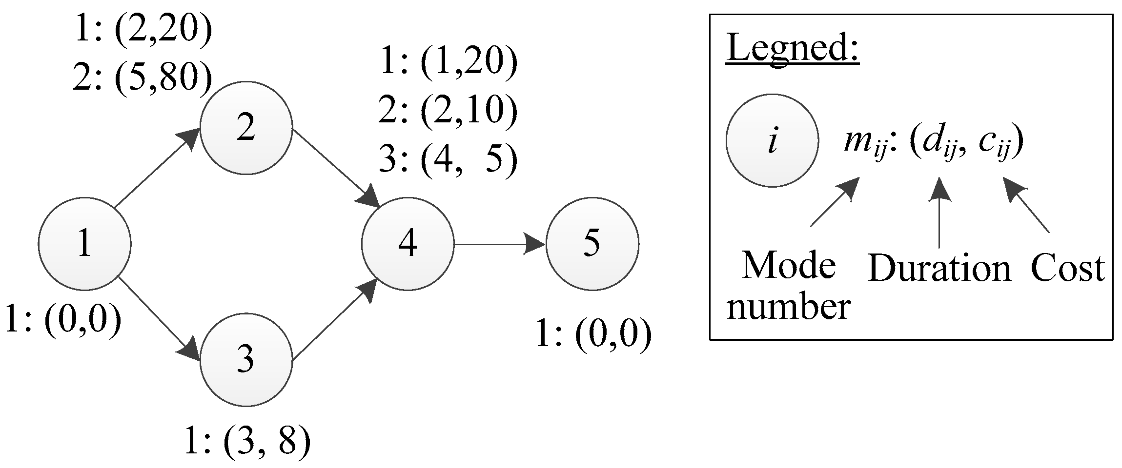
We use an example to illustrate the problem under consideration. Figure 1 shows a project network, in which each node has a corresponding activity number placed inside the node. For each activity, its modes are shown next to the node. The activities 1 and 5 are two dummy activities and have only one mode with zero duration/cost. Activity 2/3/4 has 2/1/3 mode(s), respectively.

There are six mode combinations for the example project. In other words, there are six solutions (mode assignment vectors) in total for this DTCTP-C instance. In Figure 2, the six solutions are represented in a two-dimensional objective space. The number besides each point shows the corresponding project makespan, cost, and mode assignment vector, respectively. The DTCTP-C aims to find the Pareto-optimal solutions which have been associated to the points P₁, P₂, P₃, P₅ and P₆ in Figure 2. Figure 2 also shows the Pareto frontier.

3. Bi-Objective Hybrid Genetic Algorithm

NSGA-II is a fast and elitist multi-objective algorithm that aims at obtaining good approximations of the non-dominated set of solutions [20,23,24,25]. In order to exploit the knowledge of the DTCTP-C, we introduce a critical path based crossover operator into the NSGA-II. The resulting algorithm is a bi-objective hybrid genetic algorithm (BHGA). Unlike the standard crossover operators which tend to randomly choose parts of the good solutions without any guarantee, our critical path based crossover operator can guarantee the offspring inherit the parts of the good solutions that contribute most to the objectives.

3.1. Schedule Encoding and Decoding

As mentioned in Section 2.1, a schedule can be determined by a mode assignment vector. Therefore, in the BHGA, a mode assignment vector $m=\left(m_1,m_2,\dots ,m_n\right)$ is used as a chromosome. The length of each chromosome is $n=\left|N\right|$. Each gene $m_i\in M_i \left(i\in N\right)$ in the chromosome corresponds to a mode of activity i. Note that since the dummy start and end activities have zero duration/cost, their modes are always unchanged in the BHGA.

Once a mode assignment vector (chromosome) is given, the baseline schedule $S^B=\left(s_1,s_2,\dots ,s_n\right)$ can be obtained by calculating the earliest start time of each activity in accordance with the CPM. In this way, a chromosome is decoded into a schedule.

With the above-mentioned schedule encoding and decoding mechanisms, given a chromosome, the corresponding objective function values (project duration and cost) can be calculated according to Equations (1) and (2). The fitness of a chromosome is represented by their non-domination rank (see next section).

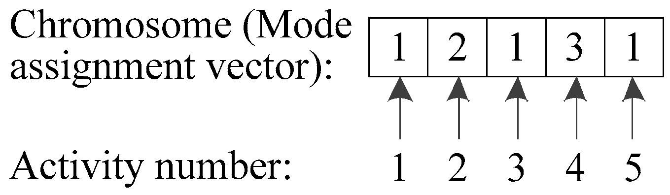
Consider the example project in Figure 1, a possible chromosome for this project is shown in Figure 3. The length of this chromosome is equal to the number of activities, i.e., 5. Each gene corresponds to a mode number. For example, the mode number of activities 3 and 4 are 1 and 3, respectively. We can get the baseline schedule (0, 0, 0, 5, 9) by decoding this chromosome. The resulting project duration and cost are 9 and 21, respectively.

3.2. Selection Operator

The binary tournament selection operator is used for selecting parent chromosomes. Two chromosomes are randomly chosen and the one with a lower non-domination rank is added to the matting pool. However, if both chromosomes have the same rank, the one with a greater crowding distance value will be chosen.

In NSGA-II, the non-domination rank of each chromosome is obtained by the fast non-dominated sorting approach [20]. Assume that the current population size is P, we find out all the non-dominated chromosomes and put them into the non-dominated set F₁ with rank 1. Then, we find out the non-dominated chromosomes from the remaining population and put them into the non-dominated set F₂ with rank 2. Repeat the process until all chromosomes are put into the corresponding non-dominated set F_p with rank p. By doing so, the population is divided into p (p ≤ P) disjoint sub-populations (non-dominated sets) and satisfies the condition that the non-dominated set with a smaller index dominates the non-dominated set with a larger index (i.e., $F_i$ dominates $F_j$, if $i<j$).

For chromosomes with either the smallest or the largest function values, their crowding distances are infinite. For other chromosomes, crowding distance is defined as the absolute normalized difference between the objective function values of two adjacent chromosomes. Therefore, the chromosomes with greater crowding distance value have more opportunities to be involved in the evolution process, which can maintain the population diversity.

3.3. Critical Path Crossover Operator

The crossover operator ensures that the good characteristics of the parent chromosomes can be inherited by the offspring. Given a chromosome, the corresponding project duration is determined by the critical path length. In the DTCTP-C, a short critical path length and a low total cost are desirable characteristics in a chromosome. However, shorter project duration is usually accompanied by higher project cost. Therefore, it is not always reasonable to transmit all activities on the critical path to the offspring. Instead, we set a threshold $\tau$ that determines the number of critical path activities transmitted to the offspring. In doing so, we might generate offspring with satisfying performance in both project duration and cost.

Based on the above observations, we develop a critical path crossover operator and the procedure is shown in Algorithm 1. In the critical path crossover operator, we first define the critical path ratio (CPR) as the proportion of the critical activities in a chromosome i, i.e., ${\mathrm{CPR}}_i=N_c/N$, where $N_c$ is the number of critical activities in the corresponding schedule after decoding chromosome i. Each chromosome is chosen for crossover with probability P_c according to tournament selection. Given two chromosomes to be crossed, we select the one with shorter (longer) makespan as the father (mother) chromosome. The son chromosome is generated in the following way: the value of the threshold $\tau$ for the CPR is randomly selected from the interval [l, u] ($0<l<u<1$, l and u are parameters and need to be determined by users). If the CPR of the father chromosome is less than $\tau$, then the son inherits all critical activities of the father, and the mother determines the remaining positions. Otherwise, the son only inherits $100\times \tau \%$ of critical activities of the father, and the mother determines the remaining positions. In order to ensure the diversity of the offspring, the daughter is generated in such a way that the daughter inherits the non-critical path activities of the mother chromosome and the father determines the remaining positions.

Algorithm 1. The Critical Path Based Crossover Operator.

Step 1: Given two chromosomes, select the one with shorter (longer) makespan as the father (mother) chromosome. Step 2: Compute the critical path ratio (CPR) for the father chromosome CPRf. Step 3: Generate the son chromosome. Choose $\tau$ randomly from the interval [l, u]. If CPRf < τ Put the genes that lie on the critical path of the father chromosome to the corresponding positions of the son chromosome. Else Select $100\times \tau \%$ of critical activities randomly from the father chromosome and put them to the corresponding positions of the son chromosome. End if The remaining positions of the son are determined by the corresponding genes of the mother chromosome. Step 4: Generate the daughter chromosome Put the genes that lie on the non-critical path of the mother chromosome to the corresponding positions of the daughter chromosome. The remaining positions of the daughter chromosome are inherited from the corresponding genes of the father chromosome.

3.4. Mutation Operator

In our algorithm, one-point mutation is used. Each chromosome has a probability P_m to be selected to mutate. For the chosen chromosome, one of its genes is randomly selected and its value is randomly changed to a different mode.

3.5. Algorithm Framework

In the BHGA, initial populations are generated randomly. In each iteration of the BHGA, the genetic operators (i.e., selection, crossover, and mutation operators) are applied to the chromosomes. The chromosomes with better fitness values have a higher chance to survive and enter next iteration. After a given number of iterations, the remaining populations will belong to or be close to the Pareto optimal set. The framework of the BHGA is described in Algorithm 2.

Algorithm 2. The Framework of the BHGA.

Step 1: Initialization. Generate the initial population P with size N randomly. Compute the objective function value for each chromosome of P. Step 2: Fast non-dominated sorting. Perform fast non-dominated sorting on the initial population P. Compute the rank and the crowding distance for each chromosome of P. Step 3: Genetic operation. Select N/2 chromosomes from P using binary tournament, resulting in the population Q. Generate offspring population R by performing the critical path crossover and mutation operator on Q. P’ $\leftarrow$ P ∪ Q. Perform fast non-dominated sorting on population P’. Update P by selecting N best chromosomes from P’ based on the rank and the crowding distance. Step 4: If the maximum number of generations is not reached, then go to Step 3; else: return P.

4. Steepest Descent Heuristic

The basic idea of our steepest descent heuristic is as follows. The solution space of the DTCTP-C could be divided into different parts in terms of the project deadline. For a given project deadline, we are able to find a solution with minimum project cost (this corresponds to solving a DTCTP-D). For a well-chosen project deadline, the resulting project duration and cost are most likely non-dominated. Hence, in this section, we obtain efficient solutions for the DTCTP-C by iteratively solving the DTCTP with different deadlines (i.e., DTCTP-D). In each iteration, given a project deadline, the solution that minimizes the total project cost is determined with the steepest descent search procedure presented in this section. Then the resulting solution is used as a start point for the next iteration. The solution returned by each iteration is (appropriately) Pareto-optimal.

4.1. Algorithm Framework

The steepest descent heuristic mainly consists of two stages: an initialization stage and a steepest descent search stage. Algorithm 3 gives the framework of our steepest descent heuristic. In Algorithm 3, a solution is also represented by a mode assignment vector m = (m₁, m₂, …, m_n) which specifies the execution mode m_i for each activity i.

In the initialization stage, the modes of each activity are sorted in the non-decreasing order of durations and labeled from 1 to |M_i|. The initial solution (mode assignment) m is generated by setting the mode of each activity at their crash mode m^crash = (1, 1, …, 1)_n. In the crash mode, all activities are set to their shortest duration. The normal mode m^normal in which all activities are set to their normal modes (longest duration) and the crash mode m^crash are obviously two efficient solutions. Therefore, they are added to the efficient set E. ITER is a predefined number used to control the number of repetitions of the steepest descent search in stage 2.

Algorithm 3. The Framework of the Steepest Descent Heuristic.

Stage 1: Initialization. For each activity i, sort its modes in the order of nondecreasing duration and label the resulting modes from 1 to |Mi|. m$\leftarrow$mcrash. E$\leftarrow$ {mcrash, mnormal}. ND$\leftarrow$ {(t(mcrash), c(mcrash)), (t(mnormal), c(mnormal))}. step$\leftarrow$$\lfloor \left(t\left(m^{\mathrm{normal}}\right)-t\left(m^{\mathrm{crash}}\right)\right)/\mathrm{ITER}\rfloor$. δ$\leftarrow$t(mcrash) + step. Stage 2: Iterative steepest descent. For i = 1 to ITER m’$\leftarrow$sd_search(m, δ). δ $\leftarrow$ t(m′) + step. if c(m’) $\le$ c(m) then E $\leftarrow$ E ∪ {m’}. m$\leftarrow$m’. End for For each m $\in E$ calculate t(m), c(m). ND$\leftarrow$ND ∪ {(t(m), c(m))}. End for Return efficient set E and non-dominated set ND.

In the second stage, the steepest descent search is repeated for ITER times to iteratively solve the DTCTP-D(δ) with different deadline δ. These deadlines are determined as follows. In the DTCTP, we can obtain the longest (t(m^normal)) and shortest project makespan (t(m^crash)) by choosing the normal and crash mode, respectively. Let the time increment $step=\lfloor \left(t\left(m^{\mathrm{normal}}\right)-t\left(m^{\mathrm{crash}}\right)\right)/\mathrm{ITER}\rfloor$. Then, in each iteration, the project deadline δ will be updated by adding step to the current deadline δ which is calculated according to the current mode assignment.

In each iteration of Stage 2, the specific DTCTP-D(δ) is solved by the steepest decent search procedure ‘sd_search( )’. ‘sd_search( )’ returns a mode assignment with minimum total project cost. After completing all iterations, we obtain the set of efficient solutions E and the corresponding non-dominated set ND. It can be observed that ITER (or step) determines the value of different project deadlines and hence it has an influence on the quality and quantity of the solutions in E.

4.2. Neighborhood and the Steepest Decent Search Procedure ‘sd_search( )’

We construct the neighborhood of a specific mode assignment vector m = (m₁, m₂,…, m_n) by changing the mode m_i of each activity i to its right adjacent one m_i′, i $\in$ N (m_i′= m_i + 1). We call this operation right move. Because the modes of each activity are already sorted in the non-decreasing order of durations (this also leads to a decreasing order of cost), the right move guarantees that the resulting total project cost satisfies c(m′) ≤ c(m′). The maximum number of possible moves equals $n$.

Given a mode assignment m, all of its neighbors are evaluated and then the one that yields the biggest reduction in cost without violating the project deadline constrains is chosen as the updated starting solution. In order to avoid calculating critical path for every move, we determine whether the project deadline constraint is violated in the following way. For an activity on the critical path, it is allowed to move to its neighbor mode, only when the difference between the activity’s neighbor duration and current duration is less than the difference between the project deadline and critical path length. For an activity that is not on the critical path, it is allowed to move to its neighbor mode, only when the difference between the activity’s neighbor duration and current duration is less than the difference between the project deadline and critical path length plus the activity’s total float. In doing so, certain computational time can be reduced.

If the neighborhood is examined entirely without any improvement, we have found a local optimum and terminate the search procedure.

In Algorithm 4, we give the pseudo-code for the steepest decent search procedure ‘sd_search( )’. CPL(m) is the critical path length that is calculated based on the mode assignment m. CA(m) is the set of activities that lie on the critical path(s) given the mode assignment m. Best_activity represents the activity that leads to the best improvement in the total project cost if a right move is performed on this activity. CB is the current best improvement value of the total cost. TF(i) represents the total float of activity i.

Algorithm 4. The Steepest Decent Search Procedure.

procedure sd_search(m, δ) best_activity $\leftarrow$ 0. Repeat   CB $\leftarrow$ 0.   Δd $\leftarrow$ δ $-$ CPL(m).   For each activity i and its current mode number mi     If i $\in$ CA(m) and $m_i\ne 1$ and $d_{i(m_i+1)}-d_{i{m}_i}<\mathsf{\Delta }d$       If $c_{i{m}_i}-c_{i(m_i+1)}>CB$         $CB\leftarrow c_{i{m}_i}-c_{i(m_i+1)}$.         best_activity $\leftarrow$ i.       End if     End if     If $i\notin$ CA(m) and $m_i\ne 1$ and $d_{i(m_i+1)}-d_{i{m}_i}<\mathsf{\Delta }d+TF(i)$       If $c_{i{m}_i}-c_{i(m_i+1)}>CB$         $CB\leftarrow c_{i{m}_i}-c_{i(m_i+1)}$.         best_activity $\leftarrow$ i.       End if     End if   End for   If best_activity $\ne$ 0 then mbest_activity $\leftarrow$ mbest_activity + 1. Until CB == 0 m $\leftarrow$ (m1, m2,…, mn). Return m.

4.3. Example

In this section, we use the example of Figure 1 to illustrate our steepest descent heuristic. We will let the steepest descent heuristic iterates three times (i.e., ITER = 3). The three iterations correspond to three rectangles (labeled with “Iteration 1/2/3”) that are shown in Figure 4. Figure 4 is created by adding the three rectangles to Figure 2. Each rectangle is associated with a project deadline and hence resulting in a DTCTP-D. In each iteration, a mode assignment vector will be used as the input, and all of its neighbors (associated with each rectangle) will be evaluated without violating the project deadline constraints. In other words, we need to find a mode assignment that minimizes the project cost given the project deadline specified by each rectangle.

As shown in Figure 4, points P₁ and P₆ correspond to crash mode and normal mode, respectively. Therefore, P₁ (corresponds to the mode (1, 1, 1, 1, 1)) and P₆ (corresponds to the mode (1, 2, 1, 3, 1)) are selected as two efficient solutions and added to the non-dominated set in the initialization stage.

Then the second stage which consists of three iterations begins. In Iteration 1, the project deadline is set to 6. The crash mode P₁ (1, 1, 1, 1, 1) is used as the initial solution. According to the definition of the right move given in Section 4.2, P₂ and P₃ are two neighbors of P₁. Since selecting P₃ will yield the biggest reduction in cost (48 − 36 = 12) and the total cost of P₃ (which is 36) is lower than that of P₁ (which is 48), we add P₃ to the non-dominated set, and P₃ will be the input of the second iteration.

In Iteration 2, the project deadline is 8. P₃ has only one neighbor P₅ and the total cost of P₅ (which is 26) is lower than that of P₃ (which is 36). Hence P₅ is added to the non-dominated set and will be the input of the next iteration. In the last iteration, there is only one solution P₆. Because P₆ corresponds to the normal mode and has been added to the non-dominated set in the initialization stage, there are no other solutions to evaluate and the steepest descent heuristic terminates.

In this example, the steepest descent heuristic found four efficient solutions (P₁, P₃, P₅, and P₆) and only P₂ is missed.

5. Computational Experiments

We have randomly generated a large number of problem instances to compare the performance of our algorithms. All of our algorithms are implemented in Matlab version R2010b and run on an Intel Core i5 2.40 GHz portable computer equipped with Windows 7. It is necessary to note that there is no research that has reported computational results for the large-scale DTCTP-C. Therefore, we only compare the performance of our two algorithms and our results can be served as the benchmark for future research.

5.1. Problem Instances Generation

In order to evaluate our algorithms, RanGen2 [26,27], which can generate strongly random networks in activity-on-the-node format, is used to construct 600 test instances using the parameter settings in

Table 1. The parameter settings of the problem instances.

Number of activities	100; 200; 300; 400; 500
Number of modes	Fixed at 4; 8; or randomly chosen from the interval [4, 20]; [8, 30]
I2	0.3; 0.5; 0.7
Activity durations	Randomly selected from the interval [1, 50]
Activity normal costs	Randomly selected from the interval [1, 10]
Slope	Randomly selected from the interval [1, 8]

. RanGen2 uses the serial/parallel indicator (I2) to measure the topological structure of a network. I2 measures the closeness of a network to a parallel or serial graph, ranging from 0 (indicating completely parallel) to 1 (indicating completely serial). For more information about the I2 indicator, we refer to Valadares Tavares et al. [28]. Specifying 5 settings for the number of activities, 4 settings for the number of execution modes, and 3 settings for the I2, we generated 10 problem instances for each of the 5 × 4 × 3 parameter settings, resulting in 600 instances in total.

In DTCTP, the types of cost functions could be linear, convex, concave, or random. We focus on the random one which is more general [26]. Following Demeulemeester et al. [26], the modes of an activity are generated in the following way: Firstly, the number of modes |M_i| is determined according to the modes parameter shown in Table 1. Then, |M_i| different values are randomly chosen from the discrete uniform distribution [1, 50] as the durations and are sorted in ascending order (d_i|Mi|, d_i(|Mi|−1),…, d_i1). In order to generate activity cost, starting with the normal duration mode d_i|Mi|, its corresponding cost c_i|Mi| is randomly chosen from the discrete uniform distribution [1,10]. By randomly choosing a slope s from the discrete uniform distribution [1, 8], we can calculate the cost of the next mode as c_i(|Mi|−1) = c_i|Mi| + s × (d_i|Mi| − d_i(|Mi|−1)), and we repeat this stepwise procedure until the mode corresponding to the maximum cost is reached.

5.2. Parameter Settings of the Algorithms

There are multiple settings of the parameters of our algorithms. For the BHGA, the parameters include: the threshold $\tau$ in the critical path crossover, crossover probability, mutation probability, population size, and the maximum number of generations. In our preliminary experiments, we found that fixing the first three parameters as the following values is decent enough to produce good results:

• Threshold $\tau$ is randomly chosen from the interval [0.3, 0.9].
• Crossover probability = 0.8.
• Mutation probability = 0.2.

For the remaining parameters of the BHGA, assigning two settings for the population size, and two settings for the maximum number of generations (as shown in

Table 2. The parameter settings of the algorithms.

BHGA1
Population size	50
Number of generations	50
BHGA2
Population size	50
Number of generations	100
BHGA3
Population size	100
Number of generations	50
BHGA4
Population size	100
Number of generations	100
SD1
Number of iterations	50
SD2
Number of iterations	100

), we therefore obtain four variants of the BHGA: BHGA1, BHGA2, BHGA3, and BHGA4. For the steepest decent heuristic, the maximum number of iterations (ITER) is the only parameter and is assigned two settings (as shown in Table 2). Hence, we obtain two variants: SD1 and SD2.

5.3. Experimental Results

In order to evaluate the performance of our six algorithms, we calculate the following metrics for each algorithm over all instances: the CPU time and the coverage metric e. In our experiment, the exact Pareto-optimal solutions are hardly known since the scale of the test instances is large. In this case, the coverage metric e which measures the percentage of efficient solutions in the obtained efficient set E that is produced by a specific algorithm is a suitable alternative. For a given algorithm ALG ($ALG\in \left\{\mathrm{BHGA}1,\mathrm{BHGA}2,\mathrm{BHGA}3,\mathrm{BHGA}4,\mathrm{SD}1,\mathrm{SD}2\right\}$), the corresponding coverage metric e(ALG) is calculated as [29]

$$e\left(ALG\right)=\frac{\left|E\left(ALG\right)\cap E\right|}{\left|E\right|}$$

(7)

where E(ALG) is the efficient set obtained by algorithm ALG. Efficient set E is obtained by removing the dominated modes from the union set E(BHGA1) ∪ E(BHGA2) ∪ E(BHGA3) ∪ E(BHGA4) ∪ E(SD1) ∪ E(SD2). Obviously, the coverage metric value ranges from 0 to 1. For a specific algorithm, the more efficient solutions it contributes, the closer its coverage metric value will be to 1.

Table 3. The average CPU time of different algorithms (in seconds).

	BHGA1	BHGA2	BHGA3	BHGA4	SD1	SD2
All instances	5.29	10.19	14.32	28.98	4.19	4.49
Number of activities
100	2.93	5.98	8.07	17.07	0.65	0.73
200	4.01	8.09	10.11	22.22	1.89	2.01
300	5.31	10.28	14.38	27.54	3.63	4.00
400	6.33	12.03	17.54	34.26	5.87	6.24
500	7.87	14.56	21.51	43.83	8.90	9.45
Number of modes
4	5.27	10.20	14.31	28.99	1.42	1.63
8	5.23	10.20	14.42	28.84	3.05	3.30
[4,20]	5.36	10.18	14.33	29.11	4.68	5.04
[8,30]	5.32	10.17	14.23	28.99	7.61	7.97
I2
0.3	4.68	9.30	13.34	27.03	4.01	4.33
0.5	5.26	9.84	14.12	28.20	4.14	4.40
0.7	5.94	11.42	15.51	31.72	4.42	4.73

presents the average CPU time over all problem instances solved by each of the six algorithms.

Table 4. The mean, median, and IQR of the coverage metric e for different algorithms.

		BHGA1	BHGA2	BHGA3	BHGA4	SD1	SD2
All instances	Mean Median IQR	0.04 0.03 0.03	0.05 0.04 0.04	0.13 0.12 0.13	0.23 0.22 0.20	0.12 0.10 0.12	0.46 0.46 0.30
Number of activities
100	Mean Median IQR	0.03 0.03 0.02	0.05 0.04 0.03	0.15 0.13 0.10	0.33 0.29 0.32	0.13 0.11 0.14	0.35 0.37 0.31
200	Mean Median IQR	0.03 0.03 0.02	0.04 0.04 0.02	0.13 0.10 0.11	0.22 0.21 0.19	0.13 0.11 0.09	0.48 0.51 0.27
300	Mean Median IQR	0.03 0.03 0.03	0.05 0.05 0.04	0.14 0.13 0.16	0.22 0.26 0.25	0.12 0.10 0.13	0.47 0.44 0.34
400	Mean Median IQR	0.03 0.03 0.02	0.04 0.04 0.03	0.12 0.11 0.10	0.18 0.16 0.14	0.12 0.11 0.11	0.53 0.53 0.20
500	Mean Median IQR	0.04 0.04 0.03	0.05 0.05 0.04	0.14 0.14 0.15	0.22 0.25 0.25	0.11 0.09 0.10	0.46 0.41 0.38
Number of modes
4	Mean Median IQR	0.02 0.02 0.02	0.04 0.03 0.03	0.08 0.07 0.08	0.21 0.17 0.21	0.14 0.10 0.16	0.55 0.59 0.28
8	Mean Median IQR	0.03 0.03 0.03	0.05 0.04 0.04	0.13 0.12 0.13	0.23 0.20 0.21	0.13 0.11 0.10	0.47 0.46 0.29
[4,20]	Mean Median IQR	0.04 0.04 0.02	0.05 0.05 0.04	0.16 0.16 0.14	0.27 0.25 0.21	0.11 0.09 0.11	0.40 0.39 0.31
[8,30]	Mean Median IQR	0.04 0.04 0.03	0.06 0.05 0.03	0.16 0.16 0.10	0.24 0.24 0.20	0.11 0.10 0.10	0.42 0.41 0.25
I2
0.3	Mean Median IQR	0.03 0.02 0.02	0.04 0.03 0.02	0.07 0.16 0.07	0.11 0.10 0.09	0.18 0.18 0.12	0.60 0.62 0.17
0.5	Mean Median IQR	0.04 0.04 0.03	0.05 0.05 0.03	0.14 0.14 0.10	0.22 0.23 0.11	0.11 0.10 0.09	0.47 0.45 0.20
0.7	Mean Median IQR	0.04 0.04 0.03	0.06 0.05 0.04	0.19 0.20 0.12	0.37 0.35 0.16	0.07 0.06 0.06	0.30 0.28 0.16

has a similar format to Table 3 and shows the mean, median, and interquartile range (IQR) of the coverage metric e for different algorithms. As shown in the row labeled ‘All instances’ in Table 3 and Table 4, the proposed steepest decent heuristic (SD2) outperforms the BHGA (1–4) over all 600 problem instances in terms of computational time and coverage metric. For the steepest decent method, better results are obtained with a large number of iterations (SD2) and the required computational expense does not increase significantly. For the BHGA, a large population size and generation lead to better results (BHGA4) at the expense of more computational time.

According to the rows labeled ‘Number of activities’, ‘Number of modes’, and ‘I2’ in Table 3, we observe that the three factors have a negative impact on CPU time: the more complex the test instance, the more the average CPU time is required.

It can be seen from Table 4 that the number of activities has a weak impact on the coverage metric, and the impact is especially slight for the BHGA. However, the impact of the number of activities does not show a regular pattern for the SD2, which probably means that we need to adjust the number of iterations according to the number of activities. For both the BHGA and the SD, the impacts of both the number of modes and the I2 on the coverage metric are opposite. For the BHGA, the higher both the number of modes and the I2, the greater the number of efficient solutions obtained. However, the SD shows an opposite behavior. This is because the performance of the SD is affected by the parameter step which determines the project duration increment in each iteration. For a more complex instance, it is necessary to use a relatively small value for step. While in our experiments, the value of step is fixed for each instance.

Overall, the steepest descent heuristic SD2 obtains more efficient solutions than other algorithms in promising computational time. Specifically, our SD2 outperforms the BHGA in both solution quality and computation efficiency. Compared with the SD1, our SD2 produces much better solutions and the required CPU time has only slightly increased.

6. Conclusions and Future Research

Time/cost trade-offs in projects are concerned with building baseline schedules that minimize project duration and cost simultaneously. In this paper, we presented two bi-objective heuristic algorithms for solving large-scale DTCTP-C with the aim of obtaining a good appropriate efficient solution set. The first algorithm BHGA is based on the NSGA-II. We devise a critical path based crossover operator to further exploits the knowledge of the DTCTP-C and improve the searching efficiency of the NSGA-II. The second algorithm is a steepest descent heuristic which generates efficient solutions by iteratively solving the DTCTP with different deadlines. We design a specified neighborhood search procedure based on the steepest descent search logic. Computational experience on the randomly generated problem data set validated both algorithms. Computational results reveal that our steepest descent heuristic algorithm outperforms the BHGA in terms of both the computational time and the coverage metric.

For future research, it will be a promising topic to devise more efficient and effective meta-heuristics for the DTCTP. It will also make our algorithms more practical by integrating them into project management decision support systems.