Environment-Smart Agriculture and Mapping of Interactions among Environmental Factors at the Farm Level: A Directed Graph Approach

Abstract

Environment-smart agriculture (ESA) aims at sustaining increased agricultural production while limiting negative impacts on the environment. The present study develops an index of composite on-farm environmental impacts (COEI) as a proxy measure to evaluate ESA and validates the index by mapping interactions amongst agriculture related environmental impacts and potential constraints to practice ESA by using the directed graph approach. The cost of mitigation to practice ESA was calculated by estimating the cost of reducing on-farm environmental impacts by using the damage–cost method. The approach was empirically applied to a sample of 317 High Yielding Variety (HYV) rice farms from three intensive rice-growing regions of northwestern Bangladesh. Results showed that the use of chemical pesticides contributed towards higher level of uncertainty in practicing ESA than the use of chemical fertilizers, irrigation and household pollution. The combined effect of the influence from these factor interactions was estimated at 2.3, which falls in the critical region of influence and implies extreme level of uncertainty in practicing ESA. The cost of mitigating negative environmental impacts is higher for the problems of ‘decline in soil fertility’, ‘increases in crop diseases’ and ‘reduction in fish catch’ as compared to other soil and water related impacts. Policy implications include investments in addressing the problems of ‘soil fertility decline’, ‘increases in crop diseases’ and ‘reduction in fish catch’ and raising farmers’ awareness on using farm chemicals to promote ESA practices for HYV rice production.

1. Introduction

Impact on the environment is one of the predominant negative side effects of agriculture that pose uncertainties in practicing environment-smart agriculture (ESA) practice. Intensive application of farm chemicals in high yielding crop agriculture contaminates farm environment, causes loss of the natural ecosystems, and generates multidimensional negative externalities [1]. Consequently, the negative environmental impacts restrict an increase in agricultural production [2], which is one of the mainstays of environment-smart farming practice. At a smaller scale, e.g., at the farm level, ESA can be defined as a set of farming practices that minimize negative impacts on the farm environment and thereby sustain agricultural production and profit/income. The concept of ESA is inspired by the approach of climate-smart agriculture (CSA) [3,4]. Environment-smart agriculture (ESA) is concerned with environment friendly farming practices that can potentially minimize on-farm environmental impacts for a given agricultural system. Compared to CSA, ESA considers a set of environment-friendly farming practices, which potentially exert a minimum level of impact on the farm environment for a given agricultural system, while CSA deals with farming operations at a comparatively larger scale. The approach of CSA addresses the challenge for an agricultural system to reorient and transform its existing system for a changing climatic condition in a global context so that it can help in sustaining agricultural income or profit and support food security. In order to transform the present agricultural system to cope with the new climate, CSA is concerned with establishing three pillars: productivity, adaptation and resilience and mitigation [3,5]. Absence of one or more pillars will pose difficulties in promoting a CSA system. On the contrary, the ESA practices are concerned with limiting on-farm environmental impacts and sustainability in agricultural production at a local scale. For instance, agricultural practices that can reduce greenhouse gas emissions, negative impacts on either soil or water resources or both can be denoted as ESA practices. Presence of one or more of such agricultural practices in a given agricultural system, which lead to exerting less impact on the farm environment, can be denoted as ESA practices. Such agricultural practices will potentially contribute to increase in agricultural output and income or profit. In this respect, chemical-intensive modern agriculture, such as HYV crop cultivation, essentially requires to adopt farming practices in an environment-smart way. Some of the most important environmental impacts, such as the degradation of farmland soil and pollution of water sources are mainly caused by chemical-intensive farming practices [6,7,8]. For example, consistent use of excessive and overuse of chemical fertilizer contaminates soil and water bodies by emitting greenhouse gases (GHGs). In fact, agriculture is the second largest contributor to global GHGs [9]. The HYV crop (e.g., HYV rice) farmers do readily recognize the problems of soil fertility, soil hardness, soil erosion and contamination of water along with health risks arising as a result of using farm chemicals in their field and are also aware of experiencing subsequent decline in production [6,7,8]. Sabiha et al. [8] found that up to 69 percent of the theoretical maximum level of environmental impacts (including different soil and water related problems) can be caused due to HYV rice cultivation in selected areas of Bangladesh. Therefore, it is essential but challenging to simultaneously sustain growth in agricultural production and reduce the negative impacts on the farm environment.

The challenge of realizing increased crop production while limiting negative impacts of agriculture (i.e., practicing ESA) requires collective efforts of the government and the farmers. The expense of reducing environmental impacts implicit in the environmental policy actions must represent the cost generated by negative externalities. Farmers are also expected to share adaptation and mitigation responsibilities for reducing negative environmental impacts of agriculture. Small-holder and marginal farmers in developing countries mostly depend on local inputs and serve vital roles in growing crops and managing extraction of natural resources. Their awareness regarding the use of chemical inputs and modern farming technologies is important. On the contrary, prolonged overexploitation of the farm environment, soil and vegetation depletion, and lack of farmers’ awareness would work against practicing ESA. Therefore, farmers can augment the quality and availability of natural capital by making changes in their production decisions [10] and should embark on a transition process towards adopting environment-smart production practices. This requires evaluating the extent of challenges in practicing ESA through identifying environmental problems, which generate higher impacts and estimate adaptation and mitigation costs for reducing those particular adverse impacts. Also chemical-based farming technologies should be identified that are primarily responsible for deteriorating the state of the farm environment. In this connection, mapping of interactions of the factors of environmental impacts is important and can be presented by the directed graph approach, which expresses such factor interactions as behavioral relations. Additionally, interpretation of such behavioral relations, analyzed digitally by computer interface, would facilitate environmental policy makers to understand the cause and effect relationships amongst negative environmental impacts and resulting challenges for practicing ESA [11]. This paper focuses on these relevant aspects of evaluating the on-farm environmental impacts produced by chemical-intensive agricultural practices, which poses as a challenge to practice ESA.

Given this backdrop, the overall aim of this article is to assess the potential challenges for practicing ESA by investigating on-farm environmental impacts caused by producing chemical-intensive HYV rice and mapping interactions amongst these environmental factors. The specific objectives are to: (a) identify the major environmental impacts of chemical-intensive HYV rice agriculture that contribute highest extent of challenge to practice ESA; (b) formulate a composite on-farm environmental impact index as a proxy to measure the aggregate extent of constraints in practicing ESA; (c) validate the index by mapping the degree to which factors of chemical-intensive agriculture interacts with each other, affect the farm environment and causes difficulties for the farms to practice ESA; and (d) estimate the cost of mitigating and reducing on-farm environmental impacts. The contributions of our study to the existing literature on sustainability are as follows. First, we have developed a proxy index measure of environmental impacts to evaluate constraints of practicing ESA at the farm-level. Second, we have applied the damage–cost approach to estimate the cost of mitigating and reducing negative environmental impacts arising from conventional agriculture. And third, we have demonstrated how the directed graph approach can be applied to visualize the behavioral relations and/or interactions amongst environmental factors which pose constraints in practicing ESA at the farm-level.

The rest of the paper is organized as follows. Section 2 reviews the literature on environment-smart agriculture, mitigation expenses, valuing environmental pollution from agriculture and modeling of factor interactions in agriculture. It also describes the methodologies, the study area and the data. Section 3 presents the results and finally, Section 4 provides conclusions and draws policy implications.

2. Materials and Methods

2.1. Literature Review

Adverse environmental impacts arising from agriculture is the main reason why ESA practices are required and therefore, it is important to identify the interactions amongst various factors that influence the likelihood of practicing environment-smart farming at the local scale, i.e., at the farm level. For example, chemical-intensive high yielding crop agriculture primarily degrades on-site natural and environmental resources such as farmland soil and water sources and pollutes the atmosphere. This subsequently affects future production/yield or agricultural profit/income and thereby poses considerable challenges in practicing ESA. Research investigating on-farm environmental impacts arising in the form of emission and pollution and their counter-effects on agricultural production are quite important. Additionally, such negative externality could be internalised by estimating its mitigation costs in terms of monetary values. The exercise would assist in (private) decision-making for environmental impact mitigation. Farmers (or farms) would be able to take production decision by comparing the social cost (i.e., sum of external cost/mitigation expense and private cost) of other alternative environment-smart agricultural practices. This ensures social welfare and helps in achieving environmental sustainability in agriculture [12].

Studies on environment and agriculture have frequently confirmed that intensive agricultural practices have contributed substantially to increases in world food production over the past several decades [13]. However, it has also been revealed that, these intensive agricultural practices has started to alter the farm environment, restrict the flow of resource availability in agriculture and reduce agricultural production [14,15,16,17]. Accordingly, the environmental consequence of chemical-based intensive agriculture is a major concern. These consequences include destruction of beneficial insects, waterlogging and salinization of irrigated land, pollution of groundwater and rivers, poisoning of farm workers and emissions of GHGs [14,18]. Due to such environmental and climatic concerns, wide range of studies on CSA was conducted. However, farm-level research on ESA considering local scale of effect can be an important pathway towards achieving CSA that considers the consequence of a changing climatic condition at a global scale. A workable approach to study ESA at the farm-level production consists of evaluating the nature of the farming practices that are employed and whether individual farmers are making efficient use of natural resources in achieving their economic objectives [19]. For instance, an intensive farming practice, which is being operated by applying actual doses (instead of overdoses) of chemical fertilizers and following recommended level of pesticide application, can be identified as some of the ESA practices. Also, farming units, where farmers are aware of switching amongst available water sources for irrigation, practicing crop diversification, proper management of crop residues and conscious about health and safety issues, can also be considered as ESA practices. These ESA practices can positively influence production efficiency, environmental quality and, therefore, sustainability in production [20]. Farmers, who are less conscious of the benefits of ESA, not only amplify the environmental impact of their farming activity but also increase production cost by causing higher external cost and induce production inefficiency simultaneously [19]. Sherlund et al. [21] discussed that, in the absence of environmentally sustainable production conditions, the technical inefficiency estimates becomes contaminated and rises sharply. As environmental pressure increases, the production efficiency decreases because both the value of farm outputs decrease and input costs increase, which might adversely influence the potential for practicing ESA. Therefore, evaluating such effects of different environmental impacts and mitigation costs of reducing those impacts can be a useful tool to evaluate the prospect of undertaking ESA practices at the farm level. It can therefore be hypothesized that farms that release higher amount of environmental pollution would face greater challenges to reorient their farming practices in an environment-smart way. Thus the extent of the impact on farm environment can be used as a proxy measure to evaluate the potential to practice ESA at the farm level. While evaluating on-farm environmental impacts and factors responsible for such negative impacts, a couple of impact variables (e.g., carbon emission or nitrous oxide emission) are generally considered [22]. Multiple numbers of impact variables (i.e., more than ten individual impacts) are rarely evaluated in an aggregated form using farm level data. However, to do this, one need to aggregate various environmental impacts into a composite form, e.g., index of composite on-farm environmental impact (COEI). Such index is generally computed by normalizing different types of environmental impact measurement units following statistical procedure and application of weights and addition [23]. In this connection, validating the composite index would be of immense significance. More specifically, graphical representation of individual factors of on-farm environmental impacts and their interactions, which influences the potential to operate ESA practices, would satisfactorily validate their behavioural relationships in a simplified but informed manner.

Ramos-Quintana et al., [11] argue that the right approach of describing and representing an environmental issue (e.g., ESA) is to develop the behavioral relations (dependencies) between a source and a final target. Therefore, building a synergistic linkage among certain factors of on-farm environmental impacts is relevant, which allows identifying important factors both numerically and visually [11]. Representation of the factor behavior helps to assess environmental sustainability precisely [24]. Higher extent of dependency between influencing factors implies that the factors affect the state of an environmental issue highly. Therefore, in addition to measure a proxy index of evaluating ESA, this paper also focuses on validating the index by analyzing the inter-relations using an interaction graph of factors causing such environmental impacts.

The ESA mainly is concerned with mitigating on-farm environmental impacts. Monetary values of environmental impacts measured in terms of external cost can be a useful tool in estimating mitigation cost of these impacts. Three basic methods for converting environmental impacts into monetary values can be found in the literature depending on the nature of environmental phenomena being studied. These are: the damage–cost method, the avoidance-cost method and the collective consent to pay method [25]. The damage–cost method is appropriate for analyzing monetary values corresponding to the pollution caused to receptors (humans, flora and fauna). Such monetary value of the impact is calculated by estimating willingness to pay (WTP) of the polluter/sufferer for the remediation of negative environmental impact caused/incurred [25]. This approach provides information on the amount willing to be paid to reduce or mitigate the on-farm environmental impacts by using WTP measure [26]. Therefore, the damage–cost method can be used to analyze the mitigation cost of on-farm environmental impacts and so the cost of operating ESA practices successfully.

2.2. Methodology

2.2.1. The Proxy Indicator to Measure ESA

ESA aims to enhance the capacity of the agricultural farms to sustain yields and incorporating the potential for mitigation into strategies for environmental sustainability in agriculture [3]. At the local scale, ESA practices aim to tackle three main objectives: less greenhouse gas (GHG) emissions, generating lower impacts on soils, and reducing the level of water pollution. Therefore, farms that aim at maintaining these three environmental objectives can be deemed as operating ESA practices. On the contrary, farming practices those have higher risks of releasing GHGs, generating negative impacts on farmland soil and causing pollution of agricultural water sources can create greater challenges and uncertainties for practicing ESA [27]. For example, chemical-based HYV crops may increase the yield but also impose negative impacts on the farm environment. Therefore, increase in production and farmer’s environmental awareness and decrease in GHG emission can be considered as the major three dimensions of practicing ESA for a farming system. These three dimensions of the ESA are closely interconnected. Farmers’ environmental awareness will help reducing GHG emission and water pollution, which helps sustaining growth in agricultural production and income. Measure of composite environmental impacts could therefore be an important proxy to represent the potential challenges for practicing ESA at the farm-level. Higher value of such composite impact would infer higher uncertainties/constraints for practicing ESA for a given agricultural system.

Table 1. Conceptualizing the ESA proxy measure.

Step (I)	Step (II)	Step (III)	Step (IV)	Step (V)
Identifying major aims of ESA practices at farm-level	Classifying basic categories of measurement components from Step (I)	Deriving relevant components of the ESA measure from Step (II)	Formulating and defining the proxy measure of ESA practices using relevant components from Step (III)	Validating the proxy index (COEI) of evaluating ESA defined in Step (IV)
Reduce GHG emissions	Emission-related impacts	Soil toxicity, Pollution of surface and ground water sources.	Composite index value of the selected on-farm environmental impacts (COEI) measures the potential for uncertainties/constraints to practice ESA. Farms having higher COEI value influence the potential of achieving ESA adversely.	Mapping interaction between the COEI and on-farm ESA potential by measuring their degree of influence using farm-level data.
Reduce impacts on the soil	Soil-related impacts	Soil stress factor, soil compaction, soil salinity.
Improve farmer’s perception on on-farm environmental impacts	Perception-based impacts	Soil fertility, crop diseases, pest attack, soil erosion, waterlogging, fish catch reduction, human health impact

Source: [3,4,28].

conceptualizes a five-step procedure of formulating and validating the proxy index of farm-level ESA potential.

2.2.2. Construction of the Composite On-Farm Environmental Impact (COEI)

Table 2. Construction of the impact variables and the COEI computation.

Impact Name	Function Type	Threshold Values		Optimal Range Scoring Function
		Lower (L)	Upper (U)
Soil fertility, crop diseases, pest attack, soil erosion, waterlogging, fish catch reduction, human health impact	Likert scale scoring using five-point scale.	0	1
Soil stress factor	MBF	2	36	$f\left(x\right)=0.9\left(\frac{x-L}{U-L}\right)+0.1$ if MBF $f\left(x\right)=1-0.9\left(\frac{x-L}{U-L}\right)$ if LBF
Soil compaction	MBF	100 psi	500 psi
Soil salinity	MBF	0.2 ds/m	2.0 ds/m
Water contamination/water pH, soil toxicity/Soil pH	MBF if pH > 7 LBF if pH < 7	7.05 4.0	8.5 6.9
Composite on-farm environmental impact (COEI)	Weighted summation of standardized values of the selected impacts

Note: Detailed description of the Likert scale and soil stress factor are given in Appendix A and B; MBF and LBF means ‘more is bad’ function and ‘less is bad’ function, respectively; x is the actual value of the impact, f(x) is the optimal range scoring function; resulted value of the f(x) is standardized value of the impact that ranges between 0.1 and 1. Source: [8,29].

describes those environmental impact variables used to construct the composite on-farm environmental impact (COEI) index and explains the aggregation procedure. The COEI aggregates the extent of major individual on-farm environmental impacts in a composite way. Actual values of the impact variables are standardized/normalized using optimal range scoring function. The COEI is defined as the weighted sum of those normalized impact values.

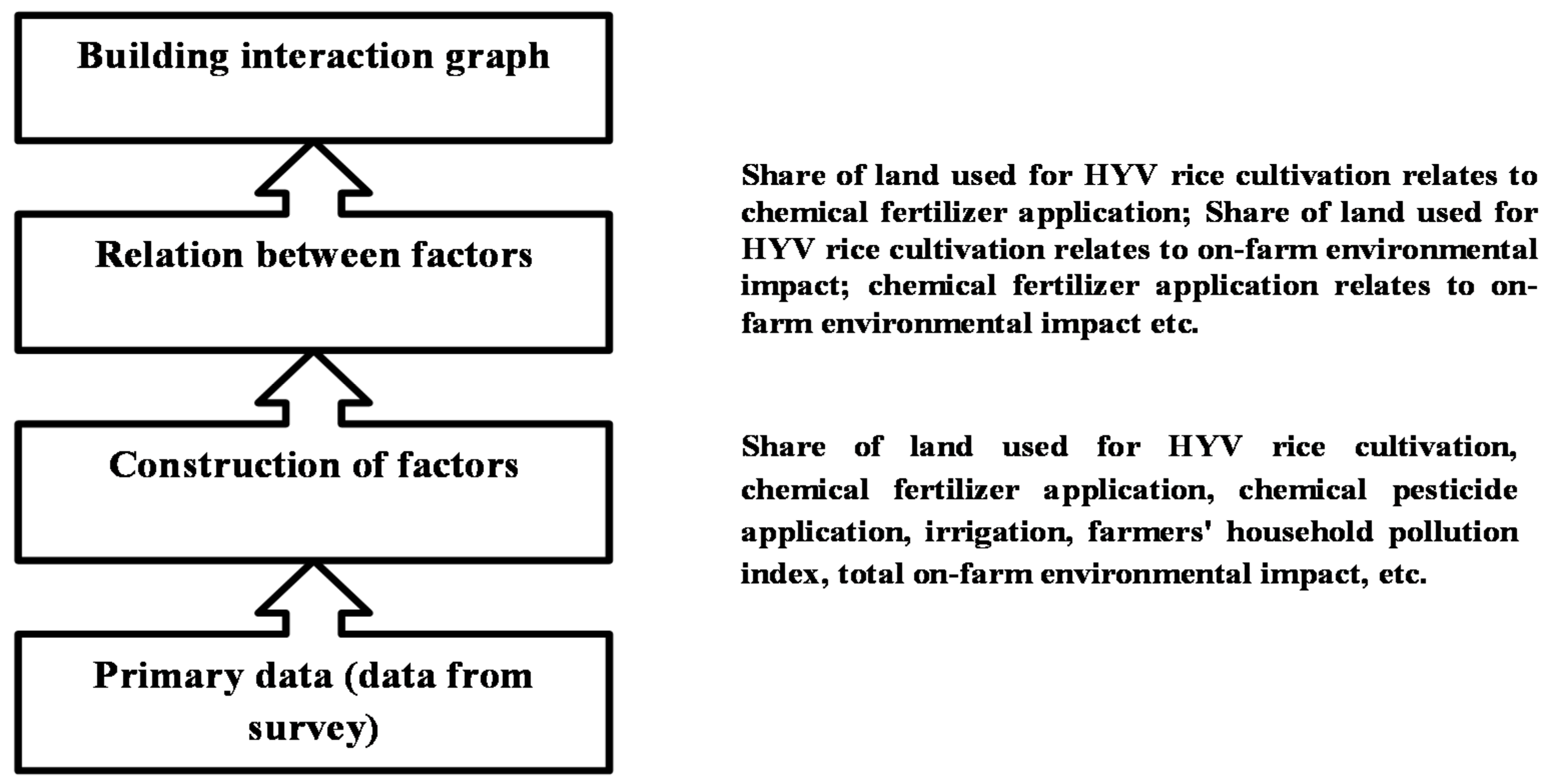
2.2.3. Validating the COEI as a Proxy Measure of Evaluating ESA: The Directed Graph Approach

The directed graph approach of the graph theory was used to draw causal network of relations among factors of on-farm environmental impacts and its degree of influence on the potential for ESA practices. Also, relevant mathematical operations were used to estimate numerical values of the level of interactions. The directed graph approach allows drawing links between factors in a synergistic way. A directed graph (or directed network) consists of a set of vertices (or nodes) and connects ordered pair of vertices, where all the edges are directed from one vertex to another [30,31]. Factors that pose challenges for practicing ESA through generating impacts on the farm environment, such as application of chemical fertilizers and pesticides, ground water extraction for irrigation and farmer’s household pollution index can be considered as vertices of the directed graph. Therefore, the directed graph approach can be used to build relevant links between these factors. Relation between factors was represented by an interaction graph, where two factors that are related to each other through a common variable. For example, the amount of chemical fertilizer application and environmental impact both relate to the share of land used for HYV rice cultivation. Based on such notion, a set of elementary relations can be expressed within the interaction graph. Then, these elementary relations can be combined to form complex relationships until one obtains a complete pictorial graph that adequately represents all factor interactions influencing the uncertainties/constraints in practicing ESA. Figure 1 shows the process of building and representing the graph of uncertainties/constraints in practicing ESA using the bottom-up approach [11]. The first tier is designed for collecting data on factors of on-farm environmental impacts. Second and third steps are to construct the factor variables and to build relations amongst those factors, respectively. The top of the graph-building process (i.e., the last tier) is for drawing the interaction graph that leads to the main issue (i.e., uncertainties/constraints in practicing ESA) under study.

2.2.4. Defining Factor Interactions: Understanding of the Relations

Table 3. Definition of factor relations and rules for their influence on target node.

No. of the Basic Relations	First	Second	Third
Definition of the basic relations	Factor A is related with factor B. [A→B]	If factor A is related with factor B and factor B is related with factor C, then factor A is related with factor C through B by transitivity rule [A→B, B→C then A→C]. The total extent of interaction is the multiplication of these two relations. (A→B) × (B→C) = (A→C)B	Factor A relates to factor C, factor B relates to factor C. [A→C, B→C]. Here two or more relations from different path direct to the same target node. The total extent of the factor interaction to the environmental issue is the sum of these two relations, which is (A→C) + (B→C).
Graph of basic relations
Definition of the rules	Slope A/B implies [A→B]	Slope A/B × Slope B/C implies [(A→C)B]	Slope A/C + Slope B/C implies [Total extent of factor interaction → the environmental issue under study (e.g., ESA)]
	Arctan of the slope value that ranges from angle 0° to 30° (segment 1), 31° to 60° (segment 2) and 61° to 90° (segment 3) means the relation (interaction) between factors influences the challenges of practicing ESA poorly, moderately and extremely respectively.

Source: Adapted and modified from Ramos-Quintana et al. [11].

describes the definition of factor relations and rules to measure their influence on the target node. Definition of the factor relations, as depicted in the interaction graph, should be established in a way so that it helps in understanding the overall potential to practice ESA through factor interactions. This facilitates operations combining relevant factor pairs and evaluating the extent of their influence on the state of the potential for practicing ESA at the farm level for a given agricultural system. The level of interaction between two factor variables was evaluated by analyzing their dependency ratio (i.e., slope). The slope indicates how one factor variable responds to a change in another factor variable, which can be read by its upward or downward directions. A set of rules is defined, which provide information on responses of both factors and allow comparison of their influence on the concerned environmental issue [11,31]. The definition of the rules should be based on the angle formed by the axes of the two factors, e.g., factor A and factor B. For example, if one unit changes in the value of the abscissa changes the value of the ordinate by more than one unit, then the arctan of the slope value of the curve tends to be close to the angle of 90°, which means that the interaction between these factors exert extreme influence on the potential to practice ESA (i.e., the final target node). A similar proportional change in two-factor variables implies moderate influence, while poor influence of the factor interaction on the target node was exerted when one unit change in abscissa changes the ordinate by less than one unit. Therefore, the angle ranges from 0° to 90° and divided into three segments. Definitions of the segment 1, 2 and 3 explain semantic meaning of the responses of the factor variables (Table 3).

2.2.5. Construction of the Farmer’s Household Pollution Index

As an important socioenvironmental factor, this article hypothesized that farmers who produce considerable amount of household pollution would rarely be aware of practicing ESA on their farms. Therefore, farmers’ environment-friendly lifestyle can be considered as a proxy of farmers’ environmental consciousness. Socioecological status was evaluated by many recent studies as an important factor determining natural resource management [32].

Table 4. Components of the FHP and activity weights.

	Environment Polluting Activity Weights (Ew)
Attributes (r)	(4) Least	(3) Good	(2) Better	(1) Best
House category	Clay	Straw	Half-concrete	Full-concrete
Sanitation	Open place	Temporary latrine	Sanitary latrine (without water seal)	Sanitary latrine (with water seal)
Access to health facility	Village doctor	Health center	Clinic	Hospital
Drinking water source	Pond/river	Well	Supply	Deep tube well
Household energy source	Timber/straw/cow dung/dried leafs/kerosene	Electricity	Biogas/natural gas	Solar power
Waste disposal	No specific place to dispose	Burnt	Buried	Specific place/waste bin

Source: Author’s own calculation.

describes construction of the farmer’s household pollution index (FHP). The FHP is computed by assigning weights on the farmers’ socioenvironmental living attributes (e.g., house category, sanitation status, access to health facility, pure drinking water source, household energy source and waste disposal system). A farmer with a FHP close to 1 (i.e., higher level of household pollution) is less likely to be conscious of on-farm environmental impacts and environment friendly farming practices (i.e., ESA)—a value of FHP close to 0 implies otherwise.

$${\mathrm{FHP}}_i={\displaystyle \sum }_{r=1}^{6}E{w}_r / 24$$

(1)

2.2.6. Mitigation Cost of Practicing ESA: The Distribution-Free Turnbull Estimator

The WTP measure of the damage–cost method was used to estimate the cost of mitigating on-site damage in terms of the monetary values of the negative impacts (externalities). This can be defined by farmers WTP values for mitigating/reducing on-farm environmental impacts and for adopting environment-friendly production practices. Usually, this approach induces survey questions that examine respondents’ WTP for environmental impact mitigation and evaluate its monetary values as external cost [33,34]. Consider M distinct randomly offered bid amounts (percentage of HYV rice farmers’ monthly income), indexed t_j for a set of 12 different environmental impacts. Randomly assigned bid amounts take on values: 5 percent, 6 percent, 7 percent, 8 percent, 9 percent, 10 percent, 12 percent, 13 percent, 14 percent, 16 percent, 18 percent, 19 percent and 20 percent. If the $i$th farmer agrees for a randomly offered bid to reduce a specific environmental problem, the WTP is greater than or equal to that offered bid, i.e., $WT{P}_i \ge t_j$, otherwise $WT{P}_i \le t_j$. Because WTP is unobservable to the researcher in advance, assume the WTP as a random variable with cumulative distribution function (CDF), $F_W\left(W\right)$ such that ${\mathrm{P}}_{\mathrm{r}}\left(\mathrm{WTP}\le t_j\right)=F_w\left(t_j\right)\left(=F_j\right)$ [35,36]. The present study uses the distribution-free Turnbull estimator [37] to measure the monetary values of the WTP. Potentially, the estimator makes minimal assumptions about the distribution of willingness to pay. It assumes monotonic CDFs for proposed bids, i.e., as the bid amount (percentage of farmers monthly income) increases, the number of ‘no’ responses to each bid for a given environmental impact increases. Imposing the monotonicity restriction, the log-likelihood maximization problem is given by Equation (2):

$$\begin{array}{c}\underset{F_1,F_2,\dots ,F_M}{\max }={\displaystyle \sum _{j=0}^M}[N_j\ln \left(F_j\right)+Y_j\ln \left(1-F_j\right)]\\ \mathrm{subject} \mathrm{to} F_j\le F_{j+1}| \forall j \end{array}$$

(2)

where $N_j$ and $Y_j$ are the number of ‘no’ and ‘yes’ responses to the bid $t_j$, respectively. Following Haab and McConnell [35,36], we express the Turnbull distribution-free estimator and define the expected lower bound willingness to pay, E_LB (WTP), along with the variance, $V\left(E_{LB}\left(WTP\right)\right)$, for M* distinct bids as follows (M* refers to particular bids after pooling due to the Turnbull monotonicity restriction):

$$E_{LB}\left(WTP\right)={\displaystyle \sum }_{j=0}^{M^{*}}{t}_j(F_{j+1}^{*}-F_j^{*}）$$

(3)

$$V(E_{LB}\left(WTP\right))={\displaystyle \sum }_{j=1}^{M^{*}}\frac{F_j^{*}\left(1-F_j^{*}\right)}{T_j+T_{j+1}}(t_j- t_{j-1})²$$

(4)

where $F_j^{*}$ is the pooled CDF value and $F_{j+1}^{*}-F_j^{*}$ is the respective probability density function (PDF) of the WTP for an environmental impact, i.e., the Turnbull estimate. $F_j^{*}=N_j+N_{j+1 }/ T_j+ T_{j+1}$ where, T_j is the total number of respondents offered the bid t_j By using data on the proportion of ‘no’ responses for a given impact, for each of the randomly assigned bid amount, we estimate the CDF followed by successive PDF. Given the monotonicity assumption, CDF values that break the monotonic order are pooled with the values from the previous bid. For a given environmental impact attribute in a particular study region, Equation (2) therefore calculates the lower bound willingness to pay, E_LB(WTP) (notation and definitions of Equations (2) and (3) are similar to Haab and McConnell, [35]).

As a non-parametric estimator, the Turnbull has a number of theoretical advantages over the parametric models [35]: (i) it provides an empirical distribution function with the necessary information to calculate a lower bound WTP and hence eliminates the variation due to functional form; (ii) it always results in a positive estimate of WTP and provides an ease of exercising econometric computation; (iii) it can be directly calculated from a data table of bids offered to the respondents, along with the number of both ‘no’ and ‘yes’ responses; and (iv) it potentially emphasizes the characteristic and implication of the CV questions and responses rather than its statistical interpretation. As a damage–cost method-based environmental impact valuation study, we therefore empirically estimate the WTP Turnbull values by applying Equation (3) separately for 12 selected environmental impacts and for an overall farm-level environmental impact.

2.2.7. Study Area and the Data

Bangladesh, as a developing economy, is currently experiencing negative environmental impacts caused by intensive cultivation practices. Primary data on HYV rice production, on-farm environmental impacts and farmers’ WTP for reducing or mitigating environmental impacts were collected from HYV rice farms in three intensive rice growing regions of northwestern Bangladesh. A total of 330 HYV rice farmers are randomly selected from the list of registered farm households provided by Agricultural Extension Service Offices (AESO). The sample size is calculated following Cochran [38] and Bartlett et al. [39]. All of the selected farmers were interviewed face-to-face, and 317 questionnaires were screened as effective, out of which 113 were from Rajshahi, 101 from Natore and 103 from the Pabna region.

Table 5. Descriptive statistics of the factor variables.

	Mean	Std. Dev.	Min	Max
Chemical fertilizers (CFR) (Kg per hectare)	555.25	118.4	296.52	3743.64
Chemical pesticides (CPS) (Kg per hectare)	11.86	2.74	0.74	49.42
Irrigation (IRR) (Ground water extraction hours per hectare)	289.36	33.7	108.73	593.05
Farmers household pollution index (FHP)	0.741	0.12	0.11	1
Proportion of land under HYV rice cultivation (PLH)	0.82	0.37	0.15	1
Composite on-farm environmental impact (COEI)	7.39	2.4	3.33	10.67

Source: Field survey by the authors.

shows descriptive statistics of the factor variables of the on-farm environmental impacts. On an average, farmers in the study area are using 555.25 kg of chemical fertilizers and 11.86 kg of chemical pesticide per hectare of land per crop season. Ground water extraction time for irrigation was recorded as 290 h per hectare of land per crop season. As the consequence of such intensive application of farm chemicals and high volume ground water extraction practices, average value of the composite on-farm environmental impact (COEI) is found as 7.39. This quantity is around 69.25 percent of the observed maximum COEI value and represents a considerable constraints and challenges for practicing ESA practices. In the farmland area, risks of environmental impacts and challenges for operating ESA practices are also caused due to farmers’ household pollution (FHP) factor. Mean value of the FHP index is estimated as 0.74, where 1 implies the maximum extent of the FHP index (Table 4) and higher challenges for ESA practices.

3. Results

3.1. Ranking of Individual Environmental Impacts Based on Standardized Scores

Table 6. Mean environmental impact scores by study regions.

Impact Names	Rajshahi	Pabna	Natore	All Region
SFP (problem of soil fertility)	0.67 (4)	0.72 (2)	0.58 (5)	0.66 (3)
PAP (problem of pest attack)	0.75 (2)	0.39 (6)	0.42 (6)	0.53 (6)
CDP (problem of crop diseases)	0.80 (1)	0.69 (4)	0.77 (3)	0.76 (1)
SER (soil erosion)	0.15 (9)	0.67 (5)	0.90 (1)	0.56 (5)
SCM (soil compaction)	0.49 (5)	0.34 (8)	0.29 (8)	0.38 (7)
SSL (soil salinity)	0.20 (8)	0.36 (7)	0.35 (7)	0.30 (8)
SSF (soil stress factor)	0.19 (10)	0.73 (1)	0.80 (2)	0.56 (4)
WLG (problem of water logging)	0.20 (7)	0.27 (9)	0.26 (11)	0.24 (9)
GWpH (ground water pH/water contamination)	0.10 (12)	0.10 (12)	0.29 (9)	0.16 (11)
RFC (problem of fish catch reduction)	0.74 (3)	0.70 (3)	0.73 (4)	0.72 (2)
HI (health impact)	0.25 (6)	0.17 (10)	0.28 (10)	0.23 (10)
SpH (soil pH/soil toxicity)	0.13 (11)	0.11 (11)	0.17 (12)	0.14 (12)

Note: Rank orders are presented in the parenthesis. Mean values close to ‘1′ imply highest impact (environmental problem). Source: Authors calculation from primary survey.

shows mean values of the standardized scores of environmental impact indicators classified by study regions. Standardized scores of the ‘increase in crop diseases’, ‘reduction in fish catch’ and ‘decline in soil fertility’ were found to be the top three impacts which have the highest extent of impacts for all regions. These environmental impacts affect considerably the potential for ESA practices. In the Rajshahi, Pabna and Natore study regions, impact values were found to be the highest for ‘crop diseases’, ‘soil stress factor’ and ‘soil erosion problems’, respectively. This might be due to the intensive application of farm chemicals and extensive irrigation practices used for HYV rice production.

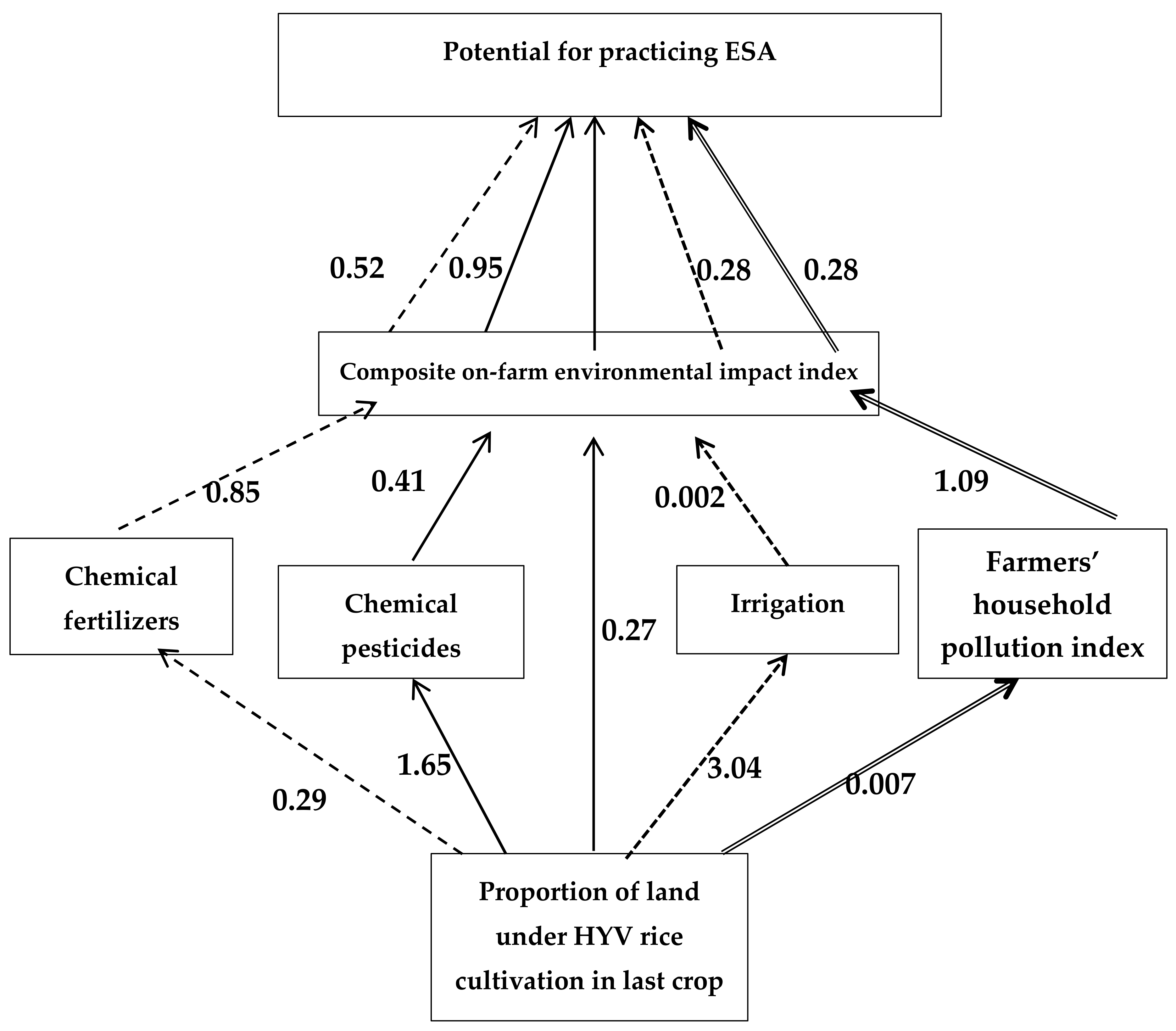
3.2. Analyzing Factor Interactions and Its Extent of Influence on ESA Practices

Table 7. Interaction between factors and their extent of influence.

No. of Operations	Interaction between Factors and Their Influence on the State of On-Farm Negative Externality	Extent of the Influence to Target Node (Negative Externality Condition)
1.	(ΔPLH→ΔCOEI) = 0.27	0.27 (≈15.1°)
2.	(ΔPLH→ΔCFR × ΔCFR→ΔCOEI) = (ΔPLH→ΔCOEI)ΔCFR = 0.29 × 0.85 = 0.25	(ΔPLH→ΔCOEI)ΔCFR + (ΔPLH→ΔCOEI) = 0.25 + 0.27 = 0.52 (≈27.47°)
3.	(ΔPLH→ΔCPS × ΔCPS→ΔCOEI) = (ΔPLH→ΔCOEI)ΔCPS = 1.65 × 0.41= 0.68	(ΔPLH→ΔCOEI)ΔCPS + (ΔPLH→ΔCOEI) = 0.68 + 0.27 = 0.95 (≈43.53°)
4.	(ΔPLH→ΔIRR × ΔIRR→ΔCOEI) = (ΔPLH→ΔCOEI)ΔIRR = 3.04 × 0.002=0.007	(ΔPLH→ΔCOEI)ΔIRR + (ΔPLH→ΔCOEI) = 0.007 + 0.27 = 0.28 (≈15.64°)
5.	(ΔPLH→ΔFHP × ΔFHP→ΔCOEI) = (ΔPLH→ΔCOEI)ΔFHP = 0.007 × 1.09 = 0.008	(ΔPLH→ΔCOEI)ΔFHP + (ΔPLH→ΔCOEI) = 0.008 + 0.27 = 0.28 (≈15.64°)
	Total extent of COEI influence on practicing ESA practices	2.30 (≈66.5°)

Note: ‘→’stands for ‘relates to’. Source: Authors’ calculation.

provides results of the relations between factors and their influence on practicing ESA practices at the farm level. The extent of the influence of each vertex (nodes: pair of related factors) to ESA is also calculated. The proportion of land used for HYV rice cultivation is considered as the factor, which directly relates with COEI. The proportion of land also relates to COEI through the application of chemical fertilizers, chemical pesticides, irrigation and household pollution index (based on transitivity rule). All these interactions are defined by rules of constructing relations between vertex pairs of the directed graph explained in Table 2. The extents of the influence on ESA due to interactions of factor variables were numerically estimated. The extent of the influence from first interaction (operation no. 1 in Table 7) is 0.27, while it is 0.52 and 0.95 for second and third interactions, respectively. The total extent of these interactions was calculated by summation of the slope values associated with each factor pair as shown in Table 6. The angle corresponding to the total slope value 2.3 is 66.5°, which falls within the segment 3 (definition of segment 3 is explained in Table 2). This implies that the total extent of the influence of factor interactions on the potential for practicing ESA practices is considerable. Therefore, if the extent of interaction between the factors falls within segment 1, segment 2 or segment 3, the implication is that such interactions cause high, medium or low level of challenges to practice ESA practices, respectively. It was revealed that the application of chemical pesticides positively relates to the COEI and affects the potential for ESA practices to a higher extent as compared to the other set of factor interactions. The interaction graph appropriately expresses these numerical results visually through mapping interactions [40]. Therefore, Figure 2 depicts how factors of on-farm environmental impact interact with each other and affect COEI. The directed graph (Figure 2) therefore validates the COEI as the proxy measure of ESA by mapping inter-relationship between these factors. These findings inform decision makers and the public that the necessity of managing environmental risks arising from chemical pesticide application is comparatively larger than other factors [41] and therefore poses greater uncertainties/challenges in practicing ESA.

3.3. Valuation of Mitigation Cost of ESA Practices

Table 8. Mitigation cost of on-farm environmental impacts.

	Rajshahi		Pabna		Natore		Three Region Average
	E(WTP)	BDT	E(WTP)	BDT	E(WTP)	BDT	E(WTP)	BDT
Soil fertility	13.48	4.67 (1)	7.20	2.62 (5)	11.53	3.83 (2)	10.74	3.71 (1)
	(0.86)		(0.76)		(0.89)
	[11.79, 15.17]		[5.71, 8.69]		[9.79, 13.27]
Pest attack	10.22	3.64 (3)	6.02	2.19 (6)	11.48	3.82 (3)	9.33	3.22 (3)
	(0.96)		(0.99)		(0.68)
	[8.34, 12.10]		[4.08, 7.96]		[10.14, 12.18]
Crop diseases	10.49	3.54 (4)	7.33	2.67 (4)	11.73	3.89 (1)	9.76	3.37 (2)
	(0.88)		(0.80)		(0.71)
	[8.76, 12.83]		[5.76, 8.89]		[10.33, 13.12]
Soil erosion	10.70	3.71 (2)	4.88	1.78 (9)	10.45	3.47 (5)	8.68	3.00 (5)
	(1.09)		(0.69)		(0.78)
	[8.56, 12.83]		[3.52, 6.23]		[8.92, 11.97]
Soil compaction	10.12	3.51 (6)	4.51	1.64 (11)	7.65	2.54 (9)	7.43	2.56 (10)
	(1.02)		(0.79)		(0.81)
	[8.12, 12.12]		[2.96, 6.05]		[6.06, 9.23]
Soil salinity	4.33	1.50 (12)	5.18	1.89 (8)	5.65	1.88 (11)	5.05	1.76 (12)
	(0.89)		(0.73)		(0.75)
	[2.59, 6.07]		[3.74, 6.61]		[4.18, 7.12]
Soil stress Factor	7.44	2.58 (8)	8.58	3.12 (2)	10.85	3.61 (4)	8.82	3.10 (4)
	(0.92)		(0.90)		(0.94)
	[5.64, 9.24]		[6.81, 10.34]		[9.01, 12.69]
Waterlogging	5.88	2.04 (10)	8.48	3.09 (3)	10.02	3.33 (6)	8.13	2.82(6)
	(0.70)		(0.73)		(0.94)
	[4.51, 7.25]		[7.04, 9.91]		[8.17, 11.86]
Water contamination	10.19	3.53 (5)	4.42	1.61 (12)	8.53	2.84 (7)	7.71	2.66 (7)
	(1.06)		(0.73)		(1.08)
	[8.11, 12.27]		[2.98, 5.85]		[6.41, 10.65]
Fish catch reduction	4.41	1.53 (11)	10.30	3.75 (1)	8.02	2.67 (8)	7.58	2.65 (8)
	(0.78)		(0.74)		(0.80)
	[2.88, 5.94]		[8.84, 11.75]		[6.45, 9.58]
Human health impact	9.84	3.41 (7)	5.73	2.09 (7)	6.81	2.26(10)	7.46	2.59 (9)
	(0.76)		(0.74)		(1.09)
	[8.35, 11.33]		[4.28, 7.18]		[4.67, 8.95]
Soil toxicity	7.40	2.57 (9)	4.67	1.70 (10)	5.39	1.79(12)	5.82	2.02 (11)
	(1.09)		(0.66)		(1.02)
	[5.26, 9.54]		[3.38, 5.96]		[3.39, 7.38]
Overall impact	8.12	2.82	5.29	1.95	5.84	1.94	6.42	2.23
	(0.78)		(0.83)		(0.92)
	[6.59, 9.65]		[3.66, 6.91]		[4.03, 7.64]
Farm size-wise mitigation expense
Large farms	13.48 (1.75)	4.67 (1)	6.4 (1.95)	2.33 (1)	5.80 (2.38)	1.93 (1)	8.56	2.98 (1)
	[10.05, 16.91]		[2.58, 10.22]		[1.14, 10.46]
Medium farms	6.32 (1.19)	2.19 (2)	6.4 (1.33)	2.33 (2)	5.05 (1.22)	1.69 (2)	7.60	2.07 (2)
	[3.98, 8.65]		[3.79, 9.01]		[2.65, 7.44]
Small farms	5.27 (0.50)	1.83 (3)	3.91 (0.61)	1.43 (3)	4.59 (0.67)	1.53 (3)	5.88	1.60 (3)
	[4.29, 6.25]		[2.71, 5.10]		[3.27, 5.90]

Note: E(WTP) unit is the percentage of farmer’s monthly income willing to pay for reducing or mitigating environmental impact. Standard errors are reported in parentheses. Ninety-five percent confidence intervals are reported beneath the standard errors in parentheses. BDT means Bangladeshi currency (Thousand Taka per farm household per one crop year). This amount represents the monetary value of adaptation and mitigation of on-farm environmental impacts. Rank orders of the expenses are reported in parentheses of BDT column. 1 USD = BDT 83.42 (Exchange rate of March 2018).

presents mitigation costs in terms of costs of environmental impacts. These amounts are represented by the E_LB (WTP) Turnbull estimates along with the respective standard errors calculated using Equation (4). The E_LB (WTP) estimates were converted into monetary values to calculate mitigation expense of each impact. Results revealed that mitigation cost in the Rajshahi region is highest for the problem of ‘decline in soil fertility’, while it is highest in Natore and Pabna for the problems of ‘increase in crop diseases’ and ‘reduction of fish catch’, respectively. This finding corresponds to Rahman [7], who noted that the HYV rice cultivation in Bangladesh results in ‘reduction in soil fertility’, ‘human health impact’, and ‘reduction in fish catch’ followed by ’crop diseases’ and ‘problems of pest attack’. Considerable disparity was found in the mitigation cost for overall impact attribute across farm size categories. It was revealed that the cost of reducing environmental impacts increases with an increase in farm size. That is, the large farms need to spend higher amount for mitigating environmental impacts than medium and small farms when overall impact is considered. These findings are consistent and comparable with the findings in the literature. For example, Ulimwengu and Sanyal [42] noted that external cost of reduction in soil fertility increases with an increase in farm size in Uganda. Angella et al. [43] found that the rice farmers asses USD 19.8 per hectare per season as mitigation cost caused in terms of a particular environmental impact in Uganda whereas Alhassan [44] reported the value of reducing environmental impacts of rice cultivation is USD 8.5 per hectare per year in Northern Ghana.

4. Conclusions

The main aim of this study was to evaluate the potential to practice ESA at the farm-level. This was done first by developing a proxy index (i.e., COEI) that measures the extent of challenges or constraints in practicing ESA. Then the index was validated by mapping behavioral relationships among environmental factors, which adversely influence the potential for ESA practices by using a directed graph approach. Then the cost of mitigation of those environmental impacts was estimated using the damage–cost method. The approaches were empirically applied to a sample of 317 HYV rice farmers from three intensive rice-growing regions of Bangladesh. Results revealed that the interaction between application of pesticides and the COEI caused the highest extent of constraints to practice ESA than the application of chemical fertilizers, extraction of water for irrigation and household pollution. The total extent of the influence from factor interactions is estimated at 2.3, which falls in the critical region (i.e., segment 3) and implies extreme extent of influence. The interaction map showed that farms with higher value of the COEI might face greater challenges to practice ESA. The environmental impacts arising from HYV rice agriculture can be mitigated by spending BDT 2230.00 (equivalent to USD 26.73) per farm per crop year in the study area. The cost of mitigation are higher for the problems of ‘decline in soil fertility’, ‘increase in crop diseases’ and ‘reduction in fish catch’ as compared to other on-farm environmental impacts. Regional variation exists in the cost of mitigation of specific type of environmental impacts. The cost of mitigation also varies by farm size categories.

A number of policy implications can be drawn from the results of this study. First, investment is needed to reduce the problems of ‘declining soil fertility’, ‘increase in crop diseases’ and ‘reduction in fish catch’. Agricultural extension services can play an important role in disseminating technological knowhow to farmers, which can be extended to include promotion of environment-smart production practices. The AESO can provide services on prohibition of applying overdoses of chemical fertilizers, enforcement of pesticide application according to recommended guidelines, raising awareness on the alternative uses of available water sources for irrigation, establishment of water reservoirs during the wet season and in low-land farm areas and regulations of safety issues regarding the use of farm chemicals etc. In particular, agri-environmental policy should be developed at the local level in environmentally critical regions. Provision and successful implementation of agricultural service schemes should advocate to reduce those negative environmental impacts which require highest cost for adaptation/mitigation as compared to other impacts in the study area. Second, dissemination of information aimed at raising awareness of the farmers on the benefits of reducing GHG emission, impacts on farmland soil and pollution arising from intensive HYV rice cultivation practices, particularly, from using farm chemicals. Bangladesh already provides special programs on farming technologies in national TV and popular radio channels, which needs to be modified to include information on the benefits of practicing ESA practices. Effective implementation of these policy measures will help to reduce the environmental impact footprint of intensive HYV rice cultivation in Bangladesh and promote ESA practices.

A limitation of the present study is that we have conducted our research in three major rice-growing areas of the country only, which is not nationally representative. Nevertheless, we have applied standard statistical procedure to draw samples so that the results derived from this study can be generalized for a wider context. However, future research could extend such study on a nationally representative sample, which will incorporate wider level of variation in the nature and magnitude of environmental issues encountered at the farm level. Also, further research on measuring on-farm potential for the environment-smart intensive production practices might be done by adding other factor variables and updating or modifying existing factors following the construction procedure of the interactive analysis using directed graph approach.

References

1. Tilman, D.; Cassman, K.G.; Matson, P.A.; Naylor, R.; Polasky, S. Agricultural sustainability and intensive production practices. Nature 2002, 418, 671–677. [Google Scholar] [CrossRef] [PubMed]
2. Hossain, M.Z. Farmer’s view on soil organic matter depletion and its management in Bangladesh. Nutr. Cycl. Agroecosyst. 2001, 61, 197–204. [Google Scholar] [CrossRef]
3. McCarthy, N.; Lipper, L.; Branca, G. Climate-smart agriculture: Smallholder adoption and implications for climate change adaptation and mitigation. Mitig. Clim. Chang. Agric. Work. Pap. 2011, 3, 1–37. [Google Scholar]
4. Campbell, B.M.; Thornton, P.; Zougmoré, R.; Van Asten, P.; Lipper, L. Sustainable intensification: What is its role in climate smart agriculture? Curr. Opin. Environ. Sustain. 2014, 8, 39–43. [Google Scholar] [CrossRef]
5. Lipper, L.; Thornton, P.; Campbell, B.M.; Baedeker, T.; Braimoh, A.; Bwalya, M.; Caron, P.; Cattaneo, A.; Garrity, D.; Henry, K.; et al. Climate-smart agriculture for food security. Nat. Clim. Chang. 2014, 4, 1068. [Google Scholar] [CrossRef]
6. Rahman, S. Environmental impacts of modern agricultural technology diffusion in Bangladesh: An analysis of farmers’ perceptions and their determinants. J. Environ. Manag. 2003, 68, 183–191. [Google Scholar] [CrossRef]
7. Rahman, S. Environmental impacts of technological change in Bangladesh agriculture: Farmers’ perceptions, determinants, and effects on resource allocation decisions. Agric. Econ. 2005, 33, 107–116. [Google Scholar] [CrossRef]
8. Sabiha, N.; Salim, R.; Rahman, S.; Rubzen, M.F. Measuring environmental sustainability in agriculture: A Composite Environmental Impact Index approach. J. Environ. Manag. 2016, 166, 84–93. [Google Scholar] [CrossRef] [PubMed]
9. Schindler, D.W.; Hecky, R.E. Eutrophication: More nitrogen data needed. Science 2009, 324, 721–722. [Google Scholar] [CrossRef] [PubMed]
10. Abu, G.A.; Taangahar, T.E.; Ekpebu, I.D. Proximate determinants of farmers WTP (willingness to pay) for soil management information service in Benue State Nigeria. Afr. J. Agric. Res. 2011, 6, 4057–4064. [Google Scholar]
11. Ramos-Quintana, F.; Hernández-Rabadán, D.L.; Sánchez-Salinas, E.; Ortiz-Hernández, M.L.; Castrejón-Godínez, M.L.; Dantán-González, E. Modeling the Effects Interactions between Environmental Variables on the State of an Environmental Issue: The Case of the Morelos State in Mexico. J. Environ. Prot. 2015, 6, 225. [Google Scholar] [CrossRef]
12. De Dios Ortúzar, J.; Cifuentes, L.A.; Williams, H.C. Application of willingness-to-pay methods to value transport externalities in less developed countries. Environ. Plan. A 2000, 32, 2007–2018. [Google Scholar] [CrossRef]
13. Alauddin, M.; Tisdell, C. The Green Revolution and Economic Development: The Process and Its Impact in Bangladesh; Macmillan: London, UK, 1991. [Google Scholar]
14. Wilson, C. Environmental and human costs of commercial agricultural production in South Asia. Int. J. Soc. Econ. 2000, 27, 816–846. [Google Scholar] [CrossRef]
15. Xinshen, D.; Derek, H.; Michael, J. Toward a green revolution in Africa: What would it achieve and what would it require? Agric. Econ. 2008, 39, 539–550. [Google Scholar]
16. Alauddin, M.; Quiggin, J. Agricultural intensification, irrigation and the environment in South Asia: Issues and policy options. Ecol. Econ. 2008, 65, 111–124. [Google Scholar] [CrossRef]
17. Oliveira, F.C.; Collado, Á.C.; Leite, L.F.C. Autonomy and sustainability: An integrated analysis of the development of new approaches to agrosystem management in family-based farming in Carnaubais Territory, Piauí, Brazil. Agric. Syst. 2013, 115, 1–9. [Google Scholar] [CrossRef]
18. Ciampalini, R.; Billi, P.; Ferrari, G.; Borselli, L.; Follain, S. Soil erosion induced by land use changes as determined by plough marks and field evidence in the Aksum area (Ethiopia). Agric. Ecosyst. Environ. 2011, 146, 197–208. [Google Scholar] [CrossRef]
19. Tadeo, A.J.P.; Limón, J.A.G.; Martínez, E.R. Assessing farming eco-efficiency: A data envelopment analysis approach. J. Environ. Manag. 2011, 92, 1154–1164. [Google Scholar] [CrossRef] [PubMed]
20. Aisbett, E.; Kragt, M.E. Valuing Ecosystem Services to Agricultural Production to Inform Policy Design: An Introduction; Research Reports 96385; Australian National University, Environmental Economics Research Hub: Canberra, Australia, 2010. [Google Scholar]
21. Sherlund, S.; Barrett, C.; Adesina, A. Smallholders technical efficiency controlling for environmental production conditions. J. Dev. Econ. 2002, 69, 85–101. [Google Scholar] [CrossRef]
22. Pizzol, M.; Smart, J.C.; Thomsen, M. External costs of cadmium emissions to soil: A drawback of phosphorus fertilizers. J. Clean. Prod. 2014, 84, 475–483. [Google Scholar] [CrossRef]
23. Ebert, U.; Welsch, H. Meaningful Environmental Indices: A Social Choice Approach. J. Environ. Econ. Manag. 2004, 47, 270–283. [Google Scholar] [CrossRef]
24. Joumard, R. Environmental sustainability assessments: Towards a new framework. Int. J. Sustain. Soc. 2011, 3, 133–150. [Google Scholar] [CrossRef]
25. Antheaume, N. Valuing external costs–from theory to practice: Implications for full cost environmental accounting. Eur. Account. Rev. 2004, 13, 443–464. [Google Scholar] [CrossRef]
26. Curkovic, S.; Sroufe, R. Total quality environmental management and total cost assessment: An exploratory study. Int. J. Prod. Econ. 2007, 105, 560–579. [Google Scholar] [CrossRef]
27. Scherr, S.J.; Shames, S.; Friedman, R. From climate-smart agriculture to climate-smart landscapes. Agric. Food Secur. 2012, 1, 12. [Google Scholar] [CrossRef]
28. Kaczan, D.; Arslan, A.; Lipper, L. Climate-Smart Agriculture. A Review of Current Practice of Agroforestry and Conservation Agriculture in Malawi and Zambia; ESA Working Paper No. 13-07; ESA: Paris, France, 2013. [Google Scholar]
29. Rahmanipoura, F.; Marzaiolib, R.; Bahramia, H.A.; Fereidounia, Z.; Bandarabadi, S.R. Assessment of Soil Quality Indices in Agricultural Lands of Qazvin Province, Iran. Ecol. Indic. 2014, 40, 19–26. [Google Scholar] [CrossRef]
30. Nykamp, D.Q. A mathematical framework for inferring connectivity in probabilistic neuronal networks. Math. Biosci. 2007, 205, 204–251. [Google Scholar] [CrossRef] [PubMed]
31. Bang-Jensen, J.; Gutin, G.Z. Digraphs: Theory, Algorithms and Applications; Springer Science & Business Media: Berlin, Germany, 2008. [Google Scholar]
32. Estoque, R.C.; Murayama, Y. Social-ecological status index: A preliminary study of its structural composition and application. Ecol. Indic. 2014, 43, 183–194. [Google Scholar] [CrossRef]
33. Abou-Ali, H.; Carlsson, F. Evaluating the Welfare Effects of Improved Water Quality Using the Choice Experiment Method; Working Papers in Economics No. 131; Department of Economics, Gothenburg University: Gothenburg, Sweden, 2004. [Google Scholar]
34. Kallas, Z.; Gómez-Limón, J.A.; Arriaza, M. Are citizens willing to pay for agricultural multifunctionality? Agric. Econ. 2007, 36, 405–419. [Google Scholar] [CrossRef]
35. Haab, T.C.; McConnell, K.E. Valuing Environmental and Natural Resources: The Econometrics of Non-Market Valuation; MPG Books Ltd.: Bodmin, UK, 2002. [Google Scholar]
36. Haab, T.C.; McConnell, K.E. Referendum models and negative willingness to pay: Alternative solutions. J. Environ. Econ. Manag. 1997, 32, 251–270. [Google Scholar] [CrossRef]
37. Turnbull, B. The empirical distribution function with arbitrary grouped, censored, and truncated data. J. R. Stat. Soc. 1976, 38B, 290–295. [Google Scholar]
38. Cochran, W.G. Sampling Techniques, 3rd ed.; John Wiley & Sons: New York, NY, USA, 1977. [Google Scholar]
39. Bartlett, J.E.; Kotrlik, J.W.; Higgins, C.C. Organizational research: Determining appropriate sample size in survey research. Inf. Technol. Learn. Perform. J. 2001, 19, 43–50. [Google Scholar]
40. Halkos, G.; Tsilika, K. Climate Change Impacts: Understanding the Synergetic Interactions Using Graph Computing. MPRA Paper No. 75037. 2016. Available online: https://mpra.ub.uni-muenchen.de/75037/ (accessed on 12 November 2016).
41. Ralston, N. Environmental Indicators with a Global View. Int. Soc. Environ. Indic. 2011, 6, 41–44. [Google Scholar]
42. Ulimwengu, J.; Sanyal, P. Joint Estimation of Farmers’ Stated Willingness to Pay for Agricultural Services; Discussion Paper 01070; International Food Policy Research Institute: Washington, DC, USA, 2011. [Google Scholar]
43. Angella, N.; Dick, S.; Fred, B. Willingness to pay for irrigation water and its determinants among rice farmers at Doho Rice Irrigation Scheme (DRIS) in Uganda. J. Dev. Agric. Econ. 2014, 6, 345–355. [Google Scholar]
44. Alhassan, M. Estimating Farmers’ Willingness to Pay for Improved Irrigation: An Economic Study of the Bontanga Irrigation Scheme in Northern Ghana. Ph.D. Thesis, Colorado State University, Fort Collins, CO, USA, 2012. [Google Scholar]
Figure 1. Process of building interaction graph.
Sustainability 10 01580 g001
Figure 2. Validating the COEI as the proxy measure of evaluating potential for ESA practices.
Sustainability 10 01580 g002