Article

Spatial Analysis of Accidental Oil Spills Using Heterogeneous Data: A Case Study from the North-Eastern Ecuadorian Amazon

1
ECOLAB, Université de Toulouse, CNRS, INPT, UPS, 31400 Toulouse, France
2
GEODE, Université de Toulouse, CNRS, UT2J, 31058 Toulouse, France
*
Author to whom correspondence should be addressed.
Sustainability 2018, 10(12), 4719; https://doi.org/10.3390/su10124719
Submission received: 30 September 2018 / Revised: 13 November 2018 / Accepted: 6 December 2018 / Published: 11 December 2018
(This article belongs to the Special Issue Natural Resource Damage Assessment for Oil Spills)

Abstract

:
Accidental oil spills were assessed in the north-eastern Ecuadorian Amazon, a rich biodiversity and cultural heritage area. Institutional reports were used to estimate oil spill volumes over the period 2001–2011. However, we had to make with heterogeneous and incomplete data. After statistically discriminating well- and poorly-documented oil blocks, some spill factors were derived from the former to spatially allocate oil spills where fragmentary data were available. Spatial prediction accuracy was assessed using similarity metrics in a cross-validation approach. Results showed 464 spill events (42.2/year), accounting for 10,000.2 t of crude oil, equivalent to annual discharges of 909.1 (±SD = 1219.5) t. Total spill volumes increased by 54.8% when spill factors were used to perform allocation to poorly-documented blocks. Resulting maps displayed pollution ‘hotspots’ in Dayuma and Joya de Los Sachas, with the highest inputs averaging 13.8 t km−2 year−1. The accuracy of spatial prediction ranged from 32 to 97%, depending on the metric and the weight given to double-zeros. Simulated situations showed that estimation accuracy depends on variabilities in incident occurrences and in spill volumes per incident. Our method is suitable for mapping hazards and risks in sensitive ecosystems, particularly in areas where incomplete data hinder this process.

1. Introduction

Several routine operations in upstream oil and gas production pose risks due to hazardous emissions including gas release and accidental oil spills [1]. The latter—which can be attributed to pipelines, oil wells/platforms, and processing oil separation batteries—result from both regular operations and severe incidents [2]. Accidental oil spills can have an impact on soil and water, and consequently on the health of local populations and agricultural production [3]. Toxic chemical contaminants, such as polycyclic aromatic hydrocarbons (PAH) and heavy metals contained in oil, can leach into the soil, reach drinking and groundwater, and damage vulnerable ecosystems [4,5].
The north-eastern Ecuadorian Amazon (NEA) is considered as a biodiversity hotspot, with sensitive ecosystems comprising a large number of endemic species of flora and fauna [6,7]. Rich oil reserves in the region boosted economic growth, and helped improve education and health services [8]. However, local communities in the NEA claim the benefits for them were negligible, while they endured decades of oil-related pollution, which caused serious health conditions and environmental degradation [9,10,11]. Significant adverse effects include: declining livestock health [12]; severe health problems in local communities and society [3,13,14]; degraded environmental amenities; a drop in the value of rural land [15]; and biodiversity loss [1,9]. These claims resulted in an international trial between local communities and the international oil firm Texaco-Chevron which is still ongoing [14,16]. The NEA is consequently a relevant case study for addressing region-wide oil contamination, and it also raises the issue of how to assess spill contamination from a scientific point of view, as these are mainly represented by small (≤700 t) crude oil discharges distributed in space and time [2].
Ecuador’s program for social and environmental reconstruction (PRAS) put major effort into compiling a historical oil spill geo-database for remediation purposes. Other entities, including the Ministry of Energy and Mines (MEM) and the Amazon Defense Front (ADF, a non-governmental organization) have also attempted to estimate the spills that occurred in the NEA from 1972 to 1991. Three distinct periods of management in Ecuador have been identified [17]:
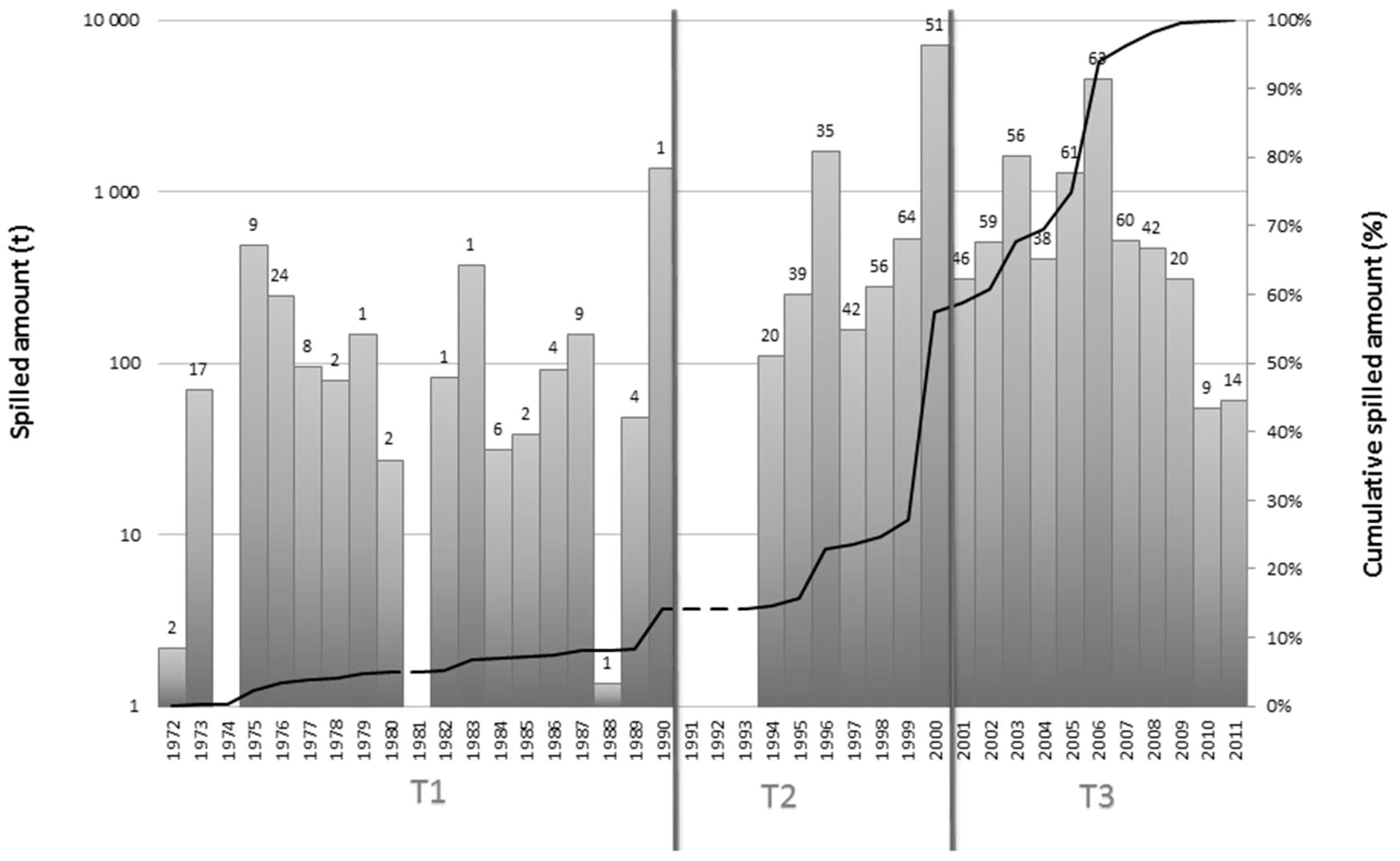
T1 (1972–1991): the foreign company Texaco and the National Petroleum Corporation (CEPE) were engaged in oil and gas activities. Over this period, the MEM estimated that 397.5 × 10⁶ t of crude oil were discharged to the environment [18].
T2 (1992–2001): State-owned Petro-Ecuador took over oil production. Data compilation on accidental oil spills was reinforced.
T3 (from 2001): period after the environmental decree taken for regulating oil activity (RAHOE).
Spatial gridding of disaggregated oil spills is useful for several purposes, including: pollution hotspot analysis, trajectory modelling, mapping of hazards and exposure, multiple-pollutant and risk assessments [19,20,21,22]. Only a few studies have attempted to make spatially explicit predictions of oil spills using kernel density estimation methods, with corrections based on data from surveillance efforts [23] and including human and other external factors associated with oil spill patterns [24]. Oil spill studies are typically performed in an offshore context, and only very few have looked at onshore events [2]. None of them included reliability analyses or validated models for the predicted patterns. Because institutional databases tend to be incomplete and heterogeneous, no study has ever attempted to use them to spatially estimate oil spill volumes in order to improve hazard or risk assessments.
The aim of the present study was to analyze oil spill patterns in the NEA. It focused on the T3 management period, in which monitoring was much improved compared to the previous periods [25]. Our aim was also to focus on recent contaminations to obtain up-to-date estimates of potential hazards. Surveys of local populations were used to determine spatial locations of oil spill sources and also how the contamination potential of oil spills is currently perceived [26], but these results require a more in-depth quantitative analysis. The present study builds a regional oil spill inventory and draws up spatially explicit oil spill maps. In parallel, the issue of incomplete and heterogeneous databases is addressed, so as to obtain estimated spill values in areas where data are incomplete. Finally, the reliability of our estimation procedure was analyzed using a cross-validation method, and the factors most likely to influence the quality of our estimates were assessed using simulated data.

2. Materials and Methods
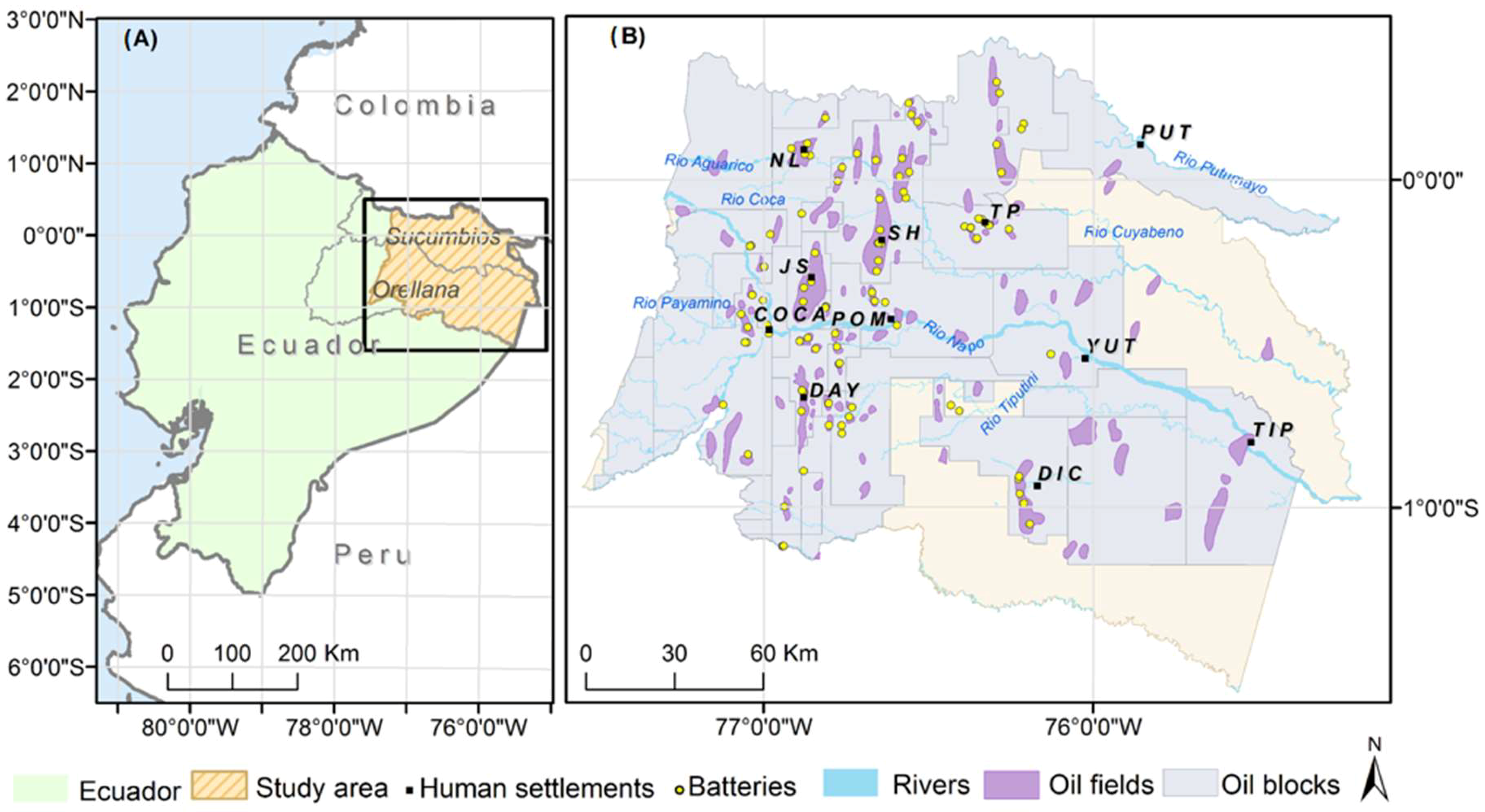
2.1. Study Area

The study was restricted to the provinces of Sucumbíos and Orellana in the NEA (~144–900 m a.s.l., Amazon lowlands), representing a surface area of 35,051 km2 (Figure 1A). The NEA is a biodiversity hotspot, including a large proportion of sensitive rainforest ecosystems. For instance, at least 210 mammals, 131 amphibians, 558 birds, and 3213 vascular plant species have been reported only in the Yasuni National Park [7,9]. Upstream oil and gas production infrastructures are found in this zone, and associated potentially polluting activities take place there (Figure 1B).

2.2. Data for Crude Oil Spills

In this study, oil pollution was quantitatively estimated and spatially allocated using GIS and institutional inventory databases, including the location of oil infrastructures and oil spills. Drilling platforms are positioned directly over producing oilfields, whereas oil separation batteries and refineries are located at Nueva Loja and Shushufindi (Figure 1). Distribution pipelines connect the oil wells to oil separation batteries, which are cylindrical or spherical vessels used to separate oil, gas and water from the total fluid stream produced by wells. Oil separation batteries are in turn joined to the main pipeline network so that products can be transported to oil separation batteries before being sent west, across the Andes Mountains to the coast for export. These data were obtained from PRAS or public online databases (Table 1). The data were disaggregated and categorized annually for the T3 period (more specifically for the 2001–2011 period, for which data were available).

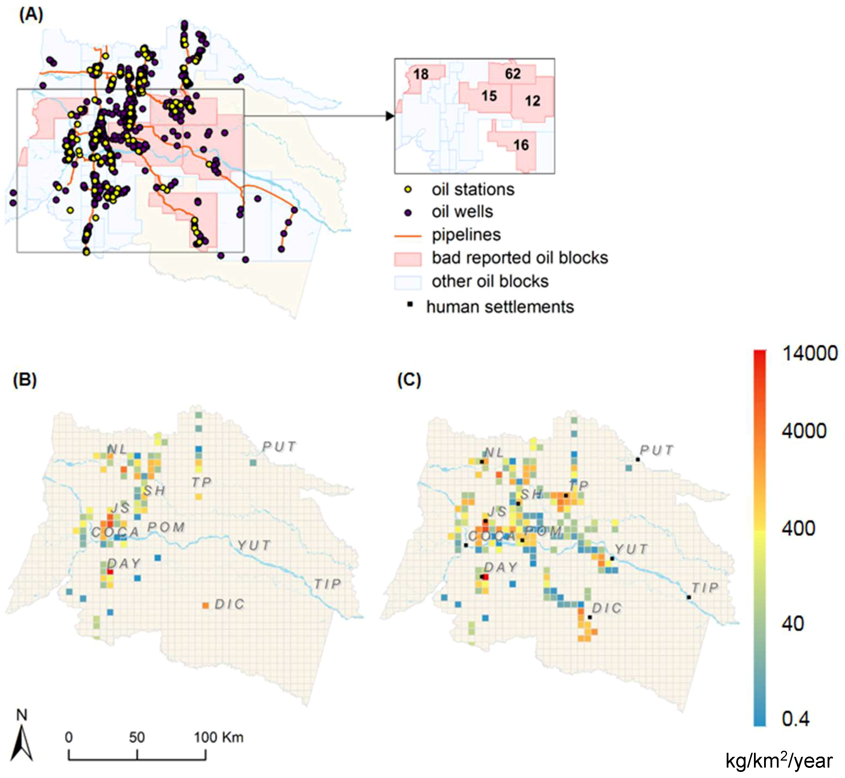
2.3. Accounting for Heterogeneity in Data Quality: Well- vs. Poorly-Documented Oil Blocks

In Ecuador, the central government organizes bidding rounds to award oil blocks to operators, who then each implement different management plans. This results in non-uniform environmental disclosures, meaning that oil spill reporting can vary greatly between oil blocks. There is indeed a strong contrast between some blocks with a high number of incidents recorded and others, sometimes comprising a large number of infrastructures, where few or no incidents have been reported.
It was therefore necessary to distinguish between well-documented and poorly-documented blocks. Assuming that incidents on a single infrastructure occur at a constant rate and are independent of one another, the number of incidents over a given time period can be described by the Poisson distribution [24,27]. The probability of n incidents occurring during the study period is therefore
P   ( n )   =   λ n   e   λ n !
where
n = 
number of oil spills on the block from 2001 to 2011.
λ = 
expected number of oil spills from 2001 to 2011 calculated based on the number of oil infrastructures on the block and the oil spill rate for all the oil blocks in the study area.
Parameter λ was estimated using oil well data; wells account for 70% of oil infrastructures and are therefore considered as representative of all the infrastructures in the area. Oil blocks were categorized as poorly-documented (i.e., the probability of observing such a low number of oil spills over the time period was highly unlikely) if P (n ≤ nobs.) < 0.05, and as well-documented otherwise.

2.4. Calculating the Oil Spill Rates to be Used for Estimations on Poorly-Documented Blocks

The oil spill rates for poorly-documented blocks were considered inaccurate and were therefore replaced by the rate found as described above, using data from well-documented blocks. Based on the raw data obtained from these blocks, the annual average spill volumes were calculated separately for three types of infrastructures: oil wells, oil separation batteries, and pipelines. These rates were expressed per infrastructure unit for oil wells and oil batteries and per kilometer for pipelines and were subsequently used to estimate spills within poorly-documented blocks, assuming a constant incident risk across the study area.
The possibility of using spatial information to improve the accuracy of this oil spill rate depending on infrastructure location (e.g., proximity to human settlements might entail greater surveillance efforts) was examined through a geostatistical approach. For this purpose, the Getis–Ord (Gi) statistic and Moran’s I index value were calculated. The Gi assesses the degree of clustering [28] and the Moran’s I index value made it possible to assess the spatial dependence of values, or autocorrelation. This index ranges from +1 to −1: positive values indicate clustering, negative values indicate dispersion and values close to 0, complete spatial randomness [29].

2.5. Oil Spill Mapping

In order to represent crude oil spills in a GIS environment, a grid with cells of 5 × 5 km was chosen to plot the spills and incorporate line and point infrastructure sources in the region. Spatial data processing was performed in ArcGIS®.
Two maps were created, one plotting actual oil spills from recorded events, a second taking into account heterogeneity in data quality and plotting estimated spills based on rates from well-documented blocks. This second map is a plausible spatial representation of oil spills.
Estimated spills were thus allocated to all infrastructures within the study area (excluding infrastructures that were not in production from 2001 to 2011). Estimated oil spill volumes at single point and line sources were added together within each grid cell to obtain total oil spill volumes per square kilometer and per year [2,19]. Values were mapped according to geometric intervals.

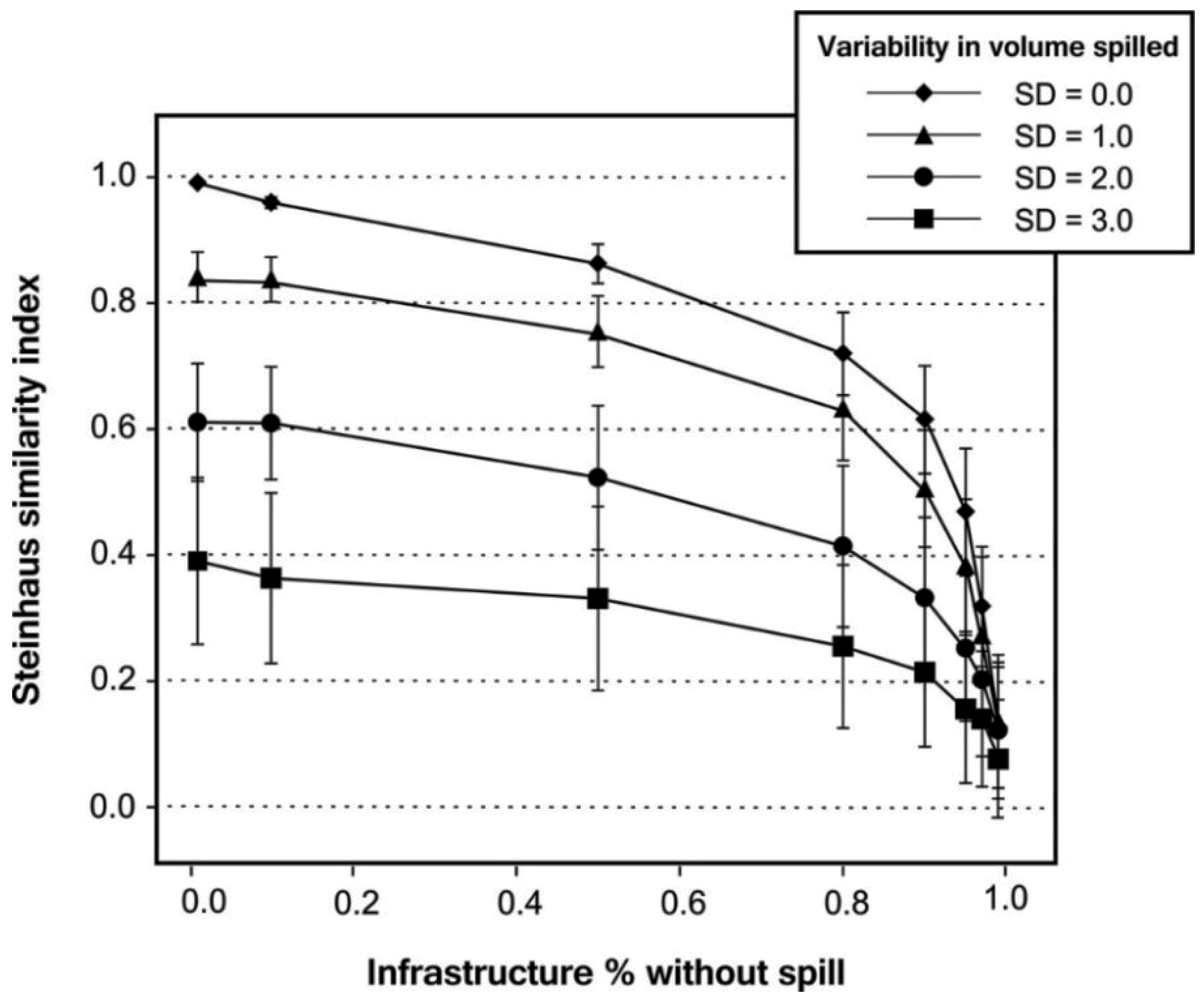
2.6. Validity of the Procedure to Estimate Oil Spills on Poorly-Documented Blocks

The reliability of the method used to estimate oil spills on poorly-documented blocks was assessed using a cross-validation procedure, drawing on data from well-documented blocks. This dataset was divided into two parts: the first would be used to compute spill factors for the various infrastructure types (i.e., the training subset), the second to estimate the oil spill volumes within each cell and to then compare these estimated values with those actually observed (i.e., the testing subset).
Similarity indices were used to compare estimated vs. observed values. For this purpose, two different metrics were used, both designed for quantitative data and ranging from 0 (extremely dissimilar samples) to 1 (identical samples). The first one, Gower’s coefficient [30], is symmetrical as it considers double zeros as a similarity (i.e., a negative match). The second one, the Steinhaus coefficient [31], is asymmetrical as it is not influenced by double zeros, and therefore gives greater emphasis to cells where oil infrastructures are located. In addition, the Pearson correlation coefficient was also calculated.
This procedure was repeated 1000 times, using a random allocation of cells either to training or test subsets. It was therefore possible to calculate average similarity coefficients and their standard deviations. To determine the significance of these similarity coefficients, a Monte Carlo procedure was performed, in which similarity coefficients were also calculated after observed and estimated spill volumes were randomly matched in order to generate a null distribution of the similarity/correlation coefficients (10,000 permutations computed).
Finally, to analyze to what extent the similarity coefficients were influenced by the variability in oil spill events, a simplified simulation-based approach was implemented, focused on oil wells. Using a uniform distribution to allocate oil spills to the wells, and a log-normal distribution to simulate the volumes spilled (which was the best choice with regard to the distribution of the real oil spills observed, whose volumes spanned four orders of magnitude [32]), various datasets were randomly generated including different percentages of wells where no event had been reported over the given time period and different standard deviations of volumes spilled in each event. The σ parameter of the log-normal distribution for spill volumes was set between 0.0 and 3.0 in the various simulations. The µ parameter was set at 3.5 in simulations where spills had occurred on all the wells, and this value was changed accordingly in subsequent simulations to take into account the increase in the percentage of oil wells where there had been no spill.

3. Results

3.1. Oil Spills: Temporal and Spatial Patterns

Historical data indicate that oil spills occurred before 2001 and represented a total spill volume of 20,386 t. From 2001 to 2011, 464 accidental oil spills accounting for a total amount of 10,000.2 t were identified and documented by the PRAS of the Ministry of the Environment of Ecuador. 41.3% of the total volume of oil spilled was reported to have occurred in the T3 period, the focus of our study. The number of oil spills per year decreased from 2007 to 2011 for all infrastructures. Figure 2 presents the overall annual number of incidents and spill volumes.
Table 2 summarizes the spatial variations and average values in the number of accidental oil spills and spill volumes from 2001 to 2011. The different blocks give a total spill volume of 10,000.2 t, associated either with oil wells/platforms (6971.7 t, n = 339), oil separation batteries (2555.7 t, n = 107), or pipeline infrastructures (472.9 t, n = 7). Oil wells/platforms therefore contribute to ca. 70% of oil spill volumes, while the 605 km of pipelines recorded account for less than 5%. Four oil blocks account for >90% of the spill volumes, namely Auca, Sacha, Libertador, and Lago Agrio.
Figure 3A shows the locations of point sources, i.e., oil wells (n = 668) and oil and gas batteries (n = 108), and line sources: 1596.37 km of recorded pipeline. Most of the infrastructures are located in the northwest of the country, in the cities of Nueva Loja, Joya de Los Sachas, and Shushufindi.
No spatial pattern could be identified with the metrics used (neither at block nor regional scales), neither in terms of spill volumes (Gi = 0.0028, Z = −0.66, P = 0.51; I Moran’s index = 0.006, Z = 0.56, P = 0.57) nor incident occurrences (Gi = 0.0038, Z = −0.14, P = 0.89; I Moran’s index = −0.024, Z = −0.84, P = 0.39), and no infrastructure attribute (except for typology, i.e., well, battery or pipeline) could be significantly correlated with oil spill rates. The best option for estimating oil spill volumes on poorly-documented oil blocks was therefore to use average constant allocation drawing on spill rates from properly-documented blocks.
The following two maps: (1) spills actually recorded (Figure 3B) and (2) spatially-allocated estimates (for poorly-documented oil blocks) associated with recorded spills (for well-documented blocks) (Figure 3C) were used to investigate oil spill patterns. These maps show different levels of spills, mainly concentrated in the four oil blocks already mentioned (Table 2 and Figure 3B), and highlight spill hotspots (Figure 3B). Spatial allocation of oil spills to poorly-documented oil blocks naturally resulted in an increase in total spill volumes.
Our final spatial distribution map shows that a hypothetical total of 15,481.5 t of oil was spilled in the NEA i.e., a 54.8% increase compared to the recorded total (Table 2). The variations in spills on the harmonized map for each type of infrastructure are: 4494 t for oil wells/platforms (82.0% of the total increase), 835 t for oil separation batteries (15.2%), and 153 t for pipelines (2.8%). The cities of Tarapoa, Yuturi, Dícaro, and Puerto Francisco de Orellana in the east all displayed larger oil spill volumes than in the original dataset (Figure 3C).

3.2. Reliability of the Procedure Used to Estimate Missing Data

Although assessing the validity of our approach on presumably poorly-documented oil blocks was impossible due to the age of the oil spills, difficulties in accessing the fields, and the absence of any further data, it was however feasible to evaluate the reliability of the method implemented using data from properly-documented blocks. Similarity metrics between estimated and observed spill volumes across the 942 grid-cells from well-documented blocks amounted to 0.97, 0.58, and 0.32 for Gower’s coefficient, the Pearson correlation coefficient, and the Steinhaus index respectively.
The high average value obtained with Gower’s coefficient was related to the large number of null values in the dataset and to the symmetrical nature of this index, giving some weight to double-zeros. Such a high Gower index value is actually very likely to be obtained only by chance, as shown by the Monte-Carlo procedure (10,000 permutations, p = 0.84). In contrast, the Steinhaus index does not take double-zeros into account in similarity computations, and therefore focuses on the grid-cells where oil infrastructures are located. Although not very high, its value is significant according to the results of the Monte-Carlo procedure (10,000 permutations, p = 0.0016), as is the value obtained with the Pearson correlation coefficient (10,000 permutations, p = 0.0087).
By using an exploratory approach on simulated data, we were able to investigate to what extent our predictive ability would be affected by the sources of spatiotemporal variability in oil spill patterns. Figure 4 shows that the similarity between observed and estimated spills obtained with the Steinhaus index is high (i.e., above 0.8) when both incident occurrence and spill volumes are highly predictable. In contrast, even if spill volumes remain predictable, this similarity drops when the stochasticity of events increases.

4. Discussion

4.1. Uncertainties and Data Quality

4.1.1. Data Reporting

In the NEA, oil spills decreased in later years, in line with global trends [33]. In keeping with other studies [2,23,24], this work suggests there are primarily two reasons for this: (1) activities are better managed and there is a general tendency for spills to decrease; and (2) surveillance efforts might be less consistent than in previous years because of reduced data disclosure. The maps provided in the present study are the most accurate representations of the spatial distribution of oil spills according to available data. In this respect, the PRAS dataset is a thorough compilation of environmental assessments performed by several local government agencies. The multiplicity of data sources is not an obstacle to running a comprehensive analysis of oil spill patterns, provided certain quality requirements are fulfilled [2]. In the present study, the uncertainties related to using oil spills at specific infrastructure points are acknowledged and require caution when using these data. However, in a 5 × 5 km2 grid, the effects of location errors are presumably less significant.

4.1.2. Spill Estimates

Estimating the quantity of hydrocarbons accidentally discharged to the environment remains a difficult task and requires good incident tracking/reporting. Data records are often not exhaustive because industry operators do not necessarily disclose information, and data disclosure can vary depending on the operator and their respective management plans [16,34]. In this respect, it should be noted that most of the oil spills recorded occurred on blocks managed by the national state company. ‘Poorly-documented’ oil blocks are categorized as such based on the assumption that data are incomplete, following statistical analysis. However, the statistically significant lower occurrence of events on these blocks could also be related to more efficient management by oil operators. These different scenarios could generate alternative results, and it could be assumed that the proper distribution of oil spills lies somewhere between official and computed patterns (Figure 3B,C).

4.2. Accuracy of Oil Spill Estimations

Incidents can occur because of infrastructure corrosion, human errors during oil production and transport, politically-motivated attacks, natural disasters, and so on [35,36]. The causes of oil spills have been documented in the PRAS database and could have helped to improve the oil spill predictions. For instance, one hypothesis is that greater efforts are put into surveillance in the vicinity of settlements, leading to improved incident reporting, or that incident rates are higher in some areas than in others (zones subject to flooding or seismic activity). However, this was not supported by the data and, more generally, exploratory spatial analyses of oil spills were not conclusive as no clustering or autocorrelation was found in spill rates or volumes. The only information that proved useful for refining predictions was the type of infrastructure (i.e., wells, batteries, pipelines), which enabled us to estimate different spill rates. As a result, our ability to predict oil spills within the study area is relatively limited, as shown by the cross-validation performed on presumably properly-documented oil blocks: when no weight was given to double-zeros (often corresponding to grid cells devoid of oil infrastructures), ca. only 30% of spatial variations in oil spill volumes could be predicted.
This value was much improved (reaching 97%) with Gower’s coefficient, giving some weight to the cells where there is no oil infrastructure. This highlights the importance of choosing the right metric to assess similarity. Although the Steinhaus index is better suited in the present case to assess the quality of our estimation method, this may be relevant to use Gower’s coefficient for assessing the reliability of the contamination patterns predicted at the regional scale, without excluding the trivial situations corresponding to the areas where there is no oil infrastructure and thus no oil spill.
The analysis of simulated situations has shown that the ability to predict oil spills is strongly dependent on unexplained variabilities in incident rates and spill volumes. In other words, a lower variability in spill patterns logically improves predictions. Low variability can be observed in other contexts, for instance when spills are mostly due to continuous infrastructure leaks [37]. This also implies that any data-mining method allowing to reduce the part of residual variability in oil spill patterns will improve predictions. Beyond the methods used in the present study, other approaches such as machine-learning algorithms could potentially help to improve the estimation accuracy of spill factors, provided features of oil and gas infrastructures and/or spatial data are available and offer sufficient information about event probability or severity [38].

4.3. Spatial Distribution of Spills and Hazard Potential

Pollution hotspots could be identified from the two oil spill maps (Figure 3B,C). Joya de Los Sachas displays the highest level of pollution, but other sites also exhibit high levels of spills such as Yuturi, Dayuma, and the area from Shushufindi to Nueva Loja. Owing to the spill volumes allocated to poorly-documented blocks, Dícaro and Tarapoa appear as potential areas of concern too. Ongoing research aims to combine maps depicting the impacts to the different environmental compartments (atmosphere, pedosphere, and hydrosphere) and classify them by pollutants (e.g., black carbon, total hydrocarbons, heavy metals) from different sources (accidental oil spills, mud drilling pits, and gas flares).
Achieving the target of zero harmful discharges is a real challenge. However, our data analysis does differentiate sites where oil spills exceed hazard severity thresholds and where the potential economic, health, and environmental losses are the highest. Severe oil spills are better defined when one or more of the following criteria are met, including the amount spilled, remediation costs, the impacted area, and the environmental damage sustained in an single event [39]. Data in this study offered the opportunity to directly investigate the first criterion. For instance, an individual spill of 10,000 t is generally considered as a severity threshold; however, other standard international thresholds give lower amounts (34–136 t) [2] comparable to spill volumes in the present study (Table 3). These hazard thresholds are exceeded in several locations across the NEA, but are not highlighted by our estimations and spatial maps due to the grid resolution and time scale used. Other studies, however, suggest chronic pollution from oil spills in the NEA [23,40], and the mapping of total pollution over a longer period (2001–2011) might better estimate hazard-prone areas in the case of low-volume but recurrent spill events.
Oil spills by infrastructure type are in concordance with worldwide historical reports [2,33]. The most severe spills originated from tankers during offshore activities. This source aside, 8.7% of the spills recorded worldwide were due to pipelines and 29.3% to oil wells/platforms. Similarly, data recorded in the NEA gave these sources as responsible for 4.7% and 95.3% of spills, respectively. This goes against the common belief that oil spills are essentially due to pipelines [1].

4.4. Potential Economic, Health, and Environmental Losses

A study performed by the International Oil Pollution Compensation Fund (IOPCF), founded on a historical oil spill dataset, derived a conversion factor of USD 51,437 per ton of oil spilled, based on costs associated with environmental damage; clean-up; and losses in the fishery, tourism, and farming sectors [41]. When this factor is applied to our case study, a sum of USD 514.4 million is obtained for the whole period considered (2001–2011), i.e., USD 46.8 million/year (USD 72.4 million/year if the predicted spill volumes in poorly-documented blocks are taken into account). This is an early reference cost as until now the factor was generally applied to datasets from offshore oil spills; further site-specific analyses need to be conducted in this sensitive area.
In the NEA, studies have revealed the acute toxicity of drinking water and sediment, increasing the vulnerability of freshwater ecosystems [42] and causing human health issues, ranging from dizziness to cancer [36,39]. Future studies should deepen understanding of other hazard sources (i.e., waste pits) at local and regional scales. Hazard maps could improve decision-making, when combined with vulnerability maps (e.g., groundwater, biodiversity values, etc.). Previous studies have assessed the risk of oil concessions merely by overlaying hazards with maps of vulnerable assets at larger scales, with a lower spatial resolution, and greater surface areas than the ones in this study [9,10,43]. This study is therefore more comprehensive and offers the potential for integrating spatio-temporal patterns of contamination; this represents a first step towards spill maps that could be used as input to model contaminant dispersion and trajectory, or to improve risk assessments at finer scales and spatial resolutions when associated with vulnerability maps.

5. Conclusions

This study presents a ‘bottom-up approach’ to processing and visually representing datasets specific to upstream oil and gas production activities (i.e., type of infrastructure) in gridded form. In addition, the estimation of spills and the subsequent harmonized spatial distribution of pollutants in the NEA are of great importance for this sensitive area, as they potentially provide information about the hazards posed by these activities. This forms a set of regional and local multiple-source spill data combining the latest available local information with spatio-temporal allocation. Overall, the sum of incidents having occurred at oil separation batteries and oil wells/platforms during the T3 management period contradicts the common belief that they represent only a small share of spill sources compared to pipeline networks. The willingness of institutions and operators to disclose data is the key. Data disclosure could help improve evaluation of pollutant releases for more effective decision-making in land use planning to improve health, economic, and environmental conditions. Finally, spill maps represent the total potential oil spill hazard, which could be useful for future risk assessments in a context of scarce reliable data to predict oil spills.

Author Contributions

Conceptualization, A.E., M.S., and J.D.-C.; Methodology, A.E., M.S., C.L., and J.D.-C.; Software, J.D.-C., M.L., and A.E; Validation, A.E. and C.L.; Formal analysis, J.D.-C., M.L., and A.E; Investigation, M.L. and J.D.-C.; Resources, A.E. and M.S.; Data curation, A.E.; Writing—original draft preparation, J.D.-C.; Writing—review and editing, J.D.-C., M.S., and A.E.; Visualization, J.D.-C.; Supervision, A.E.; Project administration, M.S. and J.D.-C.; Funding acquisition, J.D.-C. and A.E.

Funding

This research was funded by the Ecuadorian National Secretary of Higher Education, Science and Technology (SENESCYT) for the financial support provided and the ANR-MONOIL Project N ANR-13-SENV-0003-01.

Acknowledgments

The authors would like to thank local officials from the PRAS, who provided the data and valuable advice and information to improve the quality of this paper. They gratefully acknowledge Elaine Hannan for correcting the English text.

Conflicts of Interest

The authors declare no conflict of interest. The funders had no role in the design of the study; in the collection, analyses, or interpretation of data; in the writing of the manuscript, or in the decision to publish the results.

References

  1. Jernelöv, A. The Threats from Oil Spills: Now, Then, and in the Future. Ambio 2010, 39, 353–366. [Google Scholar] [CrossRef] [Green Version]
  2. Burgherr, P. In-depth analysis of accidental oil spills from tankers in the context of global spill trends from all sources. J. Hazard. Mater. 2007, 140, 245–256. [Google Scholar] [CrossRef]
  3. Chang, S.E.; Stone, J.; Demes, K.; Piscitelli, M. Consequences of oil spills: A review and framework for informing planning. Ecol. Soc. 2014, 19, 26. [Google Scholar] [CrossRef]
  4. Wernersson, A.-S. Aquatic ecotoxicity due to oil pollution in the Ecuadorian Amazon. Aquat. Ecosyst. Health Manag. 2004, 7, 127–136. [Google Scholar] [CrossRef]
  5. Bondur, V.G. Aerospace methods and technologies for monitoring oil and gas areas and facilities. Izv. Atmos. Ocean. Phys. 2011, 47, 1007–1018. [Google Scholar] [CrossRef]
  6. Myers, N.; Mittermeier, R.A.; Mittermeier, C.G.; da Fonseca, G.A.B.; Kent, J. Biodiversity hotspots for conservation priorities. Nature 2000, 403, 853–858. [Google Scholar] [CrossRef]
  7. Bass, M.S.; Finer, M.; Jenkins, C.N.; Kreft, H.; Cisneros-Heredia, D.F.; McCracken, S.F.; Pitman, N.C.A.; English, P.H.; Swing, K.; Villa, G.; et al. Global conservation significance of Ecuador’s Yasuní National Park. PLoS ONE 2010, 5, e8767. [Google Scholar] [CrossRef]
  8. Larrea, C. Hacia una Historia Ecológica del Ecuador: Propuestas para el Debate; Biblioteca General de Cultura: Quito, Ecuador, 2006. [Google Scholar]
  9. Finer, M.; Jenkins, C.N.; Pimm, S.L.; Keane, B.; Ross, C. Oil and Gas Projects in the Western Amazon: Threats to Wilderness, Biodiversity, and Indigenous Peoples. PLoS ONE 2008, 3, e2932. [Google Scholar] [CrossRef]
  10. Baynard, C.W.; Ellis, J.M.; Davis, H. Roads, petroleum and accessibility: The case of eastern Ecuador. GeoJournal 2013, 78, 675–695. [Google Scholar] [CrossRef]
  11. Butt, N.; Beyer, H.L.; Bennett, J.R.; Biggs, D.; Maggini, R.; Mills, M.; Renwick, A.R.; Seabrook, L.M.; Possingham, H.P. Biodiversity risks from fossil fuel extraction. Science 2013, 342, 425–426. [Google Scholar] [CrossRef]
  12. Waldner, C.L.; Ribble, C.S.; Janzen, E.D.; Campbell, J.R. Associations between oil- and gas-well sites, processing facilities, flaring, and beef cattle reproduction and calf mortality in western Canada. Prev. Vet. Med. 2001, 50, 1–17. [Google Scholar] [CrossRef]
  13. Sebastián, M.S.; Armstrong, B.; Córdoba, J.A.; Stephens, C. Exposures and Cancer Incidence near Oil Fields in the Amazon Basin of Ecuador. Occup. Environ. Med. 2001, 58, 517–522. [Google Scholar] [CrossRef]
  14. San Sebastián, M.; Hurtig, A.K. Oil development and health in the Amazon basin of Ecuador: The popular epidemiology process. Soc. Sci. Med. 2005, 60, 799–807. [Google Scholar] [CrossRef]
  15. Boxall, P.C.; Chan, W.H.; Mcmillan, M.L. The impact of oil and natural gas facilities on rural residential property values: A spatial hedonic analysis. Resour. Energy Econ. 2005, 27, 248–269. [Google Scholar] [CrossRef]
  16. Buccina, S.; Chene, D.; Gramlich, J. Accounting for the environmental impacts of Texaco’s operations in Ecuador: Chevron’s contingent environmental liability disclosures. Account. Forum 2013, 37, 110–123. [Google Scholar] [CrossRef]
  17. Juteau, G.; Becerra, S.; Maurice, L. Environment, oil and political vulnerability in the Ecuadorian Amazon: Towards new forms of energy governance? Am. Lat. Hoy 2014, 67, 119–137. [Google Scholar]
  18. Amazon Defense Front. Breve Historia de las Operaciones de Texaco en el Oriente Ecuatoriano 1964–1990. Unpublished Work. 2008. [Google Scholar]
  19. Andreo, B.; Goldscheider, N.; Vadillo, I.; Vías, J.M.; Neukum, C.; Sinreich, M.; Jiménez, P.; Brechenmacher, J.; Carrasco, F.; Hötzl, H.; et al. Karst groundwater protection: First application of a Pan-European Approach to vulnerability, hazard and risk mapping in the Sierra de Líbar (Southern Spain). Sci. Total Environ. 2006, 357, 54–73. [Google Scholar] [CrossRef]
  20. Guttikunda, S.K.; Calori, G. A GIS based emissions inventory at 1 km × 1 km spatial resolution for air pollution analysis in Delhi, India. Atmos. Environ. 2013, 67, 101–111. [Google Scholar] [CrossRef]
  21. Lahr, J.; Kooistra, L. Environmental risk mapping of pollutants: State of the art and communication aspects. Sci. Total Environ. 2010, 408, 3899–3907. [Google Scholar] [CrossRef]
  22. Lahr, J.; Münier, B.; De Lange, H.J.; Faber, J.F.; Sørensen, P.B. Wildlife vulnerability and risk maps for combined pollutants. Sci. Total Environ. 2010, 408, 3891–3898. [Google Scholar] [CrossRef] [Green Version]
  23. Serra-Sogas, N.; O’Hara, P.D.; Canessa, R.; Keller, P.; Pelot, R. Visualization of spatial patterns and temporal trends for aerial surveillance of illegal oil discharges in western Canadian marine waters. Mar. Pollut. Bull. 2008, 56, 825–833. [Google Scholar] [CrossRef]
  24. Bertazzon, S.; O’Hara, P.D.; Barrett, O.; Serra-Sogas, N. Geospatial analysis of oil discharges observed by the National Aerial Surveillance Program in the Canadian Pacific Ocean. Appl. Geogr. 2014, 52, 78–89. [Google Scholar] [CrossRef]
  25. SENPLADES. Atlas de las Desigualdades Socioeconómicas del Ecuador; Larrea, C., Camacho, G., Eds.; TRAMA: Quito, Ecuador, 2013; ISBN 9789942074782. [Google Scholar]
  26. Maestripieri, N.; Saqalli, M. Assessing health risk using regional mappings based on local perceptions: A comparative study of three different hazards. Hum. Ecol. Risk Assess. 2016, 22, 721–735. [Google Scholar] [CrossRef]
  27. Smith, R.; Slack, J.; Wyant, T.; Lanfear, K. The Oilspill Risk Analysis Model of the U.S. Geological Survey; US Geological Survey: Washington, DC, USA, 1982.
  28. Getis, A.; Ord, J.K. The Analysis of Spatial Association by Use of Distance Statistics. Geogr. Anal. 1992, 24, 189–206. [Google Scholar] [CrossRef]
  29. Meng, Q. Spatial analysis of environment and population at risk of natural gas fracking in the state of Pennsylvania, USA. Sci. Total Environ. 2015, 515–516, 198–206. [Google Scholar] [CrossRef] [PubMed]
  30. Gower, J.C. A General Coefficient of Similarity and Some of Its Properties. Biometrics 1971, 27, 857–871. [Google Scholar] [CrossRef]
  31. Legendre, P.; Legendre, L. Numerical Ecology, 2nd ed.; Elsevier B.V.: Amsterdam, The Netherlands, 1998. [Google Scholar]
  32. Limpert, E.; Stahel, W.A.; Abbt, M. Log-normal Distributions across the Sciences: Keys and Clues. Bioscience 2001, 51, 341–352. [Google Scholar] [CrossRef]
  33. Schmidt Etkin, D. Analysis of Oil Spill Trends in the United States and Worldwide. 2001. Available online: http://www.environmental-research.com/publications/pdf/spill_statistics/paper4.pdf (accessed on 15 August 2017).
  34. Schweitzer, L. Accident frequencies in environmental justice assessment and land use studies. J. Hazard. Mater. 2008, 156, 44–50. [Google Scholar] [CrossRef]
  35. Darbra, R.M.; Palacios, A.; Casal, J. Domino effect in chemical accidents: Main features and accident sequences. J. Hazard. Mater. 2010, 183, 565–573. [Google Scholar] [CrossRef]
  36. Burgherr, P.; Eckle, P.; Hirschberg, S. Comparative assessment of severe accident risks in the coal, oil and natural gas chains. Reliab. Eng. Syst. Saf. 2012, 105, 97–103. [Google Scholar] [CrossRef]
  37. McKain, K.; Down, A.; Raciti, S.M.; Budney, J.; Hutyra, L.R.; Floerchinger, C.; Herndon, S.C.; Nehrkorn, T.; Zahniser, M.S.; Jackson, R.B.; et al. Methane emissions from natural gas infrastructure and use in the urban region of Boston, Massachusetts. Proc. Natl. Acad. Sci. USA 2015, 112, 1941–1946. [Google Scholar] [CrossRef] [PubMed] [Green Version]
  38. Arellano, P.; Tansey, K.; Balzter, H.; Boyd, D.S. Detecting the effects of hydrocarbon pollution in the Amazon forest using hyperspectral satellite images. Environ. Pollut. 2015, 205, 225–239. [Google Scholar] [CrossRef] [PubMed]
  39. Burgherr, P.; Hirschberg, S. Comparative risk assessment of severe accidents in the energy sector. Energy Policy 2014, 74, S45–S56. [Google Scholar] [CrossRef]
  40. Bissardon, P.; Becerra, S.; Maurice, L. Le risque sanitaire lié aux activités pétrolières en Amazonie équatorienne: Des alertes aux décisions. Environ. Risque Sante 2013, 12, 338–344. [Google Scholar] [CrossRef]
  41. Kontovas, C.A.; Psaraftis, H.N.; Ventikos, N.P. An empirical analysis of IOPCF oil spill cost data. Mar. Pollut. Bull. 2010, 60, 1455–1466. [Google Scholar] [CrossRef]
  42. Castello, L.; Mcgrath, D.G.; Hess, L.L.; Coe, M.T.; Lefebvre, P.A.; Petry, P.; Macedo, M.N.; Ren, V.F.; Arantes, C.C. The vulnerability of Amazon freshwater ecosystems. Conserv. Lett. 2013, 217–229. [Google Scholar] [CrossRef]
  43. Cuba, N.; Bebbington, A.; Rogan, J.; Millones, M. Extractive industries, livelihoods and natural resource competition: Mapping overlapping claims in Peru and Ghana. Appl. Geogr. 2014, 54, 250–261. [Google Scholar] [CrossRef]
Figure 1. (A) The NEA in Ecuador; (B) study area within the two NEA provinces of Sucumbíos and Orellana including oil fields and oil separation batteries. The names of the human settlements represented are abbreviated: DAY = Dayuma; NL = Nueva Loja (aka. Lago Agrio); SH = Shushufindi; TP = Tarapoa; PUT = Putumayo; COCA = Puerto Francisco de Orellana; JS = Joya de Los Sachas; YUT = Yuturi; DI = Dícaro; TP = Tiputini.
Sustainability 10 04719 g001
Figure 2. Number of accidental oil spills per year (individual values shown at the top of each bar) and the corresponding cumulative percentages relative to the total spill volume over the whole period. No datum was recorded from 1991 to 1993 (departure of Texaco).
Sustainability 10 04719 g002
Figure 3. Spatial variations in oil spills during the T3 management period (2001–2011). (A) Map of the NEA showing the main oil infrastructures with well-documented (blue) and poorly-documented (red) oil blocks. (B) Originally recorded spills. (C) Harmonized map plotting data from (B) for well-documented oil blocks and average constant allocation to poorly-documented oil blocks.
Sustainability 10 04719 g003
Figure 4. Variations of the Steinhaus index assessing the similarity between observed and estimated oil spill volumes across a simulated area of 23,550 km2, as a function of different sources of heterogeneity. This highlights the influence of variabilities in incident rates (i.e., spills evenly distributed across infrastructures vs. concentrated among a small proportion of infrastructures) and in the volume of oil spilled per incident.
Sustainability 10 04719 g004
Table 1. Databases used in this study.
GIS DataDescriptionSources
Oil blocks, oilfieldsPolygons, 1:250,000National Board of Hydrocarbons (2014)
Petro Ecuador (2013)
Oil wells, platforms, refineries, oil separation batteriesPointsPRAS (1972–2014)
Oil spillsPointsPRAS (1972–2014)
PipelinesLinesSENPLADES (2009)
Inventories
Oil spillsHistorical dataPRAS (2014) and local governments
Table 2. Total and average values on original oil spill data. A total of 13 oil blocks are located within the study area and, considering all the infrastructures, only 4 of the 13 oil blocks present greater volumes. The subtotals are the results from a single oil block. Oil blocks by abbreviation and geographical location are shown as follows: AU = Auca, LA = Lago Agrio which are located in Pacayacu parish, LT = Libertador in Shushufindi, SC = Sacha in Joya de Los Sachas.
Oil Spill OccurrencesOil Spill Volumes
Total (n)Average (n/year)Total (t)Average (t/year)Share (%)
on oil blocks (N = 13)block 61 (AU)767 ± 5.824054.50368.59 (±1119.09)40.54
block 60 (SC)989 ± 7.82801.56254.68 (±324.87)28.01
block 57 (LT)15414 ± 7.51792.13162.92 (±159.80)17.92
block 56 (LA)535 ± 3.6368.7833.52 (±47.23)3.69
sub-total38134.6 ± 7.89016.97819.73 (±1170.14)90.17
on single infrastructureWells33930.82 ± 0.196971.66633.79 (±1149)69.71
Pipeline70.6472.8842.98 (±55.4)4.73
Oil separation batteries11810.7 ± 0.622555.7232.33 (±327.69)25.56
Total46442.210,000.23909.11 (±1219.46)100.00
Table 3. Number of emission events exceeding international severity thresholds over the period 2003–2012 in human settlements. The international standards selected are: The Environmental Technology Centre (ETC) and the Environmental Research Consulting (ERC). YUT, POM, and TP are in poorly-documented blocks, meaning the number of events might be higher.
LocationAbbr.ETC (136 t)ERC (34 t)
COCACOCA-2
DayumaDAY13
DicaroDIC11
Joya de los SachasJS821
Nueva LojaNL210
PompeyaPOM--
PutumayoPUT-1
ShushufindiSH-6
TarapoaTP-1
Yasuni-ITTTIP--
YuturiYUT--
Number 1245

