
Assessing the Impact of (Self)-Quarantine through a Basic Model of Infectious Disease Dynamics

Abstract
:1. Introduction
- The impact of asymptomatic infectious individuals on disease dynamics.
- The impact of (self)-quarantine on disease dynamics.
2. Materials and Methods
- We introduce a compartment for the asymptomatic infectious individuals.
- We model the effect of (self)-quarantine via the introduction of a new nonlinear (sublinear to be precise) transmission term.
- S—susceptible;
- E—exposed;
- A—asymptomatic infectious;
- I—symptomatic infectious;
- R—recovered/removed.
- Newly infected individuals all enter the exposed compartment first due to a latency period. It is clear from the studies that, for COVID-19, there is a significant incubation period of approximately days; see [18].
- Exposed individuals spend on average in the E compartment time units (where, e.g., for COVID-19 days, according to [18]), after which a proportion: of them becomes symptomatic infectious, while the remaining individuals become asymptomatic infectious.
- Both asymptomatic and symptomatic individuals may pass on the disease, but naturally (as is the case for all influenza-like diseases, spread mainly by droplets, e.g., COVID-19) the transmission rate is significantly higher for symptomatic individuals: , when compared to the transmission rate for asymptomatic infected individuals: ; that is ; still asymptomatic infected individuals may also pass on the disease (for example via very close contact).
- We take into account the effect of (self)-quarantine; that is, we assume that at any given time a subset of the symptomatic infected individuals (self)-quarantine (this is supported by reports, e.g., during the COVID-19 pandemic, see, e.g., [19,20]). We use a power law to model this, instead of using, for example, a fixed proportion, as it is known that (online) human interaction activity will impact adherence rates, and such activity can be often approximated by power laws (see, e.g., [21,22]). Moreover, it may be natural to assume that the impact of quarantine will be more significant for relatively higher infectious population densities. Thus, in combination with the classic mass action assumption, we propose to use an infection term of the following form:Note that, for smaller values of , the transmission (for example contact) between susceptibles and symptomatic infectious individuals is reduced. In particular, would correspond to a complete quarantine of the symptomatic infectious population.
- We do not incorporate population dynamics since we want to focus on the disease dynamics over a short period of time here (that is, for COVID-19, a 4-month period during March–July 2020). Moreover, we do not explicitly incorporate disease-induced mortality into our model, although it can be understood that deceased people have entered the removed compartment.

3. Results
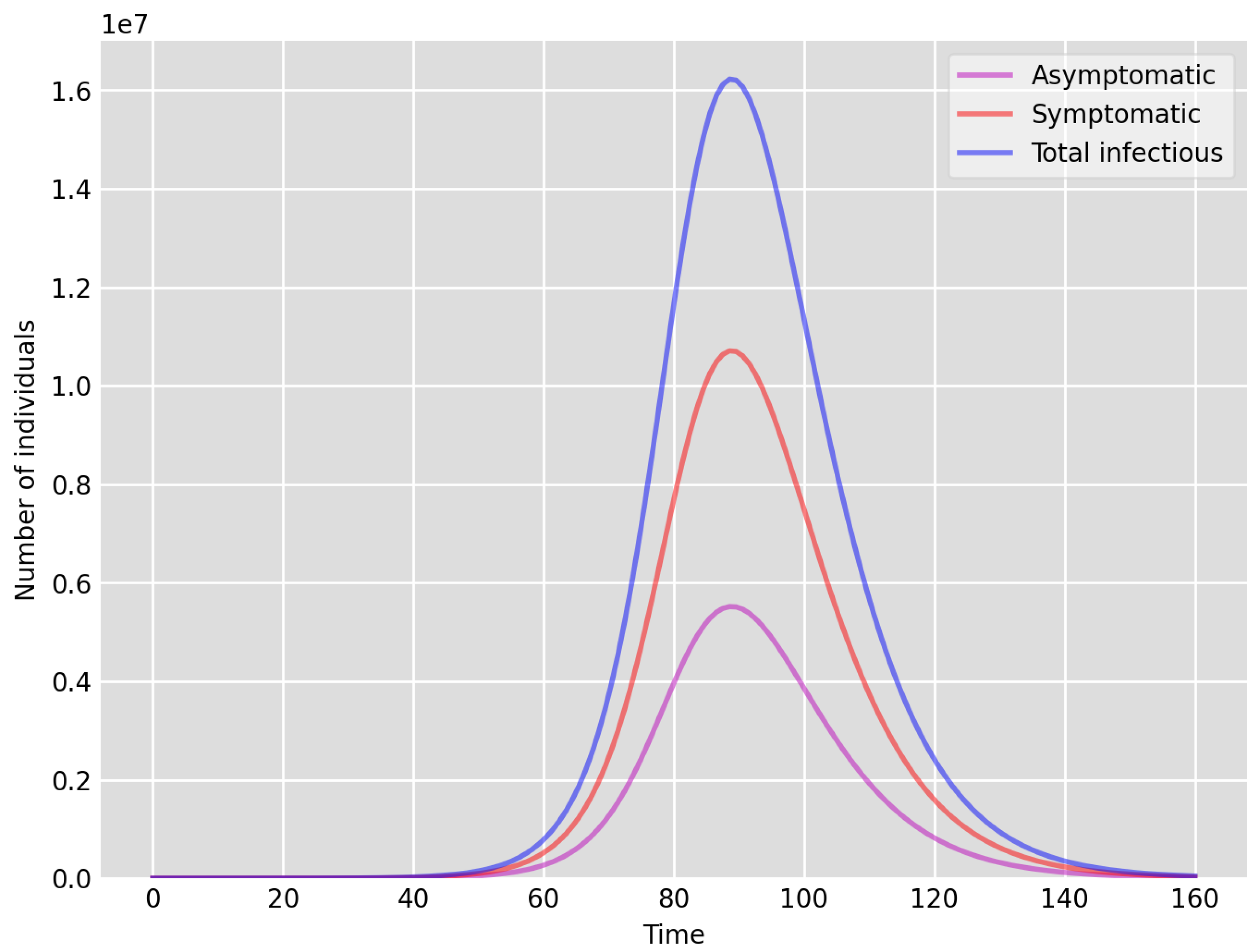
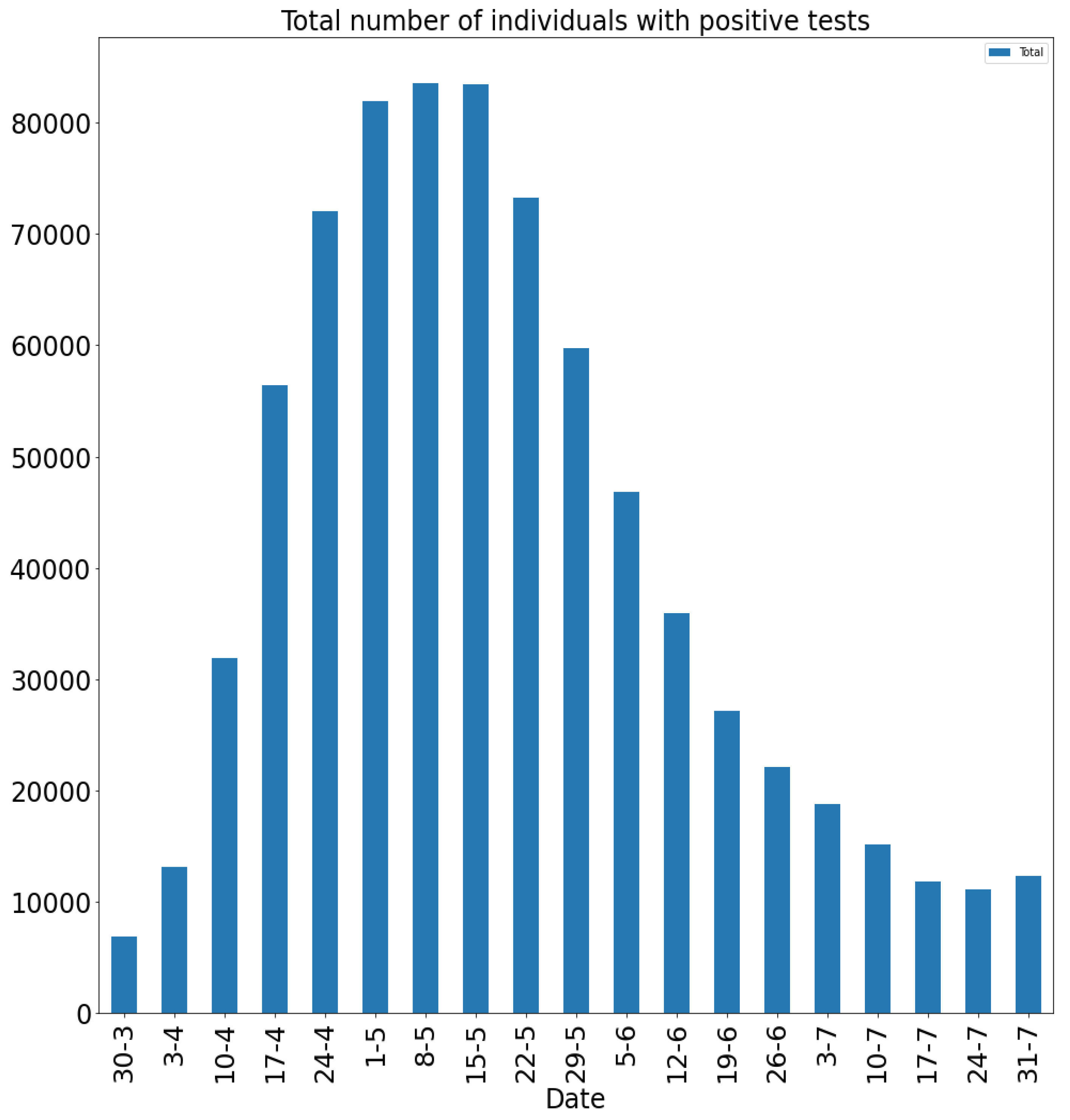
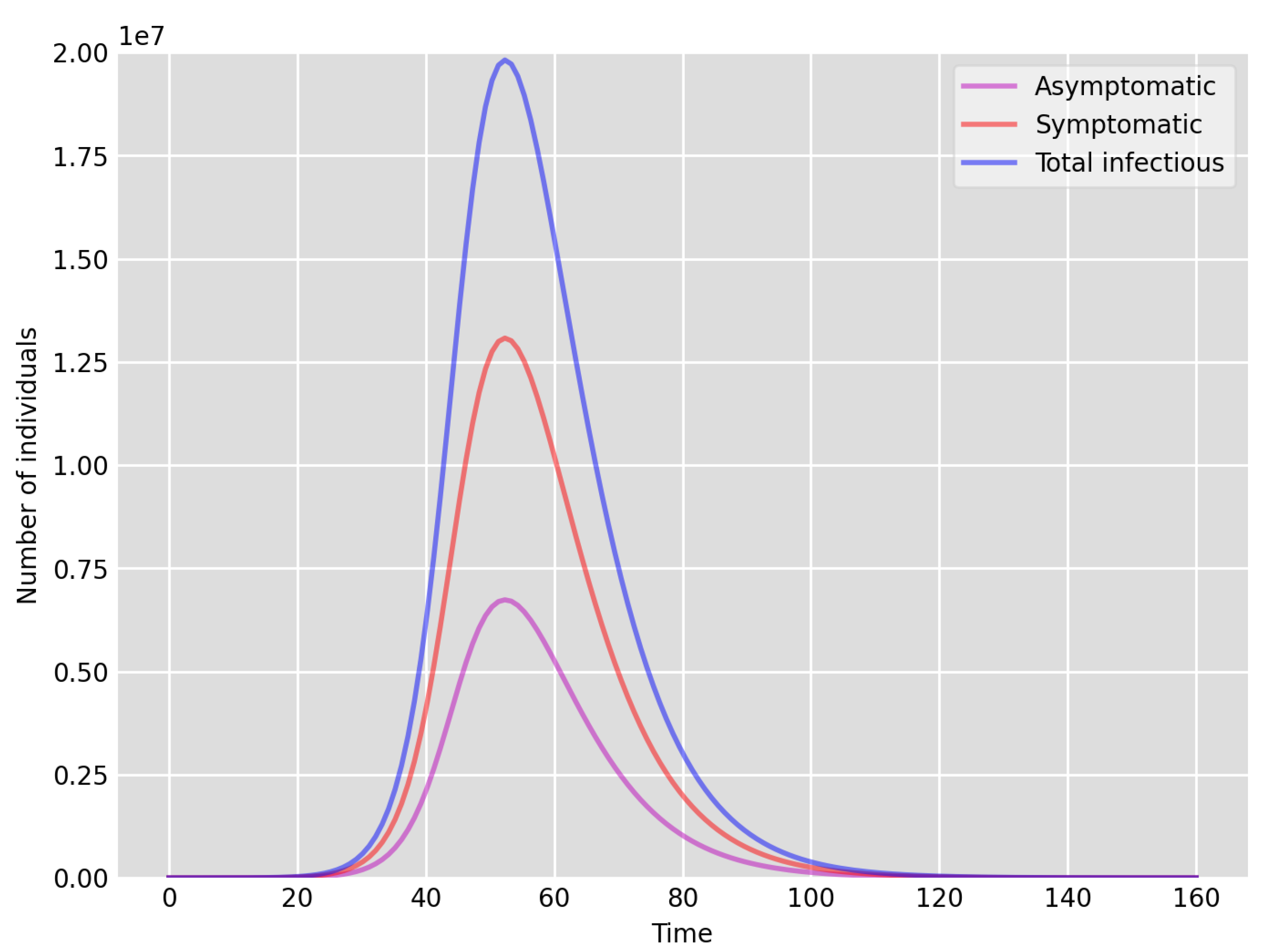
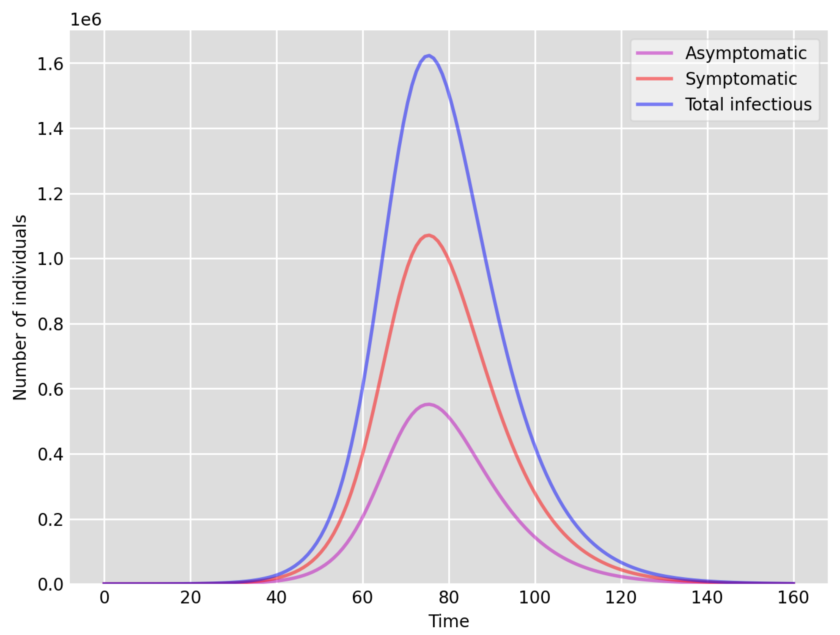
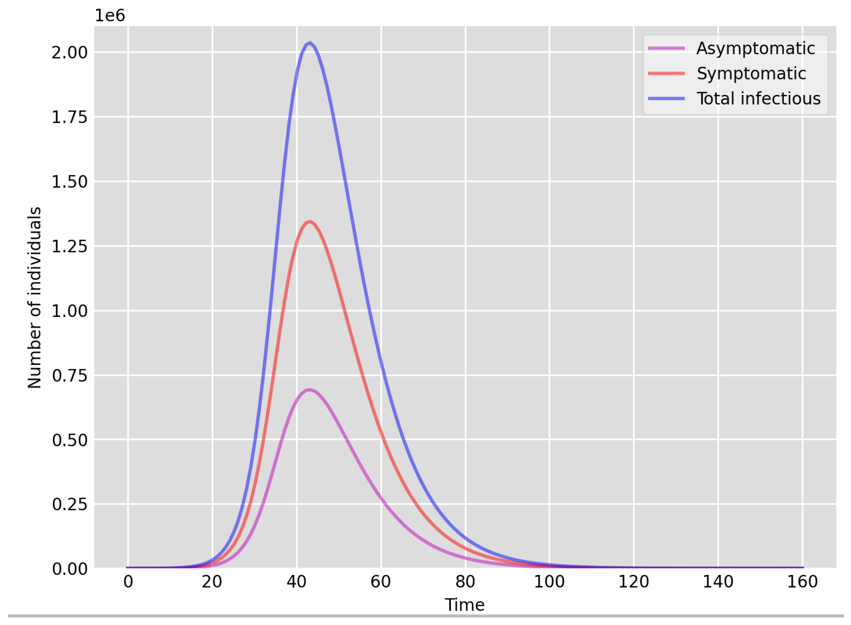
- Setup 1 () simulation results indicate very good agreement between the dates of the peak number of positive tests from the data and model simulation output for the total number of cases. In particular, test data indicate a peak at around 63 to 77 days (see Figure 2), while simulation outputs show infectious case numbers peaking at around 85 days (see Figure 1), and this is what one naturally expects as someone who tests positive may remain infectious for a further 5 to 10 days. While the wave takes place over a much shorter timescale in Setup 2, infectious individual numbers peak at around days 50–55 (see Figure 3), quarantining of a significant proportion of symptomatic individuals obviously slows down the spread of the disease. Hence, in principle, our simulation outputs would indicate that symptomatic infectious individuals adhered to self-quarantine rules during the first wave of the pandemic in the UK (indicated by the agreement with Setup 1).
- Comparing the peak number of cases in Setup 1 of (see Figure 1) to that against Setup 2, which is (see Figure 3), we can see that a reduction of approximately of peak numbers was achieved by moving from a very loose ) to a very strong () adherence to self-quarantine of symptomatic infectious individuals. Keeping in mind that we assumed that (a significant) two-thirds of exposed individuals become symptomatic, in our opinion, this is not a drastic change as one might hope for. Indeed, if for example only a third of exposed individuals become symptomatic, then our model (1) predicts that the impact of self-quarantine of symptomatic infectious individuals on peak case numbers would be negligible. However, self-quarantine has a much more significant impact during the early phase of the outbreak, which is due to the delay of the onset of the peak.
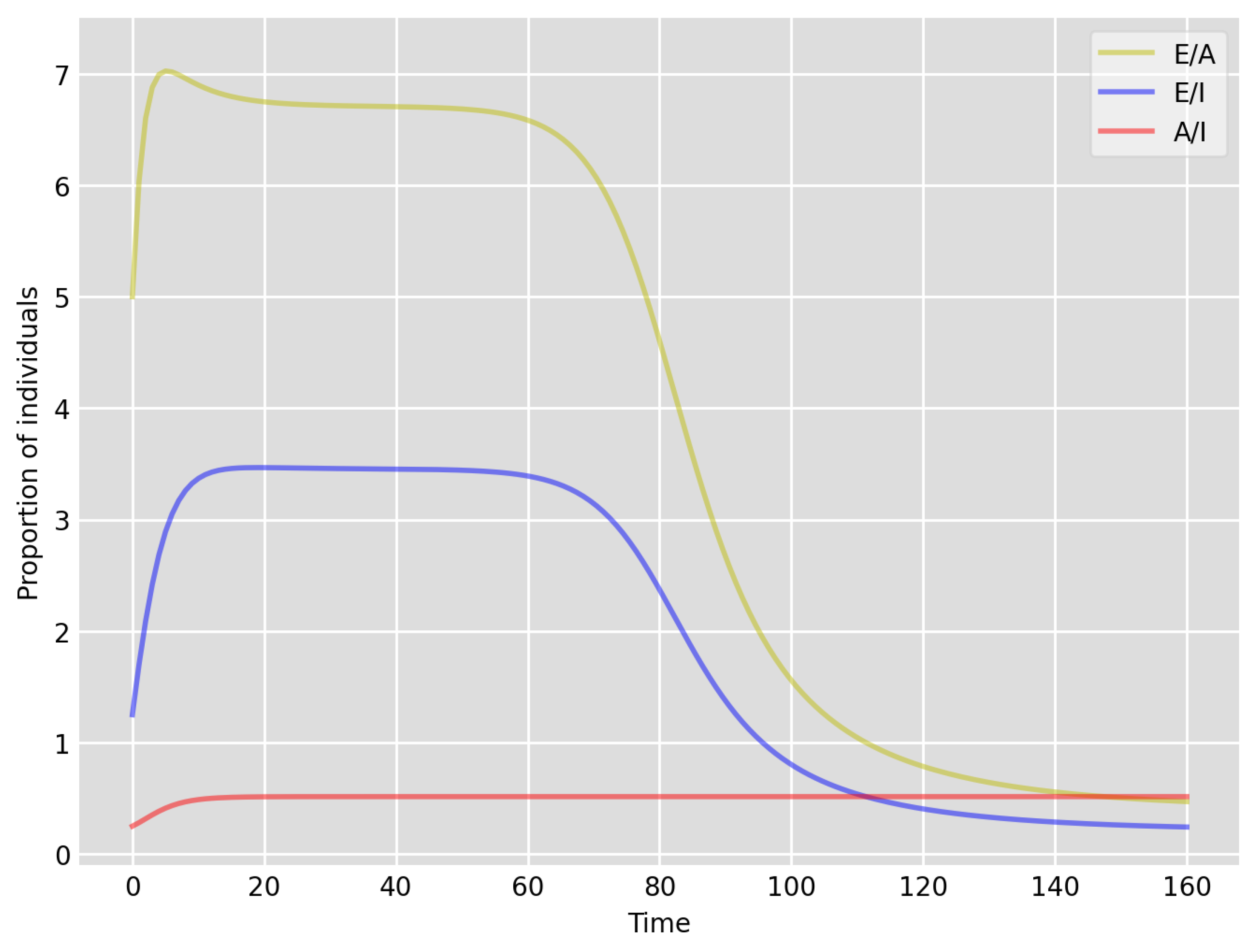
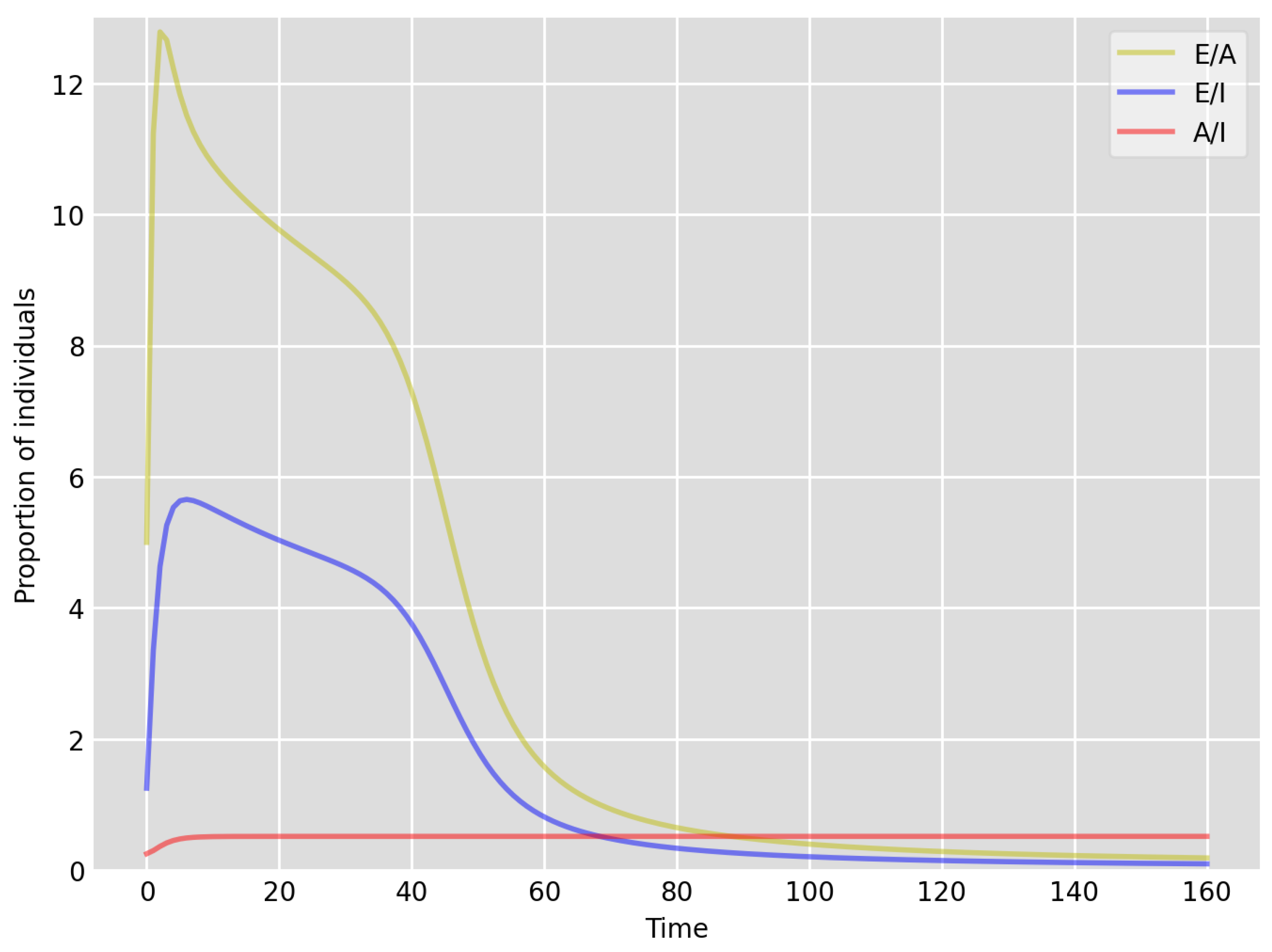
- Based on the literature, we choose the parameter value , meaning that, on average, two-thirds of the exposed individuals become symptomatically infectious. In both Setup 1 and 2, we observe that tends to the same constant as time goes to infinity, which is realistic, as this should be specific to the disease. Note that as one would expect, and simulations show that the ratio stabilizes very quickly.
- Comparing changes (Setup 1 to Setup 1 reduced vs. Setup 2 to Setup 2 reduced ), we can conclude that, in both cases, naturally, there is approximately a reduction in the total number of infectious cases (), due to the reduction in , the effective susceptible population, (compare Figure 1, Figure 2, Figure 3, Figure 4, Figure 5 and Figure 6). Infectious individual number peaks are also shifted (to an earlier date) by 13 days vs. 10 days in Setup 1 vs. Setup 2 (compare Figure 1, Figure 2, Figure 3, Figure 4, Figure 5 and Figure 6 and Figure 3, Figure 4, Figure 5, Figure 6 and Figure 7). Similarly, the reduction in the peak number of cases from Setup 1 reduced to that of Setup 2 reduced is approximately (compare Figure 6 and Figure 7), which is comparable to the reduction of from Setup 1 to Setup 2. Importantly, these simulation results may indicate that there is no significant combined effect of a national lockdown (modelled by the reduced effective susceptible population) and strong adherence to self-quarantine rules for symptomatic infectious individuals, when there is a significant proportion of asymptomatic infectious individuals (≈34%) and no mass testing, as was the case during the first wave of the pandemic in the UK. It is also clear from the simulations that all of the measures (e.g., national lockdown, (self)-quarantine) prolong the pandemic.
4. Discussion on —The Basic Reproductive Number
5. Outlook
Author Contributions
Funding
Institutional Review Board Statement
Informed Consent Statement
Data Availability Statement
Conflicts of Interest
References
- Danon, L.; Brooks-Pollock, E.; Bailey, M.; Keeling, M. A spatial model of COVID-19 transmission in England and Wales: Early spread and peak timing. medRxiv 2020. [Google Scholar] [CrossRef]
- Ghostine, R.; Gharamti, M.; Hassrouny, S.; Hoteit, I. An Extended SEIR Model with Vaccination for Forecasting the COVID-19 Pandemic in Saudi Arabia Using an Ensemble Kalman Filter. Mathematics 2021, 9, 636. [Google Scholar] [CrossRef]
- Liu, Z.; Magal, P.; Webb, G.F. Predicting the number of reported and unreported cases for the COVID-19 epidemics in China, South Korea, Italy, France, Germany and United Kingdom. J. Theor. Biol. 2021, 509, 110501. [Google Scholar] [CrossRef]
- Liu, Z.; Magal, P.; Seydi, O.; Webb, G.F. Predicting the cumulative number of cases for the COVID-19 epidemic in China from early data. Math. Biosci. Eng. 2020, 17, 3040–3051. [Google Scholar] [CrossRef]
- Liu, Z.; Magal, P.; Seydi, O.; Webb, G.F. A COVID-19 model with latency period. Infect. Dis. Model. 2020, 5, 323–337. [Google Scholar]
- Mwalili, S.; Kimathi, M.; Ojiambo, V.; Gathungu, D.; Rachel, M. SEIR model for COVID-19 dynamics incorporating the environment and social distancing. BMC Res. Not. 2020, 13, 352. [Google Scholar] [CrossRef]
- Kermack, W.O.; McKendrick, A.G. Contributions to the mathematical theory of epidemics, part I. Proc. Roy. Sot. Ser. A 1927, 115, 700–721. [Google Scholar]
- Kermack, W.O.; McKendrick, A.G. Contributions to the mathematical theory of epidemics, part II. Proc. Roy. Sot. Ser. A 1932, 138, 55–83. [Google Scholar]
- Diekmann, O.; Heesterbeek, J.A.P. Mathematical epidemiology of infectious diseases. Model building, analysis and interpretation. In Wiley Series in Mathematical and Computational Biology; John Wiley & Sons, Ltd.: Chichester, UK, 2000. [Google Scholar]
- Heesterbeek, J.A.P. The law of mass-action in epidemiology: A historical perspective. In Ecological Paradigms Lost: Routes of Theory Change; Cuddington, K., Beisner, B.E., Eds.; Elsevier: Amsterdam, The Netherlands, 2005. [Google Scholar]
- Simon, P.L.; Taylor, M.; Kiss, I.Z. Exact epidemic models on graphs using graph-automorphism driven lumping. J. Math. Biol. 2011, 62, 479–508. [Google Scholar] [CrossRef]
- Sharkey, K.J.; Kiss, I.Z.; Wilkinson, R.R.; Simon, P.L. Exact equations for SIR epidemics on tree graphs. Bull. Math. Biol. 2015, 77, 614–645. [Google Scholar] [CrossRef] [Green Version]
- Capasso, V.; Serio, G. A generalization of the Kermack–McKendrick deterministic epidemic model. Math. Biosci. 1978, 42, 43–61. [Google Scholar] [CrossRef]
- Calsina, À.; Farkas, J.Z. On a strain-structured epidemic model. Nonlinear Anal. Real World Appl. 2016, 31, 325–342. [Google Scholar] [CrossRef] [Green Version]
- Korobeinikov, A. Lyapunov functions and global stability for SIR and SIRS epidemiological models with non-linear transmission. Bull. Math. Biol. 2006, 68, 615–626. [Google Scholar] [CrossRef] [Green Version]
- Poirier, C.; Luo, W.; Majumder, M.S.; Liu, D.; Mandl, K.D.; Mooring, T.A.; Santillana, M. The role of environmental factors on transmission rates of the COVID-19 outbreak: An initial assessment in two spatial scales. Sci. Rep. 2020, 10, 17002. [Google Scholar] [CrossRef]
- Ferguson, N.M.; Laydon, D.; Nedjati-Gilani, G.; Imai, N.; Ainslie, K.; Baguelin, M.; Bhatia, S.; Boonyasiri, A.; Cucunubá, Z.; Cuomo-Dannenburg, G.; et al. Report 9: Impact of non-pharmaceutical interventions (NPIs) to reduce COVID-19 mortality and healthcare demand. Imp. Coll. Lond. 2020, 10, 491–497. [Google Scholar] [CrossRef]
- Qin, J.; You, C.; Lin, Q.; Hu, T.; Yu, S.; Zhou, X.-H. Estimation of incubation period distribution of COVID-19 using disease onset forward time: A novel cross-sectional and forward follow-up study. Sci. Adv. 2020, 6, eabc1202. [Google Scholar] [CrossRef]
- Bodas, M.; Peleg, K. Self-Isolation Compliance in the COVID-19 Era Influenced by Compensation: Findings from a Recent Survey in Israel. Health Aff. 2020, 39, 936–941. [Google Scholar] [CrossRef] [Green Version]
- Smith, L.E.; Potts, H.W.; Amlot, R.; Fear, N.T.; Michie, S.; Rubin, G.J. Adherence to the test, trace, and isolate system in the UK: Results from 37 nationally representative surveys. BMJ 2021, 372, n608. [Google Scholar] [CrossRef]
- Muchnik, L.; Pei, S.; Parra, L.; Reis, S.D.; Andrade, J.S., Jr.; Havlin, S.; Makse, H.A. Origins of power-law degree distribution in the heterogeneity of human activity in social networks. Sci. Rep. 2013, 3, 1783. [Google Scholar] [CrossRef] [Green Version]
- Rybski, D.; Buldyrev, S.V.; Havlin, S.; Liljeros, F.; Makse, H.A. Scaling laws of human interaction activity. Proc. Natl. Acad. Sci. USA 2009, 106, 12640–12645. [Google Scholar] [CrossRef] [PubMed] [Green Version]
- Prüss, J.W.; Wilke, M. Gewöhnliche Differentialgleichungen und Dynamische Systeme; Grundstudium Mathematik; Birkhäuser: Basel, Switzerland, 2010. [Google Scholar]
- Nagumo, M. Über die Lage der Integralkurven gewöhnlicher Differentialgleichungen. Proc. Phys. Math. Soc. Jpn. 1942, 24, 551–559. [Google Scholar]
- Office for National Statistics. Available online: www.ons.gov.uk/peoplepopulationandcommunity/populationandmigration/populationestimates (accessed on 1 September 2021).
- Bullard, J.; Dust, K.; Funk, D.; Strong, J.E.; Alexander, D.; Garnett, L.; Boodman, C.; Bello, A.; Hedley, A.; Schiffman, Z.; et al. Predicting Infectious Severe Acute Respiratory Syndrome Coronavirus 2 From Diagnostic Samples. Clin. Infect. Dis. 2020, 71, 2663–2666. [Google Scholar] [CrossRef] [PubMed]
- van Kampen, J.J.A.; van de Vijver, D.A.M.C.; Fraaij, P.L.A.; Haagmans, B.L.; Lamers, M.M.; Okba, N.; van den Akker, J.P.; Endeman, H.; Gommers, D.A.; Cornelissen, J.J.; et al. Duration and key determinants of infectious virus shedding in hospitalized patients with coronavirus disease-2019 (COVID-19). Nat. Commun. 2021, 12, 267. [Google Scholar] [CrossRef]
- Alene, M.; Yismaw, L.; Assemie, M.A.; Ketema, D.B.; Mengist, B.; Kassie, B.; Birhan, T.Y. Magnitude of asymptomatic COVID-19 cases throughout the course of infection: A systematic review and meta-analysis. PLoS ONE 2021, 16, e0249090. [Google Scholar] [CrossRef] [PubMed]
- Our World in Data. Available online: https://ourworldindata.org/ (accessed on 1 September 2021).
- Marschner, I.C. Estimating age-specific COVID-19 fatality risk and time to death by comparing population diagnosis and death patterns: Australian data. BMC Med. Res. Methodol. 2021, 21, 126. [Google Scholar] [CrossRef] [PubMed]
- Diekmann, O.; Heesterbeek, J.A.P.; Metz, J.A.J. On the definition and the computation of the basic reproduction ratio R0 in models for infectious diseases in heterogeneous populations. J. Math. Biol. 1990, 28, 365–382. [Google Scholar] [CrossRef] [PubMed] [Green Version]
- van den Driessche, P.; Watmough, J. Reproduction numbers and sub-threshold endemic equilibria for compartmental models of disease transmission. John A. Jacquez memorial volume. Math. Biosci. 2002, 180, 29–48. [Google Scholar] [CrossRef]
- Farkas, J.Z. Net reproduction functions for nonlinear structured population models. Math. Model. Nat. Phenom. 2018, 13, 32. [Google Scholar] [CrossRef] [Green Version]
- Calsina, À.; Farkas, J.Z. Positive steady states of evolution equations with finite dimensional nonlinearities. SIAM J. Math. Anal. 2014, 46, 1406–1426. [Google Scholar] [CrossRef] [Green Version]
- Thieme, H.R. Spectral bound and reproduction number for infinite-dimensional population structure and time heterogeneity. SIAM J. Appl. Math. 2009, 70, 188–211. [Google Scholar] [CrossRef]


| Model Parameters | p | ||||||
|---|---|---|---|---|---|---|---|
| Setup 1 | |||||||
| Setup 2 | |||||||
| Setup 1—reduced | |||||||
| Setup 2—reduced |
Publisher’s Note: MDPI stays neutral with regard to jurisdictional claims in published maps and institutional affiliations. |
© 2021 by the authors. Licensee MDPI, Basel, Switzerland. This article is an open access article distributed under the terms and conditions of the Creative Commons Attribution (CC BY) license (https://creativecommons.org/licenses/by/4.0/).
Share and Cite
Farkas, J.Z.; Chatzopoulos, R. Assessing the Impact of (Self)-Quarantine through a Basic Model of Infectious Disease Dynamics. Infect. Dis. Rep. 2021, 13, 978-992. https://doi.org/10.3390/idr13040090
Farkas JZ, Chatzopoulos R. Assessing the Impact of (Self)-Quarantine through a Basic Model of Infectious Disease Dynamics. Infectious Disease Reports. 2021; 13(4):978-992. https://doi.org/10.3390/idr13040090
Chicago/Turabian StyleFarkas, József Z., and Roxane Chatzopoulos. 2021. "Assessing the Impact of (Self)-Quarantine through a Basic Model of Infectious Disease Dynamics" Infectious Disease Reports 13, no. 4: 978-992. https://doi.org/10.3390/idr13040090