Creating a Robust SoC Estimation Algorithm Based on LSTM Units and Trained with Synthetic Data

Abstract

Creating SoC algorithms for Li-ion batteries based on neural networks requires a large amount of training data, since it is necessary to test the batteries under different conditions so that the algorithm learns the relationship between the different inputs and the output. Obtaining such data through laboratory tests is costly and time consuming; therefore, in this article, a neural network has been trained with data generated synthetically using electrochemical models. These models allow us to obtain relevant data related to different conditions at a minimum cost over a short period of time. By means of the different training rounds carried out using these data, it has been studied how the different hyperparameters affect the behaviour of the algorithm, creating a robust and accurate algorithm. To adapt this approach to new battery references or chemistries, transfer learning techniques can be employed.

1. Introduction

Systems capable of measuring the state of charge (SoC) have been around for practically as long as rechargeable batteries have [1]. The SoC shows the percentage of charge that is still available over the rated capacity of the battery [2]. SoC estimators are needed in all kinds of applications, since, for example, in the case of an electric vehicle, it will give the necessary information to know whether the car will reach the destination or whether it will need to be charged in an intermediate break [3].

To estimate the SoC of a battery, there are different methods, divided into three main groups. There are those referred to in the literature as (i) direct measurements, (ii) those defined as model-based, and finally (iii) computer intelligence algorithms [4,5].

Within the first group of direct measurements, the well-known Coulomb counting or Ah counting method can be found [6]. This method uses a current sensor that measures the current and then calculates the Ah discharged or charged and calculates the SoC of the battery with respect to the rated capacity. From the literature review, it is found that although this method is simple to implement, the accuracy of the estimation algorithm is directly influenced by the accuracy of the current sensor, its robustness to noise, and the initial SoC of the battery [7]. Moreover, if the current sensors are not accurate or have a certain reading error, this error will accumulate over time, which will cause the estimate to be further and further away from reality.

In addition to Coulomb counting, this first group also includes the open circuit voltage (OCV) estimation method [8]. This method estimates the SoC of the battery using the relationship between the OCV of the battery and its SoC. Although this method can be accurate, it is not feasible to use it in many applications, since for a correct estimation of the SoC it is necessary for the battery to be relaxed, which can mean a battery idle time of more than 3 h [9]. Furthermore, this method relies on an accurate voltage measurement, which can be challenging to obtain. Especially when the OCV curve of a battery has a low sensitivity to SoC evolution (for example, in lithium iron phosphate batteries), the accuracy of the voltage sensor can become deficient in evaluating the SoC change.

Model-based methods are often used to solve the problems of the aforementioned methods. These models use lithium-ion battery parameters for a model that mimics the behaviour of a battery cell. Primarily, the measured current, voltage, and temperature are fed to the ECM. A voltage is then estimated, and the error between the measured and estimated voltage is obtained. That error is then used to obtain the SoC value [10]. While these models provide satisfactory estimations in controlled conditions, such as specified battery type and constant ambient temperature, researchers are still searching for a unified model that describes the sophisticated behaviour of a battery in real operating conditions on site [11,12].

Finally, computer intelligence-based algorithms can be found. This group of algorithms has gained popularity in recent years due to two main factors. On the one hand, the speed of training has been reduced, due to increasingly faster GPUs, which has meant that training has been reduced from days or weeks to a few hours [13]. On the other hand, in recent years, due to improvements in connectivity and Industry 5.0, it has become easier to collect data during the application. Due to this ease of data collection, more training data are available, which enables the training of computer intelligence algorithms. In addition, the increasingly faster processing units in BMSs or the use of edge devices mean that SoC estimates can be made in a few milliseconds, if a trained model is used. In addition to all these factors, there are more and more resources, such as libraries or dedicated software tools, that help the implementation and use of these types of algorithms, thus simplifying development [14].

Computer intelligence-based algorithms include neural networks. Based on their nonlinear mapping and self-learning capabilities, some neural network techniques can execute the lithium-ion battery SoC prediction task [15]. However, due to their relatively basic structure, the feed-forward neural networks are marked by slow convergence and a poor capacity to handle time series data. In contrast, deep learning techniques can handle time series data, but they also have the drawback of creating too complex and therefore difficult-to-apply algorithms [16,17].

The algorithms called recurrent neural networks (RNN) show high robustness to dynamic loads, nonlinear dynamic nature, hysteresis, aging, and parametric uncertainties [18]. While making use of historical information, the RNN presents a better estimation of the battery SoC when compared to other neural networks [19]. 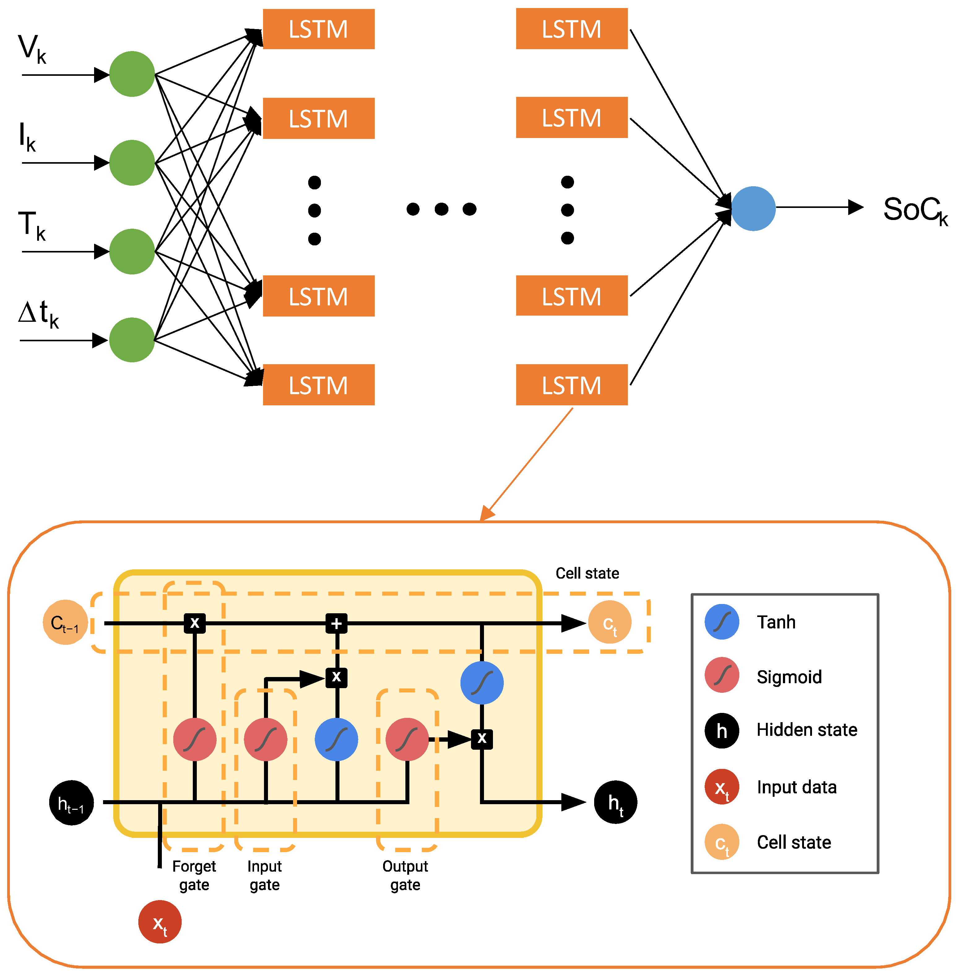But RNNs are unable to describe long-term dependencies because they suffer from a vanishing gradient effect, which causes neural networks to have a short-term rather than a long-term memory [14]. To overcome this problem, another type of unit called long short-term memory (LSTM) is used by using a memory cell. An LSTM decides what to remember and what to forget, using different gates (input, output, and forget) [20].

Although training times have been reduced due to powerful GPUs, the development of SoC estimation algorithms requires several tests to be performed on batteries under different operating conditions (temperature, currents, SoH or SoC), usually in a laboratory environment, which is both costly and time consuming. A major problem in this field of research is that an estimation model developed for a particular reference cell is not necessarily suitable for a different cell (different manufacturer, size, chemistry, etc.). This limitation implies that every time, an estimation algorithm must be developed for new cells, and all the laboratory tests must be started anew, which implies a significant investment in resources.

Since obtaining this volume of data can be costly and requires a lot of laboratory testing, techniques such as transfer learning (TL) can be used [21,22,23]. The use of neural networks in conjunction with the TL technique allows the use of data and prior knowledge generated from references of previously tested or deployed cells, whether or not they are cells or batteries of different chemistry, capacity, or format. In order to achieve a successful TL, it is necessary to create a base model that is robust and has been trained with as many conditions as possible, so that the amount of data or conditions required to perform the TL on a new Li-ion battery chemistry or reference will be reduced [24,25]. Therefore, the aim of this paper is to create a robust base model that can then be adapted to any battery using the transfer learning technique and a limited amount of training data.

As mentioned above, to achieve a robust and accurate SoC estimation algorithm, it is critical to have an extensive database in which the battery has been cycled under a wide range of temperature and current conditions. Getting this data through laboratory testing can be time consuming and expensive. To obtain such a database as quickly and cost-effectively as possible, a well-accepted electrochemical model was employed. This model is based on simulating the behaviour of an LCO/graphite-based cell known as the Doyle cell [26]. By means of such an electrochemical model, the voltage response to a wide range of operating conditions can be simulated, instead of measuring experimentally within lab tests the actual performance of such a cell. This approach allows significantly shortening the amount of time required to generate the dataset required to train the SoC estimation algorithm.

Thus, this article is organized as follows: (i) the architecture based on computer intelligence to create the SoC estimation algorithm will be explained; (ii) it will be explained more specifically which data are used to train the algorithm, how they have been obtained, and how the partitioning of these data for training, validation, and testing has been performed; (iii) thirdly, the results obtained from different configurations of the neural network and the results obtained from the selected neural network will be explained; (iv) finally, the conclusions drawn from this study will be presented, and the results obtained from the selected neural network will be presented.

2. SoC Estimation Algorithm

In this section, an LSTM network is proposed as a way to model the nonlinear dynamics of lithium-ion batteries and compute the SoC of the battery using observed variables such as temperature, current, and voltage. Time series data processing is better suited for the LSTM units since they use hidden cell memories to store data from previous inputs. The LSTM network is discussed in depth below.

2.1. LSTM Network

The proposed SoC estimator architecture is shown in Figure 1. It consists of an input layer, an LSTM layer, a fully connected layer, and an output layer. There are four variables that are used as input for the network to perform the SoC estimation: the voltage (V_k), the current (I_k), the ambient temperature (T_k), and the time step (Δt_k). It has been considered very useful to include this last input, since the time step may vary depending on the application and its hardware. For example, an application with fast dynamics, where the current changes rapidly, will need a faster sampling time in order to correctly estimate the SoC, whereas in an application where the dynamics are slow, such a fast sampling time will not be necessary.

Data flow from the input layer to the LSTM where the most influential temporal relationships between the input variables will be found. Then, data flow into a fully connected layer where the output value is calculated, giving the estimated SoC value in the output layer.

2.2. Long Short-Term Memory Units

LSTMs are employed to resolve the gradient vanishing issue of the RNN, as it has been described in Section 1. To reduce the gradient vanishing rate and capture long-term dependencies, the LSTM creates a new activation function. The LSTM’s core principle is the cell memory, which, if unpacked, streams down the entire chain subject to an affine transformation. The architecture of a typical LSTM unit is illustrated in Figure 1, where c_t denotes the unit memory at time t.

As depicted in Figure 1, LSTM networks use three different gates. The input gate decides what information will be passed to the cell state c_t. The forget gate controls which information should be saved and which should be forgotten from the previous cell state. The output gate, on the other hand, decides what the next hidden state should be [28,29].

The following steps are taken during an LSTM unit’s forward pass: first, the previous hidden state and the new input data are concatenated or combined (called from now on “combination”). That combination flows to the forgetting layer, where non-relevant data are removed. Next, a candidate layer is created using the combination. The combination in turn enters the input layer where it is decided which candidate data should be added to the new cell state. Thus, after computing the forgetting, candidate, and input layers, the new cell state is computed with those vectors and the previous cell state. Then, the output is computed. Finally, the new hidden state is computed by pointwise multiplying the output and the new cell state [30].

The entire system, including LSTM layers, has been implemented using the Python programming language and TensorFlow, a robust open-source deep learning framework. A key element of the system is hyperparameter tuning, a process that refines model parameters to enhance performance, as will be depicted more deeply in Section 4. This procedure has been done using the Weights & Biases (W&B) library, a tool renowned for its capabilities in tracking and visualizing metrics. This combined approach ensures a system with optimized LSTM layers for superior accuracy and efficiency.

3. Dataset

Cell behaviour and mechanisms occurring inside batteries can be analysed through electrochemical models to hasten the data-driven model’s development. As mentioned in Section 1 of this article, the dataset used to train, validate, and test the neural network has been obtained by using a physics-based model. The pseudo-two-dimensional model (P2D) has been implemented considering the cell described by Doyle et al. in [24] as a compromise between accuracy and fast computational time to allow the required inputs for the data-driven model. The model can simulate any insertion cell, if physical properties and system parameters are given, and is based on the porous electrode and concentrated solution theory. It is not possible to describe perfectly the complex multiphysics behavior of batteries, and for this reason, a clarification of the continuum model approach and model assumptions must be well defined to establish the model framework. More detailed information on the P2D model description can be found in [24]. This continuum model consists of a 1D macroscopic model coupled with a pseudo dimension.

As depicted in

Table 1. Simulated profiles for training/validating/testing the SoC estimation algorithm.

Profile Type	Used for	Temperatures	C-Rate CHA	C-Rate DCH
Designed profile	Training	0 °C, 10 °C, 25 °C and 45 °C	0.05C, 0.2C, 0.5C and 1C	0.05C, 0.2C, 0.5C, 1C, 2C and 4C
HPPC	Validation	0 °C, 10 °C, 25 °C and 45 °C	Pulses of 1C and 2C	Pulses of 1C and 2C
Driving cycles	Test	0 °C, 10 °C, 25 °C and 45 °C	Driving profiles (NEDC, WLTC, US06, HWFET, NYCC, and UDDS)

, three different types of profiles were simulated, with the purpose of subjecting the SoC estimation algorithm to operating conditions of a diverse dynamic nature.

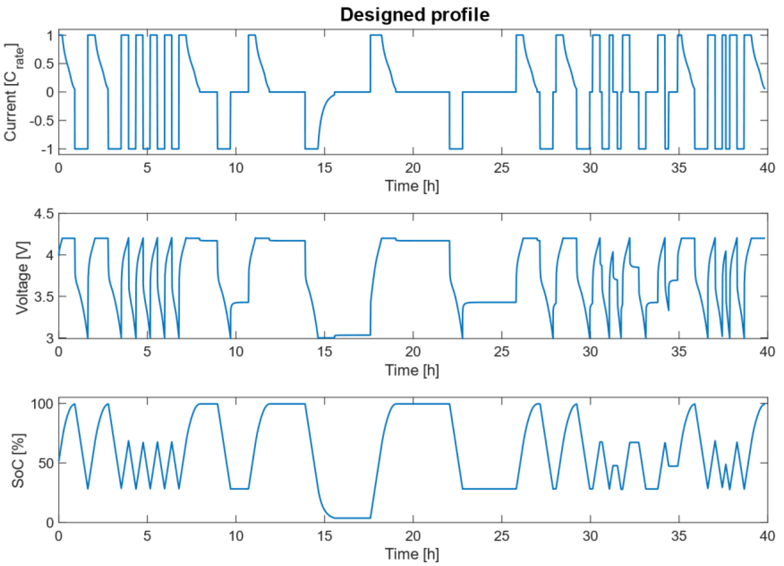
The first profile was specifically designed to train the neural network. Throughout the profile, the cell was taken to different SoC states performing constant current (CC) and constant current–constant voltage (CC–CV) charges and discharges. Finally, pause times were included so that the algorithm could learn how all these events affect the battery SoC estimation. This profile was simulated at different temperatures and different charge and discharge currents. More specifically, it was simulated at four different temperatures (0 °C, 10 °C, 25 °C, and 45 °C), at four different charge C-rates (0.05C, 0.2C, 0.5C, and 1C) and six different discharge C-rates (0.05C, 0.2C, 0.5C, 1C, 2C, and 4C). In total, the cell was simulated under 24 different conditions. Figure 2 shows an example of the simulation corresponding to 25 °C, 1C charge, and 1C discharge.

The second simulated profile corresponds to a hybrid pulse power characterization (HPPC) test profile. Although this type of test is not necessary when training the neural networks, it was implemented because it can be very interesting to see in the phase of validation if the algorithm has been able to learn the effect of the battery’s internal resistance when introducing current peaks in both charging and discharging phases.

The test consists of applying charge and discharge current pulses of 17 s sequentially at 1C and 2C over the whole voltage range of the cell, starting from fully charged to completely discharged at 5% SoC steps. Then, the same process is applied but starting from a discharged battery until fully charged. The test was repeated under four different ambient temperature conditions (0 °C, 10 °C, 25 °C, and 45 °C).

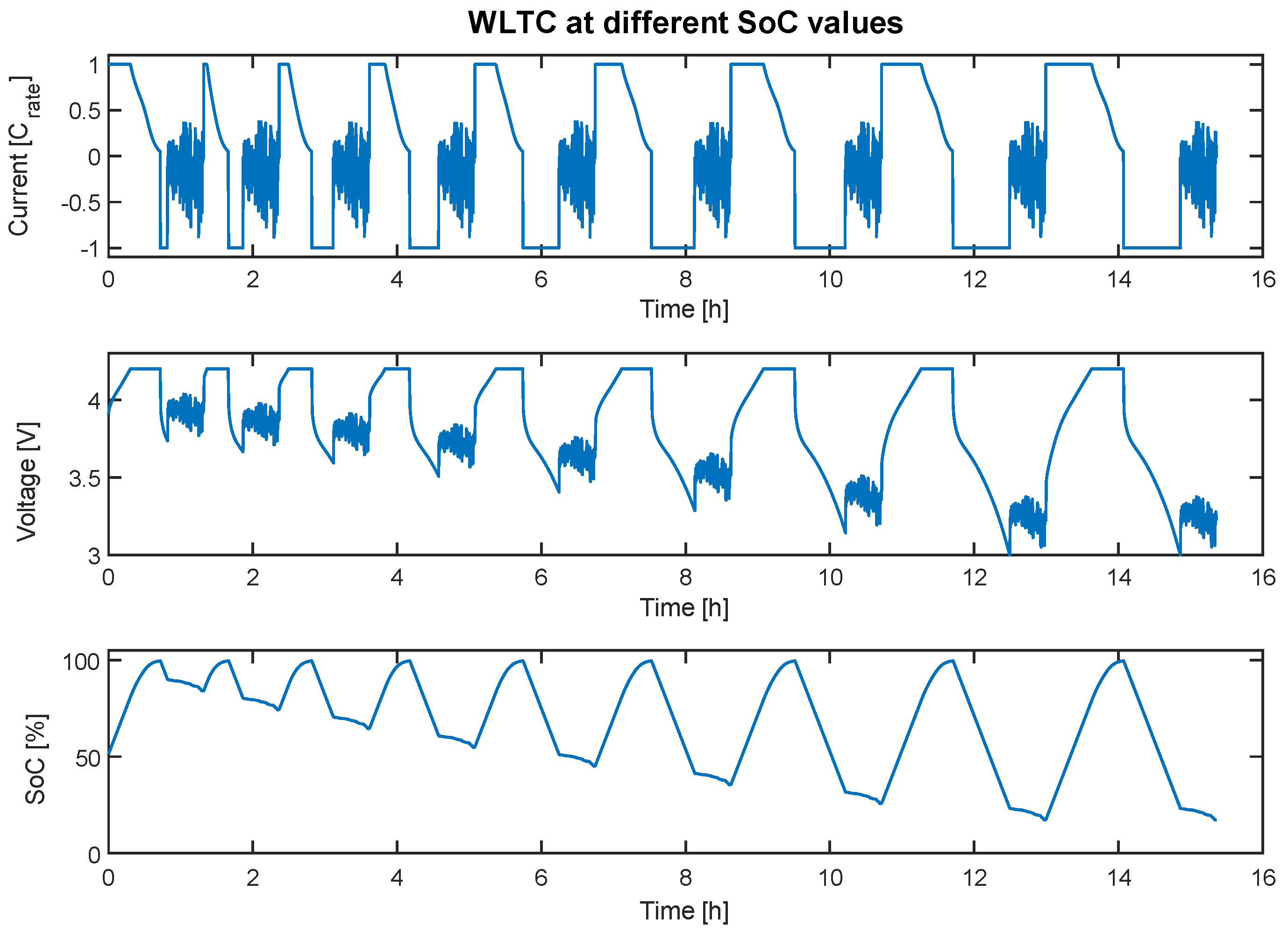
Finally, the battery was simulated under standardised driving cycles. The battery was charged up to 100% SoC, and then standard driving profiles were simulated. Once the profile was completed, the battery was charged at a constant current up to 100% SoC and discharged at a constant current 5% SoC, and the same profile was simulated again. The same process was repeated, discharging after each charge 5% more SoC than the previous time until the lower voltage limit of the battery was reached. This same test was repeated for each of the six simulated driving cycles (NEDC, WLTC, US06, HWFET, NYCC, and UDDS) and at four different temperatures (0 °C, 10 °C, 25 °C, and 45 °C). In Figure 3, the cycle is depicted that corresponds to the WLTC driving cycle at 25 °C, starting at a different SoC each time.

One of the most important points when training a neural network is the correct portioning of training, validation, and test data [31,32]. In the present study, a test has been specifically designed and used to train the neural network (the first one presented in Figure 2). The HPPC test has been used to validate the neural network, since this type of test includes, in addition to the charge and discharge pulses, constant charge and discharge phases, making it a good test to observe the behaviour of the neural network during training. Finally, the driving cycle tests are the ones that most closely resemble a real-life application; they are the ones that have been used to test the neural network.

4. Algorithm Configuration and Hyperparameter Tuning

To create the most accurate and robust SoC estimator possible, different parameters that compose the algorithm must be carefully selected. To do so, it is necessary to perform different trials by changing the different parameters in order to get the configuration that best suits the problem. For this purpose, in this study, different tests were performed by changing—as described below—some parameters, such as the windowing of the data, different dropout values, or the number of neurons composing the LSTM layer. Thus, the results obtained from the different trainings and the steps followed to find the configuration that best suits the application are presented below.

The MAE will be employed to determine the optimal value of the different hyperparameters in the different tests that are going to be performed. The MAE is calculated according to the following formula:

$$MAE=\frac{1}{N}\sum _{i=1}^N\left|y_i-\widehat{y_i}\right|$$

(1)

where N is the number of examples, y_i is the real SoC value, and y_i is the estimated SoC value.

4.1. Window Length

Data windowing, also known as sequence chunking or sliding window, is a crucial preprocessing technique used in long short-term memory (LSTM) networks and other sequence-based models. It involves dividing the input time series data into smaller windows, which are then fed into the LSTM network. This approach enables the model to capture temporal dependencies and patterns within the data, allowing it to make more accurate predictions for time series forecasting tasks [33].

The choice of window size is an important factor that can significantly impact the performance of an LSTM network. A smaller window size may not capture long-term dependencies in the data, leading to inaccurate predictions. On the other hand, a larger window size may increase the complexity of the model, resulting in longer training times and a higher risk of overfitting.

4.2. Dropout

Dropout is a regularisation method in which the input and recurrent connections are probabilistically excluded from activation and weight updates during training of a network. This procedure typically has the effect of reducing overfitting and improving the performance of the model [34].

4.3. Batch Size

Batch size is an important parameter to consider, as it can significantly impact the model’s performance and training time. The batch size refers to the number of training samples that are processed simultaneously during each iteration of the training process. By adjusting the batch size, one can control the trade-off between computational efficiency and the granularity of weight updates [35].

A smaller batch size can lead to more frequent weight updates, which may result in faster convergence and improved generalization performance. This possibility exists because smaller batches introduce more noise into the gradient estimates, which can help the model escape local minima and explore the solution space more effectively. However, smaller batch sizes also require more iterations to process the entire dataset, which can increase the overall training time. On the other hand, larger batch sizes can lead to more stable gradient estimates and faster training times due to the increased computational efficiency of processing multiple samples at once [36].

4.4. LSTM Layer Size and Number of Hidden Layers

It is very important to find an adequate relationship between the number of layers of the neural network and the number of nodes in each layer. On the one hand, a neural network with only one layer but with many nodes will tend to memorize the output but will not be good at generalizing, so when trying to estimate situations not contemplated during the training, it will have a poor performance. On the other hand, increasing the number of layers will make the network have a better generalization capacity, since through the different layers it will learn the necessary features to estimate correctly from the inputs. However, if the number of layers is too high, or in other words, if the network is too deep, there is a risk because the network will tend to overfit, so that it will be very accurate on training data but very inaccurate on test data [37,38].

Therefore, it is necessary to find an optimal relationship between the number of nodes in each layer and the number of layers. Moreover, the larger the network, either because it has more nodes or because it is deeper, the longer the time required for the network to be trained.

4.5. Hyperparameter Tuning

In order to perform hyperparameter tuning and achieve the best possible hyperparameters, Bayesian optimisation has been used to effectively find the best hyperparameters for the network. Bayesian optimisation is a technique for hyperparameter tuning that leverages Bayesian logic to reduce the time required to obtain an optimal parameter set, improving the performance of test set generalization tasks. This optimization technique takes into account previously seen hyperparameter combinations when determining the next set of hyperparameters to evaluate. This approach allows the algorithm to intelligently explore the hyperparameter space, focusing on regions that are more likely to yield better results and avoiding areas that have already been proven suboptimal [39,40].

The core of Bayesian optimization lies in the use of Gaussian processes to model the objective function, which represents the relationship between hyperparameters and model performance. By maintaining a probabilistic model of the objective function, Bayesian optimization can estimate both the mean and the uncertainty of the performance for any given hyperparameter combination. The algorithm then selects the next hyperparameter set to evaluate based on an acquisition function. This approach enables Bayesian optimization to efficiently search the hyperparameter space, often leading to quicker convergence and better generalization performance on test sets compared to traditional tuning methods [36].

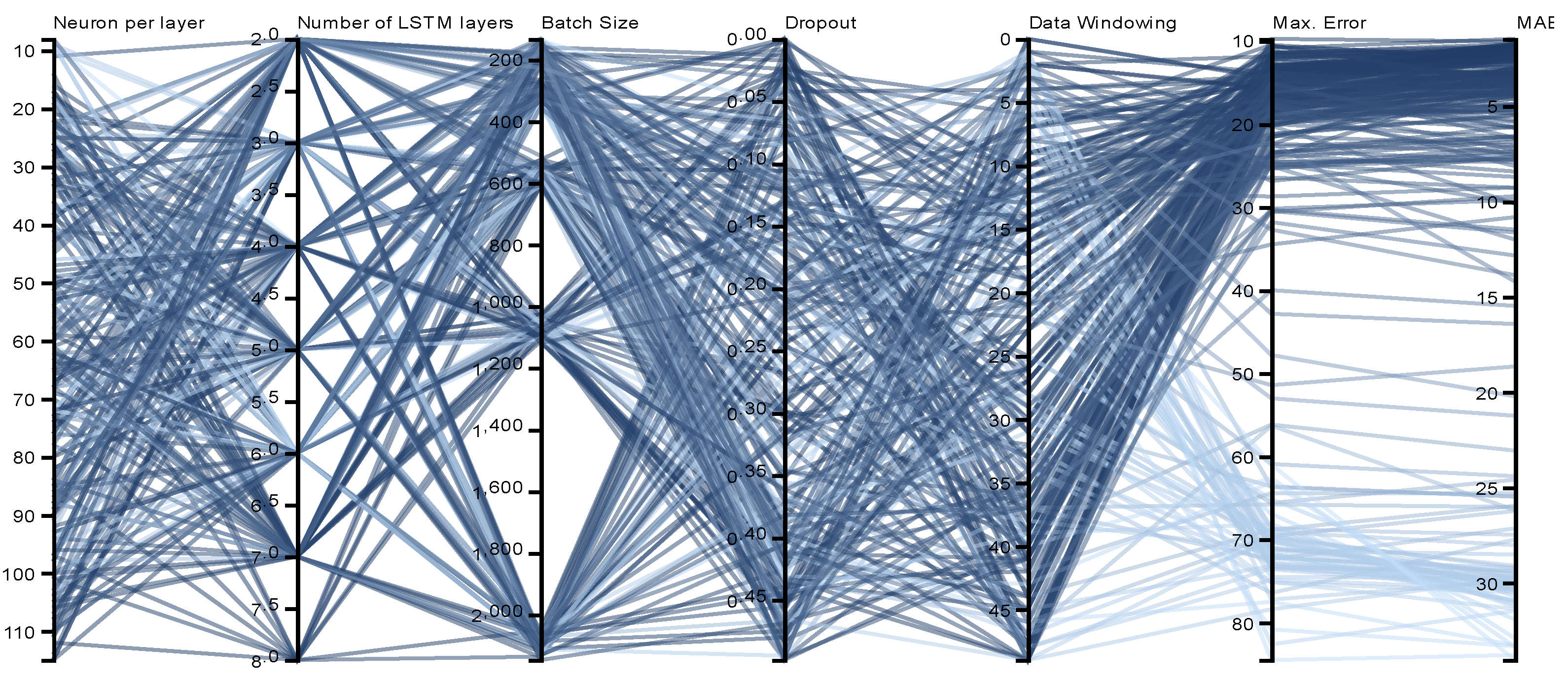
Figure 4 shows the results obtained after performing the Bayesian optimisation. During the optimisation, the different hyperparameters listed throughout this Section 4 have been tested. For example, as depicted in Figure 4, various network sizes were tested, ranging from a single LSTM layer to eight LSTM layers and from eight neurons per layer to 120 neurons per layer. The results indicate that the optimal configuration, which yielded the best outcomes, consists of three LSTM layers with 50 neurons per layer.

From all the different tests performed, the one that showed the best compromise between the MAE and the maximum error was chosen.

Table 2. Network hyperparameters.

Window length	15
Dropout	0
Batch Size	512
LSTM Layers	3
LSTM units per layer	50

shows, therefore, the configuration of hyperparameters that will form the network.

5. Results

After performing all the tests, the parameters that yielded the best results were selected, and 10 extra training sessions were carried out in order to select the one that produced the best result.

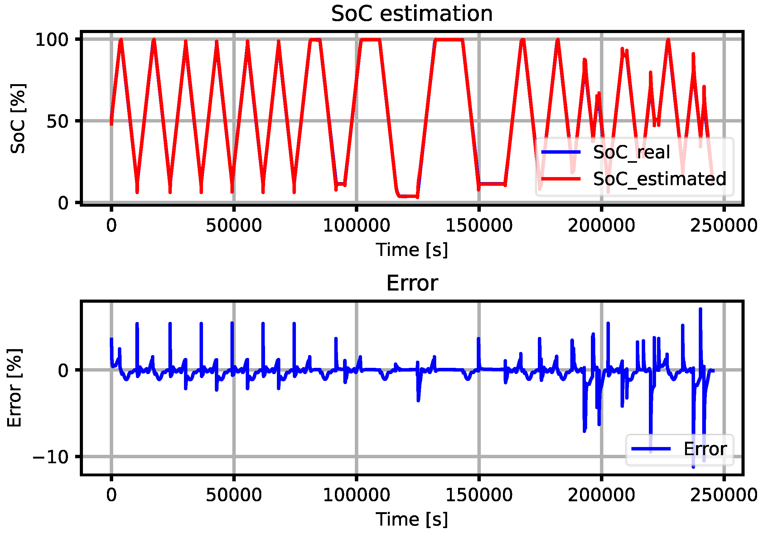
Figure 5 shows an example of how the algorithm behaves with the training data. In this case, it shows the results for the profile designed at 25 °C and charge and discharge at 0.5C. The MAE error in the training data is 1.48% and in the validation data 1.54%; the maximum error is 10.85% for training and 13.21% for validation.

The figure provides an illustration of how effectively the algorithm tracks the actual SoC with an MAE of less than 1.5%, demonstrating a high level of accuracy. However, it is noteworthy that there are instances of elevated error peaks, particularly when alterations in the current occur. This anomaly becomes even more pronounced during periods of rapid battery dynamics, as evidenced in the concluding stages of the specified cycle.

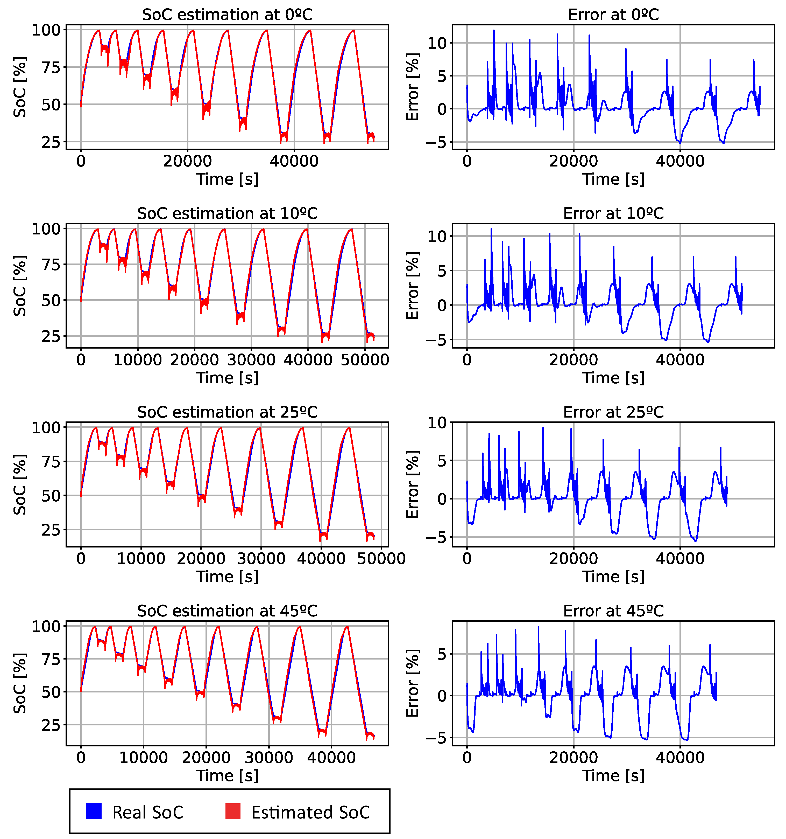
As mentioned in Section 4, the data corresponding to the EV profiles have been used to test the algorithm. Figure 6 shows how the algorithm behaves and the error it yields for the WLTP profile at 0 °C, 10 °C, 25 °C, and 45 °C.

The left column of Figure 6 showcases the estimations made by the algorithm (represented in red) juxtaposed against the actual data (depicted in blue). From this comparison, it becomes apparent how closely the algorithm mirrors the true trajectory of the SoC. A notable discrepancy between the estimated SoC and the real SoC is observed during the transition from the CC discharge phase to the WLTP cycle. Despite this occurence, the disparity is largely momentary and is swiftly rectified by the algorithm autonomously.

The algorithm’s performance was found to be significantly more robust at elevated temperatures, specifically at 45 °C, where it achieved the smallest error. This finding suggests a temperature-dependent behaviour of the algorithm, indicating it potentially has greater accuracy in high-temperature environments.

As can be seen in Figure 6 and in

Table 3. Model estimation MAE and maximum error for the different datasets.

	MAE	Max Error
Training	1.48%	10.85%
Validation	1.54%	13.21%
Test	1.64%	11.50%

where the results obtained by the algorithm created are presented, it can be seen that the MAE always remains below 2% and that the maximum error remains close to 11%. From the results obtained in the training, validation, and test data, it can be concluded that the network has not suffered from overfitting, as the results obtained are similar in all cases.

6. Conclusions and Future Work

In this paper, an SoC estimator based on neural networks has been created; more specifically, LSTM nodes have been used. As it has been observed throughout this article, the use of this type of neuron makes the network behave especially suitably when used for time series data. One of the main benefits of using neural networks with respect to other methods used in the literature is that it is not necessary to use or perform any specific test to ensure the correct operation of the algorithm, since this type of estimator automatically searches for the relationship between the input data and the output.

One of the big drawbacks of neural network-based algorithms is that they need a large amount of data to correctly find the relationship between input and output data. To feed the neural network, this study uses data from an electrochemical model. The benefit of using this type of model to generate the data necessary for a correct training of the network is that it allows the creation of a large database in which various conditions (current, temperature, etc.) are taken into account, using a fraction of the cost of money and time that they would if carried out in a laboratory.

Throughout this article, the importance of a correct adjustment of the hyperparameters (number of layers, nodes, etc.) has been noted. Equally important is the correct use of the data and a division between training, validation, and test data. For the training of the algorithm, in this article, a specific profile has been created to train the neural network (presented in Section 3). This profile takes the cell to different SoC and voltage conditions, as well as different pause times, so that the network is able to learn how a cell behaves under different operating conditions. Within the training, but as validation data, data from HPPC tests have been used, as this type of test includes DC and peak current charges and discharges. Finally, for the algorithm test, realistic car profiles have been used, as this type of test resembles the operation of a cell under real operating conditions.

From the results obtained, it can be concluded that the algorithm has a great capacity to extract the relationships between the different inputs to correctly estimate the SoC, since the profiles used for testing are more dynamic than those used in training, which means a higher level of complexity for the network. Despite this, the algorithm estimates the SoC with an MAE of less than 1.7% and maximum peak errors of 11.5% for the testing data.

The algorithm, despite its merits, does have certain limitations and considerations that warrant attention. Since it has been trained using synthetic data devoid of noise, it becomes imperative to assess its performance when exposed to noisy signals. Additionally, the computational power required for the algorithm to run effectively on onboard hardware is another crucial factor to consider. Upon analysing the results, it is evident that certain points, particularly during the transition from discharge to charge, exhibit a higher error between the estimated and actual SoC, reaching up to 10%. This discrepancy could potentially be mitigated by implementing filtering techniques to enhance the accuracy of the estimated SoC values. By addressing these concerns, the algorithm’s performance can be refined and more precise SoC estimations ensured.

Moreover, it is essential to investigate how the algorithm performs when applied to other battery chemistries, such as LFP (lithium iron phosphate). By addressing these aspects, comprehensive understanding of the algorithm’s capabilities and potential areas for improvement can be gained.

Finally, considering the great number of different conditions that have been used to develop this model, it is believed that this model can be a great base to implement the transfer learning technique and thus be capable of applying all the knowledge acquired during training to create SoC estimators for other batteries by retraining with a reduced amount of data.

To propel the algorithm’s advancement, the logical next steps would involve gathering data from actual cells in real-world applications or controlled laboratory settings. By leveraging the algorithm outlined in this article, one could retrain its layers to accommodate fresh data obtained from real cells. This iterative process of data collection and algorithm refinement is crucial for enhancing the algorithm’s performance and adaptability in practical scenarios.