Mixed Linear Model of a Safety Dispatch Model in an Active Distribution Network for Source–Grid–Load Interactions

Abstract

There are a large number of plug-and-play loads in an active distribution network, such as EVs(Electric Vehicles), energy storage, solar power, etc. Due to the lack of security control methods for each terminal node and the lack of distributed power voltage control methods, the large number of loads brings a huge challenge to the security of the distribution network. At present, some regional distribution networks dominated by new energy in China have long-standing problems, such as high voltage impact and frequency flickering, which are extremely harmful to electric equipment, and the resulting load-side accidents have brought huge economic losses. Therefore, research on an optimization model of the source–grid–load interaction in the active distribution network considering the safety characteristics, especially the voltage of the system, will help to improve the quality of the grid dispatch. In this paper, the safety limits of the independent operation of a source network loaded on three sides are used as the operating constraints of the system, and the social welfare of the interaction is maximized as the goal. A joint optimization modeling after the independent solution of the three sides is used as the core means, a heuristic algorithm is used to solve the overall optimization of the whole system, a scheduling optimization model that meets the system security goals is constructed, and this model is used to guide the operation strategy of each node in the system. The Lagrangian relaxation factor is introduced for structural optimization, and finally, the simplified 36-node model of the actual power grid is used for verification. The results show that under the goal of ensuring the economy of the system, the system voltage is controlled within the specified range of the safe operation of the system, which can meet the safety needs of the interaction.

1. Introduction

Power distribution systems around the world are experiencing a large-scale deployment of distributed energy (DER), such as renewable and nonrenewable distributed power generation (DG), distributed energy storage systems (DESS), plug-in electric vehicles (PEV), and micro-combined heat and power (CHP) plants [1]. In recent years, due to the encouragement and stimulus of governments around the world, the penetration rate of renewable energy has continued to rise. This rapid onset of DERs has brought about a paradigm shift in the way that conventionally passive distribution networks have been planned and operated [2], leading to the advent of active distribution networks (ADNs). ADNs are essentially driven by advanced information and communication technologies (ICT) and active network management (ANM), which facilitate the DG control and optimization [3], the distributed storage utilization [4], multi-energy integration [5,6], the coordinated control of various system elements, and the demand response programs [7,8].

The conventional DNP is incapable of providing an adequate planning solution for active distribution networks. This is because the DG interconnections transform the distribution network operation in terms of bidirectional power flows, voltage rises and fluctuations, aggravated fault levels, lower power losses, and reliability and stability problems [9]. Moreover, the intermittent generation of the nondispatchable renewable DGs imposes operational uncertainties on the power availability. Numerous other factors including load variability, demand growth, and electricity market prices introduce further operational uncertainties to distribution system planning. Note that operational uncertainty is the level of accuracy with which an input parameter of the planning problem can be forecasted [10]. The compounded effect of these uncertainties can bring about several operational and control challenges: for instance, protection degradation and stability issues [11]. The typical thorough treatment of uncertain input parameters of the planning problem can either lead to computational inefficiency or intractability; hence, this problem demands the application of accurate and efficient uncertainty modelling techniques [12]. Security deals with network responses to all kinds of disturbances, and so is concerned with network dynamics and transient operating conditions, such as voltage instability in the event of major generation and transmission outages [13]. The persistent expansion of smart grids makes the reliability assessment more complex and challenging. Increasing distributed energy resources improves the power supply adequacy due to their inexhaustible nature, but it can reduce the security as a result of power injection and the power flow increase in the lines in the distribution network [14]. To achieve acceptable and optimal reliability, the old-fashioned ‘fit and forget’ strategy can no longer be applied in modern smart networks. The DERs’ output powers must be frequently changed in different time horizons and operating conditions, where the network must be continuously reconfigured, i.e., network reconfiguration, to address such changes when needed [15]. This poses a huge challenge to distribution network security [16].

Currently, source–grid–load interaction has become a better method for active distribution network dispatch [17], but due to the large difference between the power dispatching method and the main grid, the unit generally suffers from a lack of adjustability. Under normal circumstances, there will be many safety issues, such as machine terminal voltage rise, system frequency fluctuations, voltage flickering, and other related power quality issues [18]. Among them, the problem of voltage lifting is particularly serious. In order to maximum the output of the generator, the unit will raise the voltage, leading to the high voltage of the whole grid, and at the same time raising the safety risk [19,20]. At present, some areas in China are mostly new energy sources, such as some small hydropower-rich areas in Sichuan, where this problem is particularly prominent. The problem of burning user-side related equipment due to voltage rise has repeatedly appeared. Therefore, in an active distribution network, the priority goal of source–grid–load interaction should be the safety of the entire grid, ensuring power quality and reducing overall failure rates [21].

This paper is based on the basic calculation and analysis tools of active distribution networks; it analyzes and calculates through the three-sided independent safety operation standard of the source network load, and then uses a heuristic algorithm for joint analysis and calculation to construct an interactive strategy that considers the security characteristics of each node in the entire network. This analysis method takes the voltage stability and operating limits of the whole network as the optimal solution target for the joint calculation of the whole network. According to the node voltage control target issued by the power grid, each node performs independent analysis and calculation to ensure that the voltage fluctuation is fixed within a certain range. The method mainly depends on the internal combination and external coordination of the generator set, and the demand side capacity response coordination of the load node. Finally, a joint operation optimization is carried out through a heuristic algorithm to realize the optimal safety control by the matching of supply and demand.

Taking into account the complexity of the three-sided joint calculation, the Lagrangian relaxation method is used to further optimize the solution process to ensure the feasibility of the calculation. Finally, the model is verified through the simulation calculation of the calculation example.

This algorithm is suitable for active distribution networks with a large number of independent power stations and independent micro-grids, especially for the main body of those with power generation characteristics such as small hydropower, centralized wind farms, and photovoltaic power stations in river basins. The overall applicability is strong, and it can realize the self-safety restraint of the micro-grid in each grid-connected node. The independent optimization model used in this chapter after analysis of node characteristics has achieved good results in the security scheduling strategy of a certain distribution network in Sichuan.

2. Independent Grid Nodes Safety Control Model

2.1. System Safety Dispatch Control Target Model

In order to ensure the overall safety of the system, under the premise that the grid-connected node voltage is the basic constraint, the entire network control target is optimized, and the node voltage target control strategy is issued in consideration of the grid supply and demand forecast. Based on the node compactness matrix, the goal of adjusting the power flow distribution of the active distribution network is achieved by optimizing distributed power output, adjustable unit gears, reactive power compensation devices, and network topology reconstruction, thereby achieving the lowest overall network loss and the most secure grid operation dispatching method [22].

The objective function optimization objective is to maximize the system safety index, and the node voltage deviation degree model is used as the final function, which needs to meet the minimum deviation degree constraint:

$$\max {\displaystyle \sum _{t=1}^T\left[-{\displaystyle \sum _{i=1}^{N_{br}}{\displaystyle \sum _{n=1}^{N_n}\sqrt{\pi (n){(V_i^n-V_{r,i})}^2/V_{r,i}^2}}}\right]}$$

(1)

where the node voltage has the minimum deviation from the square difference, T is a daily voltage measurement period, N_br is the number of nodes, $\pi (n)$ is the node running state quantity, $V_i^n$ is the actual value of the node voltage, and $V_{r,i}$ is the standard voltage value of the node.

In addition to the system power balance, system backup, node power limit, and voltage limit constraints in the unit calculation formula, the constraint function also requires frequency constraints, load adjustment value constraints, energy storage system constraints, energy saving constraints, and gateway area control error (ACE) constraints. Inequality constraints are shown below:

$$\{\begin{array}{l}{F}_{\min }\le f(t)\le F_{\max }\\ P_{\min ,Cl}\le P_{Cl}(t)\le P_{\max ,Cl}\\ \underset{t\to T}{\lim ACE\left(t\right)=0}\\ 0\le P_{EX}\left(t\right)\le P_{\max ,EX}\\ 0\le Q_{EX}\left(t\right)\le Q_{\max ,EX}\end{array}$$

(2)

In these equations, f is the frequency value at time t, $P_{Cl}(t)$ is the power control adjustment value, ACE is the power exchange deviation of the contact line, and P_EX/$Q_{EX}$ are active/reactive variables for contact line exchange.

The energy conservation constraint on the energy storage nodes is as follows [23]:

$$E_s(t)=E_s(t-1)-P_s(t-1)\Delta t$$

(3)

In the objective function, the loss cost of the node’s topological reconstruction can be expressed by the node’s active power consumption cost and the reactive support cost.

$$\{\begin{array}{l}{C}_{nc}={\displaystyle \sum _{i=1}^{N_{Nc}}{\alpha }_i}{P}_{NCi}\hspace{1em}\hspace{1em}\hspace{1em}\hspace{1em}{\alpha }_i=C_{NCj}\Delta t\\ P_{NCi}=(P_{DNi+1}-P_{R,NCi+1})+({\mathrm{P}}_{R,NCi}-P_{DNi})\\ C_{\mathrm{Q}}={\displaystyle \sum _{\mathrm{j}=1}^{N_Q}{\beta }_j{Q}_j},\hspace{1em}\hspace{1em}\hspace{1em}\hspace{1em}\hspace{1em}{\beta }_j=C_{Qj}\Delta t\\ E_{rl}={\displaystyle \sum _{i=1}^{N_{br}}\delta {\mathrm{P}}_{rli}},\hspace{1em}\hspace{1em}\hspace{1em}\hspace{1em}\hspace{1em}\delta =C_{rl}\Delta t\\ P_{rli}={\displaystyle \sum _{i=1}^{N_{br}}{R}_{i(m,n)}}{G}_{i(m,n)}\left[V_m^2+V_n^2-2V_m{V}_n\cos ({\theta }_m-{\theta }_n)\right]\end{array}$$

(4)

where $C_{nc}$ is the active loss of the reconstructed node, ${\alpha }_i$ is the number of nodes, $C_{NCj}$ is the adjustment cost of node power, and $P_{NCi}$, $P_{R,NCi}$, and $P_{DNi}$ are the value of node power scheduling, the current value of node I, and the control value of node i, respectively. $P_{rli}$ is the active power loss of node i, N_br is the total number of branch nodes of the distribution network in the system, and R_i(m,n) and G_i(m,n) are the tightness value and conductance of the m and n branch of node i, respectively.

Finally, the power grid current constraint is as follows:

$$-f_l^{\max }\le {\displaystyle \sum _{i=1}^N{P}_{i,t}{G}_{l,i}}-{\displaystyle \sum _{j=1}^N{D}_{j,t}{G}_{l,j}\le }{f}_l^{\max }$$

(5)

where G is the transfer distribution factor of line l to the power generation nodes, and f is the current line value.

2.2. Combination Optimization Model of Safety Control of Power Generation Nodes

The security control of power generation nodes is based on the node association matrix. In accordance with the optimal goal of ensuring the safety of the system, the model must control the operating limits of the voltage and frequency of the parallel gateway. Independent consideration is given to the unit combination in the microgrid node to deal with system voltage rise and other issues. In the new energy-related node output combination mathematical model for active distribution networks, various constraints need to be considered, and the objective function is mainly formulated based on the system operation limit [24]. Current main functions include voltage limit, frequency limit, gate grid-connected power limit, standby reliability, non-new energy unit pollution emission indicators, etc. In addition, the voltage value is used as the optimal objective function of the distribution network unit combination. Due to the existence of randomly fluctuating power sources in active distribution networks, such as solar sources and wind turbines [25,26], the uncertainty discrete model is established for the load and power sources, and the normal distributed method is adopted when the predicted value is known [27].

$$\{\begin{array}{l}{\hat{D}}_{ts}=D_t^s(1+{\hat{e}}_s)\\ {\hat{G}}_{ts}={\hat{G}}_t^s(1+{\hat{e}}_s)\end{array}$$

(6)

Voltage control is directly related to reactive power, so the lowest reactive power loss is used as the solution goal to ensure the constraints of voltage and the power factor. The voltage limit and power factor are used as constraints, and the overall network loss is calculated by dividing the load among 96 periods of a day, which is formulated as follows:

$$P_{loss,t}=\min {\displaystyle \sum _{t=1}^{96}{\displaystyle \sum _{i-1}^n{V}_{j,t}}{G}_{ij,t}\cos {\theta }_{ij,t}}{C}_{si}$$

(7)

where t is the time period, $P_{loss,t}$ is the reactive power loss at moment t, and $C_{si}$ is the exponential function of the shutdown function $T_{i,t}^{off}$ of the system unit at the cut-off time t, which can be represented as:

$$C_{si}=U_{i,t}(1-U_{i,t-1})\left[{\alpha }_i+{\beta }_i(1-\exp \frac{T_{i,t}^{off}}{{\tau }_i})\right]$$

(8)

where $U_{i,t}$ is the operation state of the system at time t.

System constraints are as follows:

System power balance constraints:

$${\displaystyle \sum _{i=1}^N{P}_i^t}+{\displaystyle \sum _{j=1}^{Nw}{P}_{wj}^t+{\displaystyle \sum _{k=1}^{Ns}{P}_{sk}^t}=P_l^t}$$

(9)

where $P_i^t$ is the power of conventional adjustable unit i in period t; $P_{wj}^t$ is the power of j, a new energy random output unit, in period t; $P_{sk}^t$ is the power during period t of the kth energy storage related facilities; $P_l^t$ is the sum of system load power; and N, Nw, and Ns are the number of various facilities.

Node power balance constraint:

$$\{\begin{array}{l}\Delta P_{i,t}=P_{Gi,t}-P_{Di,t}-V_{i,t}{\displaystyle \sum _{j=1}^n{V}_{j,t}(G_{ij,t}\cos {\theta }_{ij,t}+B_{ij,t}\sin {\theta }_{ij,t})}=0\\ \Delta Q_{i,t}=Q_{Gi,t}+Q_{Ci,t}-Q_{Di,t}-V_{i,t}{\displaystyle \sum _{j=1}^n{V}_{j,t}(G_{ij,t}\sin {\theta }_{ij,t}-B_{ij,t}\cos {\theta }_{ij,t})}=0\end{array}$$

(10)

where $P_{Gi,t}$ and $Q_{Gi,t}$ are the active and reactive inputs of unit i at time t, $P_{Di,t}$ and $Q_{Di,t}$ are the active and reactive outputs of unit i at time t, $Q_{Ci,t}$ is the reactive input of the reactive compensation device, $V$ is the voltage amplitude, $\theta$ is the phase angle, and $G$ and $B$ represent nodal conductance and susceptance.

System back-up capacity constraints:

$${\displaystyle \sum _{i\in N_a}{U}_{i,t}{P}_l^{\max }\ge P_t^l+P_s^{\max }+R_t}-P_t^w$$

(11)

where $U_{i,t}$ is the operating state of the system at time t, $P_l^{max}$ is the maximum load power of the system, $P_t^l$ is the load power of the system at time t, $P_s^{max}$ is the maximum operating power of energy storage, and $R_t$ is the reserve capacity at time t. Consider that the system is an active distribution system, which is a small power system, and this work takes 5% of the maximum load as a constant.

Minimum open/down time constraint for the unit:

$$\{\begin{array}{l}(U_{i,t-1}-U_{i,t})(S_{i,t}^{on}-O_i^{on})\ge 0\\ (U_{i,t}-U_{i,t-1})(S_{i,t}^{off}-O_i^{off})\ge 0\end{array}$$

(12)

where $S_{i,t}^{on}$ and $S_{i,t}^{off}$ represent the minimum startup and shutdown time, and $O_i^{on}$ and $O_i^{off}$ represent the unit startup and shutdown time.

Variable inequality constraint:

$$\{\begin{array}{l}{P}_i^t\ge \max \left\{P_i^{\min },P_i^{t-1}-r_i^d\times \Delta t\right\}\\ P_i^t\le \min \left\{P_i^{\max },P_i^{t-1}+r_i^u\times \Delta t\right\}\\ P_{Gi,\min }\le P_{Gi,t}\le P_{Gi,\max }\\ Q_{Gi,\min }\le Q_{Gi,t}\le Q_{Gi,\max }\\ 0\le {\mathrm{Q}}_{\mathrm{Ci},\mathrm{t}}\le {\mathrm{Q}}_{\mathrm{Ci},\max }\\ V_{i,\min }\le V_{i,t}\le V_{i,\max }\end{array}$$

(13)

$$\{\begin{array}{l}{T}_{l,\min }\le T_l\le T_{l,\max }\\ {\displaystyle \sum _{t=1}^{24}\left|T_{l,t}-T_{l,t-1}\right|}\le T_{\max }\\ {\displaystyle \sum _{t=1}^{24}\left|C_{i,t}-C_{i,t-1}\right|}\le C_{\max }\end{array}$$

(14)

In these inequalities, $P_i^{\max }$ and $P_i^{\min }$ are the upper and lower output limits of unit i, $r_i^u$ and $r_i^d$ are the upper and lower climbing powers of unit i, and $P_i^t$ and $P_i^{t-1}$ are the load power of unit i at time t and time t − 1, respectively. $P_{Gi,t}/Q_{Gi,t}$ is the compensation value of the active/reactive power capacitor of unit i at time t, $P_{Gi,\min }$ and $P_{Gi,\max }$are the maximum and minimum values of the active capacitance compensation value of unit i, $Q_{Gi,\min }$ and $Q_{Gi,\max }$are the maximum and minimum values of the reactive capacitance compensation value of unit i, $Q_{ci,t}$ is the reactive power input of the reactive power compensation device, and $V_{i,t}$ is the voltage amplitude of unit i at time t. $T_{l,t}$ is the unit gear at time t, $T_{l,\max }$ and $T_{l,\min }$ are the maximum and minimum values of the unit gear, and$C_{i,t}$ is the number of capacitor switches of unit i at time t.

Consider the irreducible constraint in the inequality $T$ and C, using the system deformation equation below:

$$\begin{array}{l}{\displaystyle \sum _{t=1}^n(x_t-x_{t-1})}F(x_t-x_{t-1})\le X_{\max }\\ F(x_t-x_{t-1})=\{\begin{array}{l}1\hspace{1em}\hspace{1em}\hspace{1em} x_t>x_{t-1}\\ -1\hspace{1em}\hspace{1em}\hspace{1em}{x}_t<x_{t-1}\end{array}\end{array}$$

(15)

Continuous accessibility functions can be obtained by:

$$F(x_t-x_{t-1})=\frac{\exp ((x_t-x_{t-1})/T)-\exp (-(x_t-x_{t-1})/T)}{\exp ((x_t-x_{t-1})/T)+\exp (-(x_t-x_{t-1})/T)}$$

(16)

Then, we can find the derivative function of the two functions $T$ and C.

Based on the unit safety constraints for various new energy sources connected to the grid, the discrete hierarchical calculation method is adopted to decompose the overall solution into the node optimal control equation without considering the safety constraints, the node limit analysis of the unit start, or the node control equation for introducing the penalty function.

The mathematical model for the node limit analysis is:

$$\min {\displaystyle \sum _{a\in A_s}{P}_s}{\displaystyle \sum _{t\in T}\left[{\displaystyle \sum _{i\in N_g}{C}_i{P}_{i,t}{U}_{i,t}}+\epsilon {\displaystyle \sum _{l\in L_s}R(\chi )}\right]}$$

(17)

$R(\chi )$ is the quadratic penalty function, which is given by:

$$R(\chi )=(x_a|x_{a1}-\frac{1}{2}F(x_a)\le x_a\le |x_{a1}+\frac{1}{2}F(x_a))$$

(18)

$F(x_a)$ is a function that represents the relationship between transformer gear step size and capacitor switching times. It is a non-continuously varying discrete quantity. In the process of optimisation, the adjustable parameters move closer to the centre of the definition interval in their definition domain. A quadratic penalty function is added as follows.

$$\varphi (x_a)=\frac{1}{2}{\mu }_a{(x_a-x_{a1})}^2$$

(19)

where ${\mu }_a$ is the punishment factor.

The penalty variable reflects the restriction of the current calculation on the unit output; when the penalty variable is nonzero, the safety constraint will not be satisfied. The calculation needs to be revised under the nonsafety constraint in the first step, and cyclic calculations need to be performed until for $\underset{x\to N}{\lim R(\chi )=0}$, N is the number of iterative constraints; if the constraint number is exceeded or cannot converge, the approximation value is adopted as the optimal value.

The network constraint is the grid operation constraint. As one of the input data of the source network charge interaction, the three-sided joint calculation is completed.

2.3. Virtual Power Generation Safety Dispatching Model of Load Nodes

At present, the loads participate in the interaction primarily by way of virtual power generation or demand response. Therefore, the highest active node power response mechanism or the lowest cost is the direct goal of flexible control, power quality, such as voltage and harmonics, can be used as a constraint, and system reliability indicators need to be considered [28].

Special carriers, such as energy storage, are defined as flexible reverse loads whose power fluctuates between the maximum capacity and the optimal SOC state to participate in system optimization.

First, we defined the system node response value formula as follows:

$$V(t)={\displaystyle \sum _{t=1}^T{\displaystyle \sum _{i=1}^{N_{rc}}{C}_{vi,t}{P}_{ri}(t)\Delta t}}$$

(20)

where $C_{vi,t}$ is the node response price of node i at moment t and $P_{ri}$ is the adjustable power for the response price of the node at moment t, which is calculated by:

$$P_{ri}(t)=P_{i,t}-P_{i,t-1}$$

(21)

The value of a node can be expressed as:

$$V(i,t)=V(0,t)+C_{0,t}\left[V(i,t)-V(0,t)\right]\times \left\{1+\frac{V(i,t)-V(0,t)}{2\gamma (t)V(0,t)}\right\}$$

(22)

where $C_{0,t}$ is the electricity price before the node period t and $\gamma (t)$ is the node elasticity coefficient at time t, which can be calculated by the node power limit. This is an open-down parabolic function, and all node accumulation requires segmented optimization.

The active reactive and voltage relationships of the nodes are also considered as follows:

$$V(i,t)=V(0,t)\left\{1+{\displaystyle \sum _{i=1,i\ne t}^T\gamma (t,i)\frac{V(i,t)-V(i,0)+C_{i,t}\frac{D(i,t)}{\max \left\{D(i,t)\right\}}}{V(i,0)}}\right\}$$

(23)

At the same time, consider the active and reactive power and voltage relationships of the node as follows:

$$\{\begin{array}{l}{P}_i=({\alpha }_i\frac{V_i^2}{Z_{Ni}}+{\beta }_i{V}_i{I}_{Ni}+{\delta }_i{S}_{Ni})\cos ({\phi }_i)\\ Q_i=({\alpha }_i\frac{V_i^2}{Z_{Ni}}+{\beta }_i{V}_i{I}_{Ni}+{\delta }_i{S}_{Ni})\sin ({\phi }_i)\end{array}$$

(24)

where $\alpha ,\beta ,\delta$ are the load-type proportional coefficients, which are calculated from the node. V, Z, I, and S are node voltage, impedance, power, and power, respectively. Through calculation, it can be found that the voltage fluctuation of the node has a proportional effect on the power, that is, the relationship of $Y=kX+b$. Under the requirements of the system node voltage limit, voltage fluctuations need to be controlled. According to the PQ adjustment value given by the load multi-agent, the instantaneous voltage fluctuation of the adjustment is calculated in the reverse direction, and it needs to be controlled within the voltage limit as one of the main constraint conditions [29]. The probability of load loss is mainly caused by grid faults and the insufficient capacity of the unit. Loss of load will cause the load to be completely unable to participate in the response. The constructed load loss probability formula is.

$$\{\begin{array}{l}\mathrm{Pr}({\lambda }_t)=\\ \left\{{\displaystyle \prod _{i=1}^{N_g}(1-{\epsilon }_{i,t}(1-K_i))}|(1-{\gamma }_{i,t}{M}_i)\&(R_{i,}{}_t-{\displaystyle \sum _{i=1}^{N_l}{P}_{i,t}}+{\displaystyle \sum _{s=1}^{N_s}{P}_{s,t}(1-{\varphi }_{soc})})\right\}\\ \hspace{1em}\hspace{1em}\hspace{1em}\hspace{1em}\hspace{1em}\hspace{1em}\hspace{1em}(1-P_t\times Ls(t))\\ P_t={\displaystyle \sum _{i=1}^{NG}{\alpha }_{i,t}{\delta }_{i,t}^1{P}_{i,t}^1}+{\displaystyle \sum _{i=1}^{NG}{\displaystyle \sum _{j>i}^{NG}{\alpha }_{i,t}{\delta }_{ij,t}^2{P}_{ij,t}^2}}\\ {\delta }_{ij,t}^2=\frac{(P_{i,t}+R_{i,t})p_i}{(P_{i,t}+R_{i,t})p_i+(P_{j,t}+R_{j,t})p_j}\\ Ls(t)=\\ {\displaystyle \sum _{i=1}^{NG}{\alpha }_{i,t}{\delta }_{i,t}^1{P}_{i,t}^1}(P_{i,t}+R_{i,t}-S{R}_{i,}{}_t)\\ +{\displaystyle \sum _{i=1}^{NG}{\displaystyle \sum _{j>i}^{NG}{\alpha }_{i,t}{\delta }_{ij,t}^2{P}_{ij,t}^2}}(P_{i,t}+R_{i,t}+P_{j,t}+R_{j,t}-S{R}_t)\end{array}$$

(25)

where ${\epsilon }_{i,t}$ and ${\gamma }_{i,t}$ are the node fault state of the power grid and the unit; $K_i$ is the reliability index value of the power grid, which is generally calculated by the local power grid company according to the annual fault time; and $M_i$ is the unplanned shutdown rate of the unit which is an annual statistical value. Additionally, $R_t$ is the system capacity, $P_{i,t}$ is the reduced power value for the faulty unit, $P_{s,t}$ is the energy storage power, ${\varphi }_{soc}$ is the optimal SOC threshold for the energy storage battery, ${\delta }_{i,t}^1$ is the contribution factor to unit load loss, and R is the rotating standby capacity.

In this paper, in nonspecial cases, the independent node value is calculated by the reference node electricity price method, and independent node pricing is realized based on the principle of power economic dispatching [30].

The objective function of the system is the maximum load response value, i.e.:

$$\max (V(t)-{\displaystyle \sum _{t=1}^T{P}_{ll,t}{C}_{ll}\Delta tLs(t)})$$

(26)

Reliability constraints:

$$\left|1-\frac{\max \left\{\frac{(P_{set}-P_i)}{k_p}+Vi,\frac{(Q_{set}-Q_i)}{k_q}+Vi\right\}}{V_{std}}\right|\le \alpha$$

(27)

where $\alpha$ is the normal voltage operation limit, generally 5–10%; $P_{set}$ is the set and adjusts the active power value, and $k_p$ is the slope of the active power and voltage (the reactive power is the same).

3. Optimization Model of Mixed Linear Multi-Node Combination

A joint optimization model based on a heuristic algorithm.

The optimal problem is typically a nonlinear programming problem, which contains multiple input variables and solving constraints, with a general mathematical model described as follows:

$$\{\begin{array}{l}\max (\min )f(x)\\ s.t\hspace{1em}\hspace{1em}h(x)=0\\ g^{\min }\le g(x)\le g^{\max }\end{array}$$

(28)

It can also be expressed as a form of $P=(S,H,F)$, where $f(x)\in R_1$ is a constraint equation, $h(x)\in R_{\mathrm{i}}$ is a combination of i equality constraints, and $g(x)\in R_{\mathrm{m}}$ is a combination of inequality constraints with m containing upper and lower limits.

Supposing there is a set of contact variables X_i, i =1,2…,n, the problem of combinatorial optimization is the global optimal solution that satisfies the H constraints. For any of s* ∈ S, if f(s*) ≤ f(s), then s* is a value more approximating the global optimal solution and provides at least one global optimal solution for F.

Heuristic algorithms are intuitively or empirically constructed algorithms that give a feasible solution for each instance of the combinatorial optimisation problem to be solved at an acceptable cost (in terms of computational time and space), which deviates from the optimal solution to an extent that cannot generally be anticipated. Therefore, based on the existing “source–grid–load” tripartite independent optimization model, this paper selects a heuristic algorithm as the basic method for joint optimization. Furthermore, by using a self-control model for each of the nodes of the grid, we have already changed the grid optimization problem from a nonlinear problem to a mixed linear problem.

Currently, the relatively common heuristic algorithms are the simulated annealing algorithm (SA), the genetic algorithm (GA), ant colony optimization (ACO), artificial neural networks (ANN), etc.

The ant colony system (ACO) was first proposed by Italian scholars Dorigo and Maniezzo, etc. It was first proposed in the 1990s, and it is an approximate optimization model based on the study of real ant colony behavior. The basic idea of the application of the ant colony algorithm in optimization problems is as follows: the process of the problem to be optimized is represented by the walking path of the ants, and all the path components of the ant colony are regarded as the feasible solutions and space of the problem to be optimized. The ant with the shortest path contains more information. According to the passage of time, the information concentration accumulated by the shorter path gradually increases, and the number of ants selected by the path gradually increases. In the end, the ant colony will concentrate on this optimal path under the effect of positive feedback, and the corresponding solution at this time is the optimal solution of the problem to be optimized. The basic calculation process of ACO is shown in Figure 1.

The basic calculation process of the ACO is:

(1)

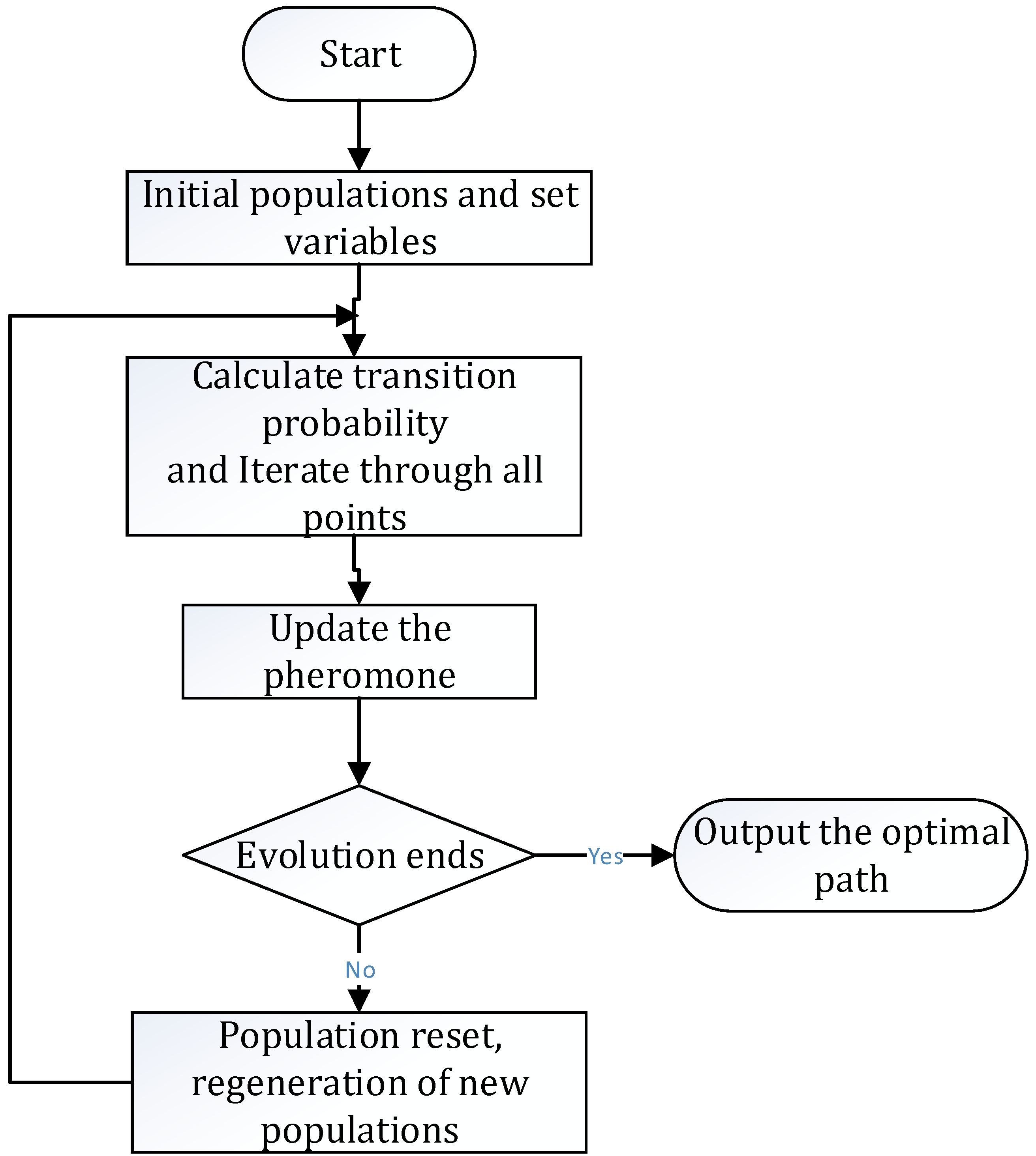
Set up multiple ants according to the specific optimization goals, and at the same time make three initial groups for the three sides of the source network load, and search separately;

(2)

Initialize an equal amount of pheromones on each path, as:

$${\tau }_{ij}(0)=C\hspace{1em}\hspace{1em}\hspace{1em}\Delta {\tau }_{ij}(0)=0$$

(29)

(3)

Take an ant, calculate the transition probability, select the next optimized calculation node according to the roulette method, and update the taboo table [16]. After each ant completes an optimized output, it releases pheromone on the path of the optimized combination. The amount of pheromone is proportional to the quality of the solution. Considering the correlation between nodes, a random local search strategy is adopted. It can optimize the operation of two adjacent nodes to the best one, and the amount of pheromone on the better node is also the largest. Later, the probability of ant selection increases;

(4)

Each ant takes the legal system node optimization path and retains the pheromone amount $\Delta {\tau }_{ij}^k$ that the ant did not release between the nodes, and the ant dies;

(5)

Repeat steps 3–4 until all ants complete the optimization process;

(6)

Compute pheromone increments $\Delta {\tau }_{ij}^k$ and pheromones for all optimization modes ${\tau }_{ij}(t+n)$;

(7)

Record this iteration path and update the current optimum combination to empty the taboo table;

(8)

Reach a predetermined number of iteration steps or stagnation (all ants choose the same path and the solution no longer changes) [17]; the algorithm ends with the current optimal solution as the optimal solution of the problem, otherwise the iteration continues.

The pheromones and transfer probabilities are modeled as follows:

(1)

Transfer probabilistic calculation formula:

$$p_{ij}^k(t)=\{\begin{array}{l}\frac{\left[\left[{\tau }_{ij}(t)\right]\right]{\left[{\eta }_{ij}(t)\right]}^{\beta }}{{{\displaystyle \sum _{s\in J_k(i)}\left[{\tau }_{is}(t)\right]}}^{\alpha }{\left[{\eta }_{is}(t)\right]}^{\beta }},if\hspace{1em}\hspace{1em}j\in J_{{}_k}(i)\\ 0,\hspace{1em}\hspace{1em}eles\end{array}$$

(30)

Inspired factor:

$${\eta }_{ij}=\frac{1}{d_{ij}}$$

(31)

where $\alpha$ and $\beta$ are two constants, representing the weighted values of pheromones and visibility, respectively.

(2)

Pheromone calculation formula:

$$\begin{array}{l}{\tau }_{ij}(t)=(1-\rho ){\tau }_{ij}+{\displaystyle \sum _{k=1}^m\Delta }{\tau }_{ij}^k\\ \Delta {\tau }_{ij}^k=\{\begin{array}{l}\frac{Q}{L_k},\hspace{1em}if ant k goes through the optimization node(i,j) in this traversal\\ 0,\hspace{1em}else\end{array}\end{array}$$

(32)

where Q is normal and L_k is all of the ants in this traversal.

(3)

Pheromone update method

$$\begin{array}{l}{\tau }_0=(n\cdot L_{nn}{)}^{-1}\\ {\tau }_i(t+1)=(1-\rho )\cdot {\tau }_i(t)+{\rho }^{,}\Delta {\tau }_i(t+1)+\epsilon (t+1),(i=1,2,3\cdots ,n)\end{array}$$

(33)

where $\rho$ is the evaporation rate, which is an additional function: $\epsilon =\mathrm{e}\Delta {\tau }_{ij}^{b,s}$.

After updating the rules, the relationship can be obtained as follows:

$$\Delta {\tau }_{ij}={\displaystyle \sum _{s\in S^m}\left[p(S^m){\displaystyle \sum _{s\in S^m|s<i,j>s}F(s)}\right]}$$

(34)

The combined problem p, which handles the transfer probability in traditional ACO, increases the difficulty of solving and uses the continuous probability distribution function instead as a solution, and the three-dimensional independent optimization result adopts the high-dimensional normal distribution, namely the multi-dimensional Gaussian function.

The multidimensional Gaussian function formula is:

$${\rm N}(x|\mu ,\Sigma )=\frac{1}{{(2\pi )}^{D/2}}\frac{1}{{|\Sigma |}^{1/2}}\exp \left\{-\frac{1}{2}{(x-\mu )}^T{\Sigma }^{-1}(x-\mu )\right\}$$

(35)

For the assumed dataset X = (x₁,…,x_n)^T, each sample is obtained independently from the Gaussian distribution using a maximum likelihood estimation method with its likelihood function of:

$$\ln p(X|\mu ,\Sigma )=-\frac{ND}{2}\ln (2\pi )-\frac{N}{2}\ln |\Sigma |-\frac{1}{2}{(x_n-\mu )}^T{\Sigma }^{-1}(x_n-\mu )$$

(36)

Using matrix derivative properties, we can obtain the Gaussian probability function to obtain the mean $\mu$ derivative form:

$$\frac{\partial }{\partial u}\ln p(X|\mu ,\Sigma )={\displaystyle \sum _{n=1}^N{\Sigma }^{-1}(x_n-\mu )}$$

(37)

With derivative $\Sigma$, the following can be obtained:

$$\begin{array}{l}\frac{\partial }{\partial u}\ln p|\Sigma |={({\Sigma }^{-1})}^T={\Sigma }^{-1}\\ \frac{\partial }{\partial {\Sigma }_{ij}}\left\{{(x_n-\mu )}^T{\Sigma }^{-1}(x_n-\mu )\right\}={(x_n-\mu )}^T\frac{\partial {\Sigma }^{-1}}{\partial {\Sigma }_{ij}}(x_n-\mu )\end{array}$$

(38)

Set up:

$$\begin{array}{l}B={\Sigma }^{-1}(x_n-\mu )\\ B^T={\left\{{\Sigma }^{-1}(x_n-\mu )\right\}}^T={(x_n-\mu )}^T{\Sigma }^{-1}\end{array}$$

(39)

Finally, the calculation is made by matrix multiplication and the following is obtained:

$$\frac{\partial }{\partial \mu }\ln p(X|\mu ,\Sigma )=-\frac{N}{2}{\Sigma }^{-1}+\frac{1}{2}{\Sigma }^{-1}\left\{{\displaystyle \sum _{n=1}^N(x_n-\mu ){(x_n-\mu )}^T}\right\}{\Sigma }^{-1}$$

(40)

Taking the multi-dimensional Gaussian ACO function, the probability density function is calculated for each step of the ant solution, and finally the complex weight combination value of multiple Gaussian functions is obtained, i.e.:

$$N_i(x|\mu ,\Sigma )={\displaystyle \sum _{k=1}^k{\omega }_k}N(x|\mu ,\Sigma )={\displaystyle \sum _{k=1}^k\frac{1}{\delta k\sqrt{2\pi }}}{e}^{-\frac{{(k-1)}^2}{2{\delta }^2{k}^2}}N(x|\mu ,\Sigma )$$

(41)

where $\delta$ is the global optimal solution computational equilibrium parameter, the smaller it is the higher the computational complexity, but the higher the probability of selecting the optimal solution. In each iteration, each ant selects a solution based on the weight in the probability density function, and N_i samples the solution through the Gaussian function, according to its covariance matrix.

For the joint scheduling optimization model in this model, there are three possible system operation states, SG(i,n), SN(i,n) and SL(i,n), representing the operating amount of the i node of the n topological island in the system. The information mainly includes the node power value, voltage value, current, and switching signal volume, and a 3D Gaussian function is used as the density function. The solution of the model is the security scheduling optimization result with the lowest joint operation cost of the ant on the topological connection path with the equilibrium node as the initial search node in any topological island.

4. Solving the Calculation Example

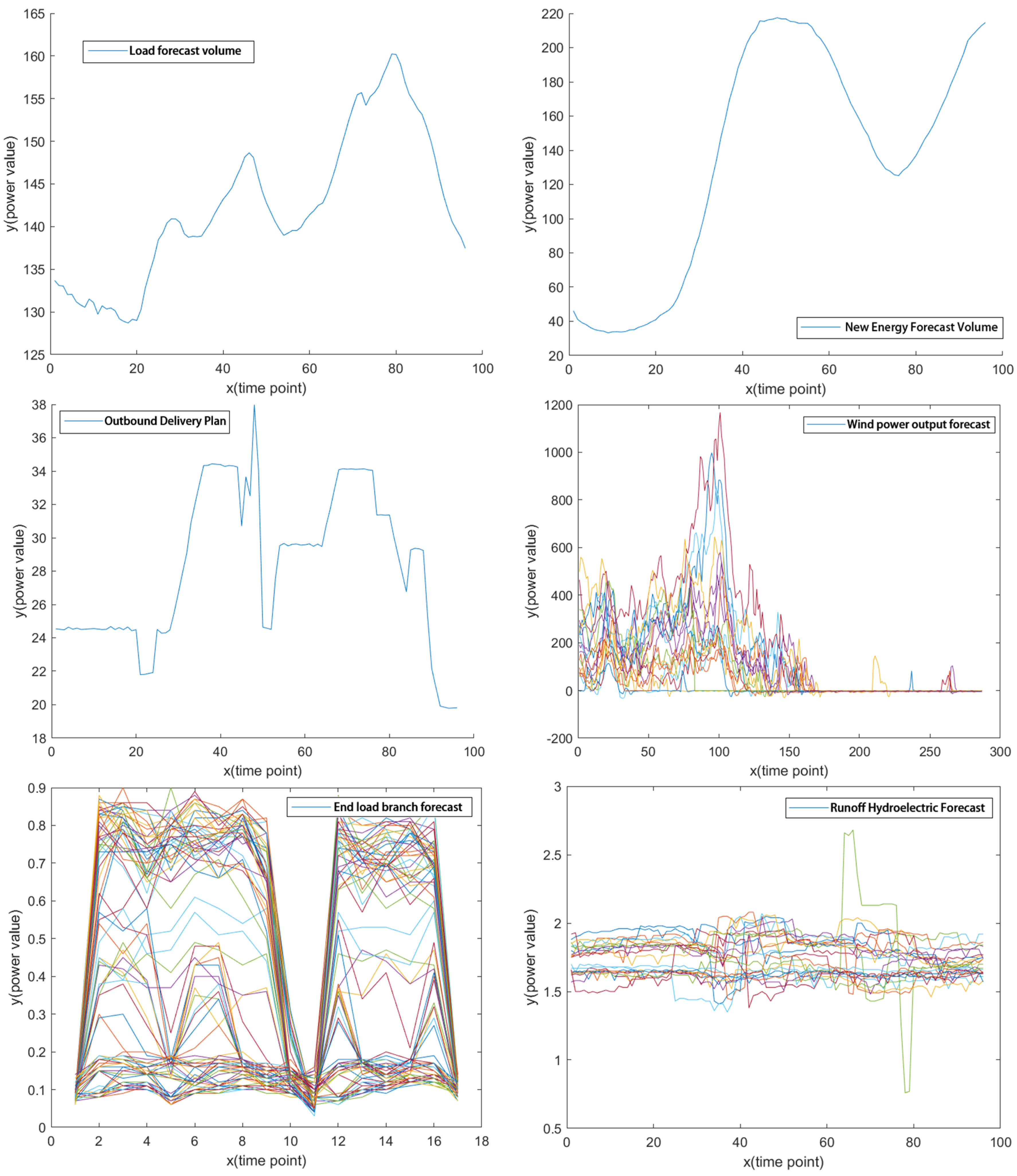
4.1. Basic Scenario

We use a simplified 36-node system structure as the main case. Due to the confidentiality needs of the power grid, the simplified node parameters are not provided temporarily [18], and the simplified topology graph is shown in Figure 2.

The 36 nodes simplified by this model are used as the basic model of distribution network calculation, including 11 independent power nodes with a total installed capacity of 270.34 MW; 16 independent load nodes with a 197.7 MW capacity for final assembly; and 9 micro-network nodes with an elastic capacity of 91.14 MW and a loading capacity of 84.63 MW. It can be seen that this distribution network is in the basic supply-and-demand balance and full delivery state.

According to this method of dividing the model, the node types within the system are shown in

Table 1. Classification of nodes in this case.

Node Number	Node Type	Response Characteristics	Main Properties	Elastic Index
1	Load	Rigid	Commercial electricity consumption	15.21%
2	Load	Rigid	Residential areas	4.36%
3	Power generation	Elasticity	Cascading hydropower	40.93%
4	Power generation	Rigid	Basin runoff is a small hydropower group	12.67%
5	Load	Rigid	Chemical plant	20.05%
6	Load	Rigid	Water works	8.32%
7	Load	Elasticity	School, energy storage	36.69%
8	Power generation	Elasticity	Wind power, energy storage	28.96%
9	Load	Rigid	Mechanical plant	9.13%
10	Load	Rigid	Food processing plant	10.14%
11	Load	Elasticity	Commercial and self-built photovoltaic energy storage	46.68%
12	Load	Rigid	Government office	31.24%
13	Power generation	Rigid	Wind force	16.21%
14	Load	Elasticity	Textile factory, belt energy storage	16.46%
15	Load	Rigid	Paper mill	8.83%
16	Power generation	Rigid	Photovoltaic power	5.49%
17	Load	Elasticity	Cotton textile mill	30.13%
18	Power generation	Rigid	Basin runoff is a small hydropower group	10.25%
19	Power generation	Elasticity	Biomass power generation	60.14%
20	Load	Rigid	Small textile mills	14.32%
21	Load	Rigid	Automobile manufacturers	10.93%
22	Load	Rigid	Energy storage battery manufacturer	4.16%
23	Load	Rigid	Steel processing plant	2.86%
24	Load	Rigid	Commercial office building	20.57%
25	Load	Elasticity	Auto parts manufacturer, PV	29.12%
26	Power generation	Elasticity	Gas-fired power generation	63.17%
27	Power generation	Elasticity	Comprehensive energy demonstration park	79.23%

.

The formed division of distribution network family groups are shown in

Table 2. Classification of families in this case.

Family Members	List of Load Nodes	List of Power Generation Nodes
1	1, 2, 7, 9, 11, 17	4, 8
2	5, 15	19
3	6, 10, 12	13, 32
4	14, 21, 23, 33, 35	36
5	20, 22, 25	18, 26, 29
6	24, 30, 31	3
7	27, 28, 34	16

, and the calculated correlation tightness matrix is too large in dimension, and thus will not be shown here.

The network contains three voltage levels, 110 kV, 35 kV, and 10 kV, Each user takes different grid voltages according to different characteristics; furthermore, each user interacts with other distribution network supply areas in the regional power grid through 110 kV. The overall supply and demand situation in the system has certain fluctuations along with the season. The supply–demand ratio is calculated by the annual monthly electricity average index. The analysis contains four dimensions: grid power, network load power, online power, and offline power, as shown in Figure 3. The relationship between the four key quantities is:

$$P_{gen}+P_{off}=P_{ld}+P_{on}$$

(42)

where $P_{gen}$ is the power generation amount, $P_{ld}$ is the load power amount, $P_{off}$ is the off-grid power amount, and $P_{on}$ is the on-grid power amount; this formula is also established for the whole grid and the power exchange of the contact line at any time.

In a historical operation situation, an auto part manufacturer burned the relevant production equipment due to high voltage in the network. The voltage of the production line data monitoring points was analyzed in Figure 4, where the average maximum daily voltage fluctuation reached 4.52%, and the maximum voltage fluctuation was 12.68%, seriously exceeding the limit. Therefore, it can be seen that the overall distribution network has had high voltage for a long time, and the terminal voltage of some generating nodes has significantly deviated from the grid-connection safety license.

4.2. Distribution Network Operation Scenario

Based on the 36-node distribution network model, the resilient node devices within it are decomposed in this paper in order to analyse the impact of the combination of security policies within each generation node. The key elastic node parameters are shown in

Table 3. Flexible node parameters.

Node Number	Node Type	Voltage Level	Main Parameters (Installed Capacity, in MW)
3	Cascading hydropower	110 kV	2 × 3.5 + 3 × 1.25 + 3 × 0.63 + 2 × 0.32 + 4 × 0.5
8	Wind farm	35 kV	16 × 2 + 1 × 1.5 + 5, Storage: 16
19	Biomass power generation	35 kV	8 × 1.5 + 4 × 3 + 3 × 5
26	Gas-fired power generation	10 kV	4 × 4.5 + 6 × 1.5
32	Photovoltaic power station	10 kV	1.2 × 5, Storage: 3.6
36	Storage capacity and power station	110 kV	6 × 4.6 + 4 × 2.5 + 8 × 1.25
7	Class II load	10 kV	Storage: 1.5. Installation capacity: 3
11	Class II load	35 kV	Light: 1.2 × 3, Storage: 2, Installed capacity: 6.3
14	Class I load	110 kV	Storage: 3.5. Installation capacity: 4.6
25	Class I load	110 kV	Light: 1 × 4, installed capacity: 7.83
27	Class II load	35 kV	Light: 1 × 14, Storage: 12, Gas: 8 × 1.5, Heat: 0.4 × 6 Installed capacity: 34
28	Class II load	35 kV	Light 1.2 × 6, Storage: 10. Pile: 10 × 0.18 + 12 × 0.035 Installed capacity: 16
30	Three types of load	10 kV	Storage: 2. Installation capacity: 2.4
34	Class II load	35 kV	Storage: 6. Installation capacity: 6.3
35	Class II load	10 kV	Storage: 3.2, Pile: 6 × 0.36 + 14 × 0.24, installed capacity: 4.2

, with the power generation ranking shown first, and the load ranking second (where 2 × 3.5 means two 3.5 MW installed units).

The overall operation curve of the whole network’s typical day is shown in Figure 5, where the relationship between the four key quantities is:

$$P_{ld}+P_{out}=P_{re}+P_{tr}$$

(43)

where $P_{out}$ is the external power, $P_{ld}$ is the load power, $P_{re}$ is the new energy power generation (including scenery power), and $P_{tr}$ is the traditional power generation (water and fire).

Initial generation input power can be seen in

Table 4. Original values of generators.

Generation Node	Active Power (MW)	Capacity (MW)
3	13.2019	15.28
4	16.6745	18.48
8	17.9025	38.5
13	6.8876	30
16	−0.066	20
18	10.5206	12.48
19	19.968	39
26	9.936	27
29	−0.1478	16
32	0.0443	6
36	40.3172	47.6

.

In the optimization analysis, each node prediction is used to superposition load predictions and power generation predictions on the full network. According to the outsourcing plan of the power grid (the 96 points of the optimization data, as shown in Figure 5), as the basic setting of the distribution network solution, new energy is designed according to the principle of priority power generation, and gas and biomass are designed as power regulation power supplies.

The first three pictures in Figure 6 show the network summary data load, power generation, and outgoing data; the last three pictures show the power generation and a single day’s predictions for the typical load of elastic users, including wind power, using a super short-term 5 min forecast for a cycle, runoff small hydropower, adopting a super short-term 15 min for a cycle, and a user, adopting a super short-term 15 min forecast for a cycle. Other users of the whole network are not detailed here.

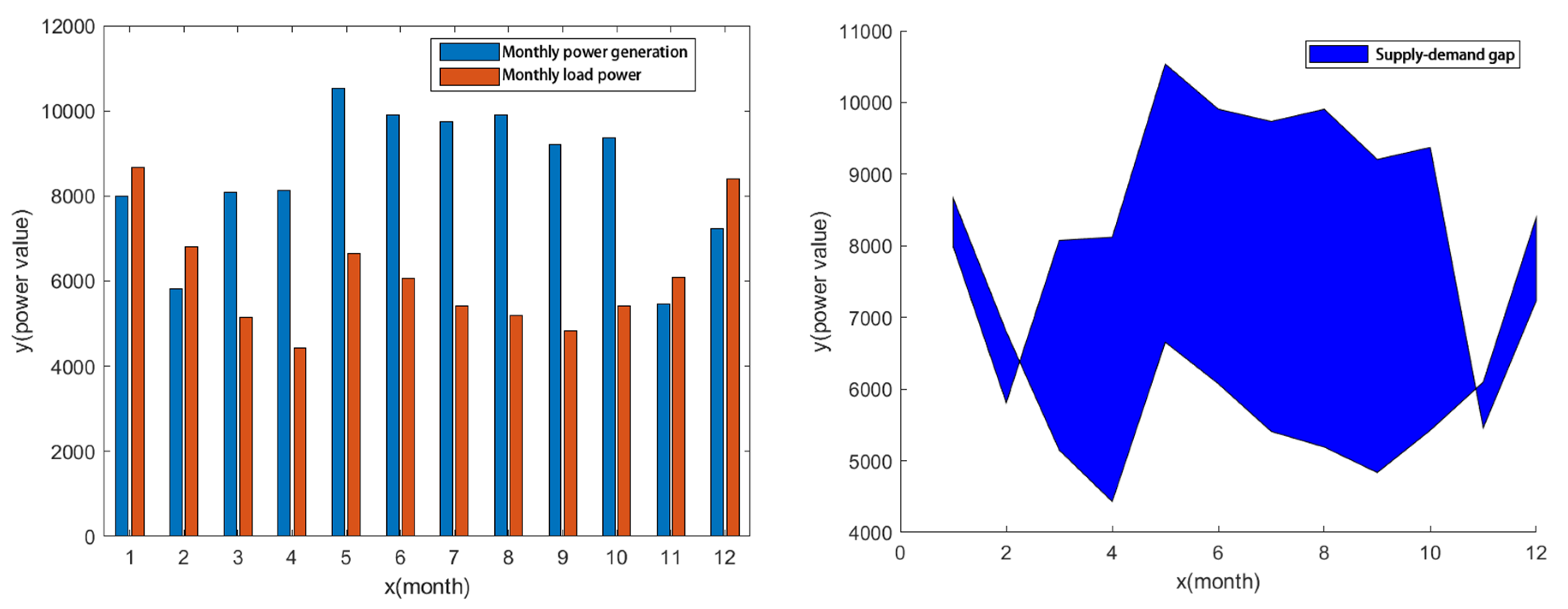
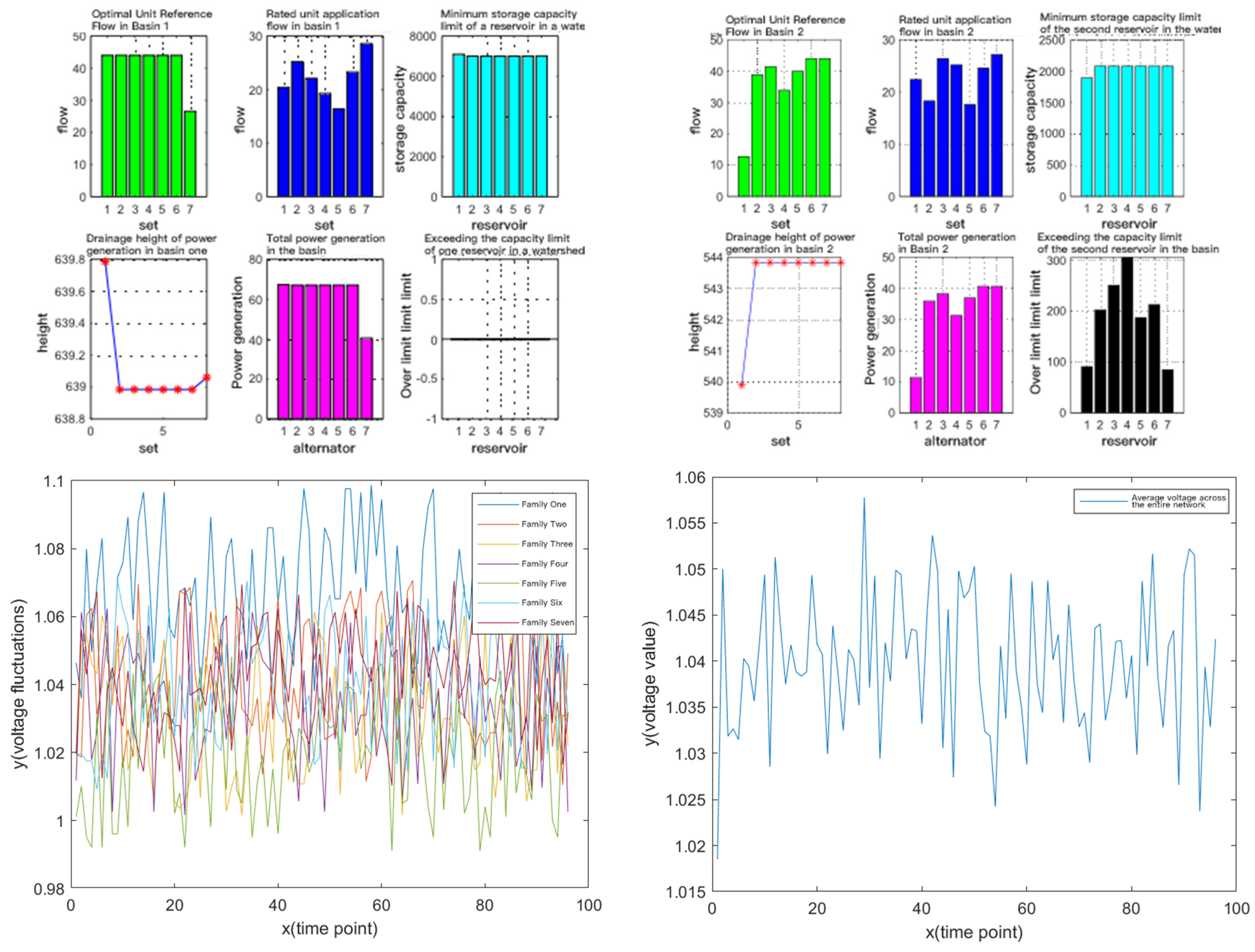
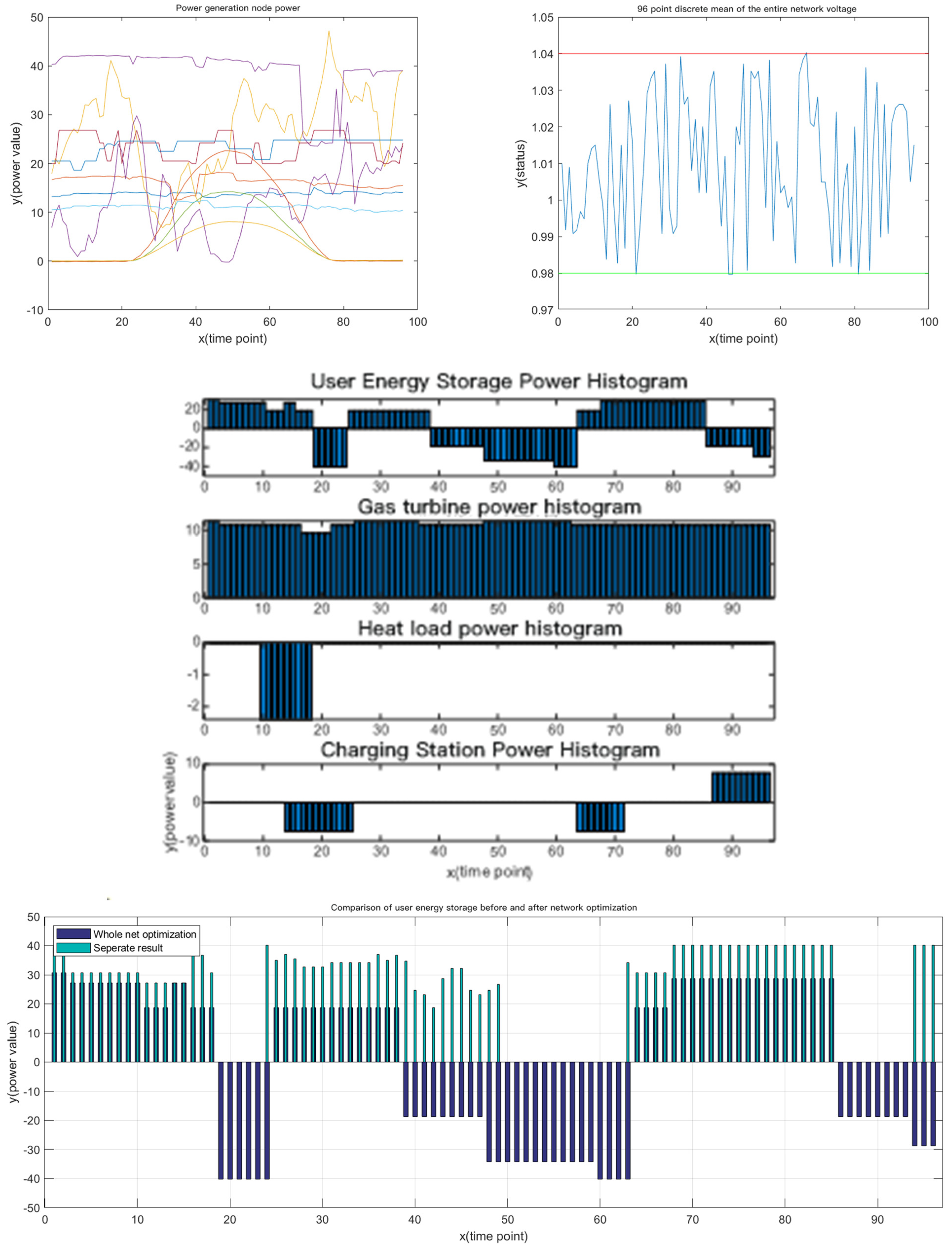
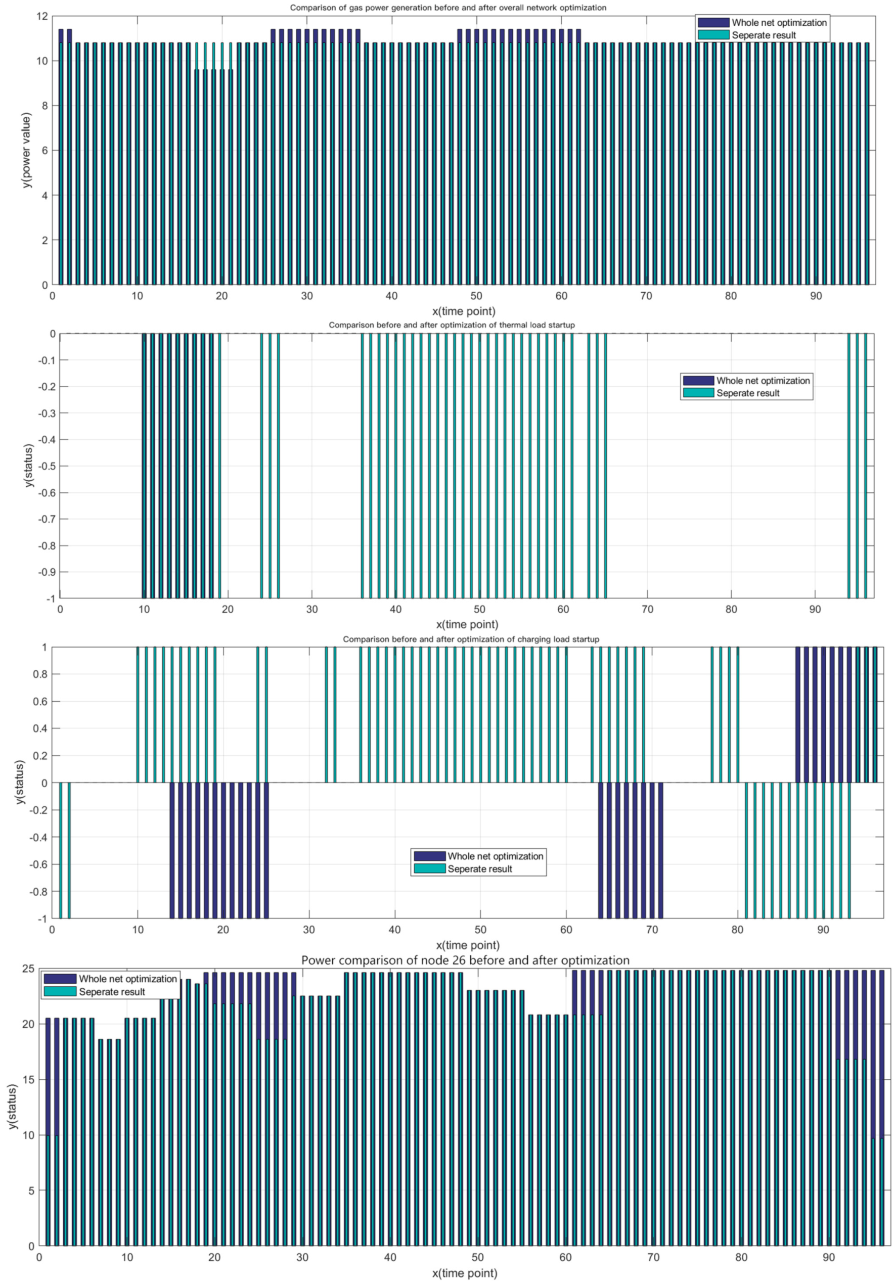
4.3. Model Calculation Results

4.3.1. Grid Voltage Control Target Value

The 96-point voltage control target of the 36-node network is shown in

Table 5. Targets of node voltage control.

Node Name	Voltage	Phase Angle	Node Name	Voltage	Phase Angle
BUS1	1	0	BUS19	1.011764051	−31.1464
BUS10	0.989535501	−19.7508	BUS20	1.011727813	−31.1951
BUS11	1.019591909	−23.7891	BUS21	1.001133166	−38.2493
BUS2	1.011749759	−31.1677	BUS26	0.991429899	−41.5284
BUS22	1.001028601	−38.277	BUS27	1	−27.8
BUS23	0.988518931	−30.1358	BUS28	1.019514092	−16.4535
BUS24	0.988722183	−30.0071	BUS29	1.01950393	−16.4518
BUS25	0.991470488	−41.5135	BUS34	1.019493038	−16.4671
BUS3	0.967180274	−41.2169	BUS4	0.991399466	−41.513
BUS51	0.994779656	−41.5325	BUS5	1.009353618	−22.8737
BUS9	0.994544278	−28.8754	BUS50	1.033333767	−31.8241
BUS12	0.990260647	−11.9921	BUS52	0.994779656	−41.5325
BUS13	1.002626092	−37.9659	BUS6	0.989535501	−19.7508
BUS14	0.998759999	−31.5197	BUS30	0.988722183	−30.0071
BUS15	1.039171437	−30.079	BUS31	1	−41.2368
BUS16	0.977696715	−20.1593	BUS33	1	−10.7673
BUS17	1.046380497	−5.50664	BUS7	1	−10.6603
BUS18	1.019633416	−23.8103	BUS8	0.989868176	−20.2014

and Figure 7, showing the voltage and phase angles of the grid at 0:00. All are displayed in unitary units.

It can be seen from the voltage control target curve that, due to the uncontrollable power supply, to ensure the system supply, the highest voltage point has been relaxed to nearly 1.07, while the minimum voltage of the whole network is about 0.95, and the overall day solution target is 0.063752189, which fully meets the voltage control target of the power grid.

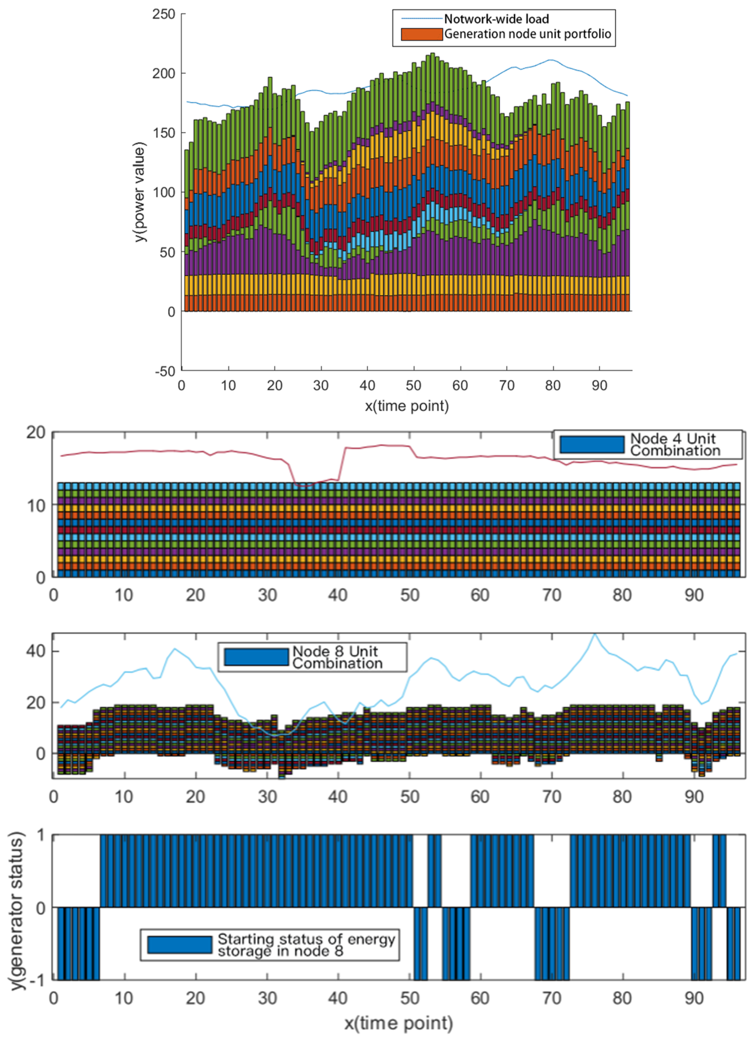
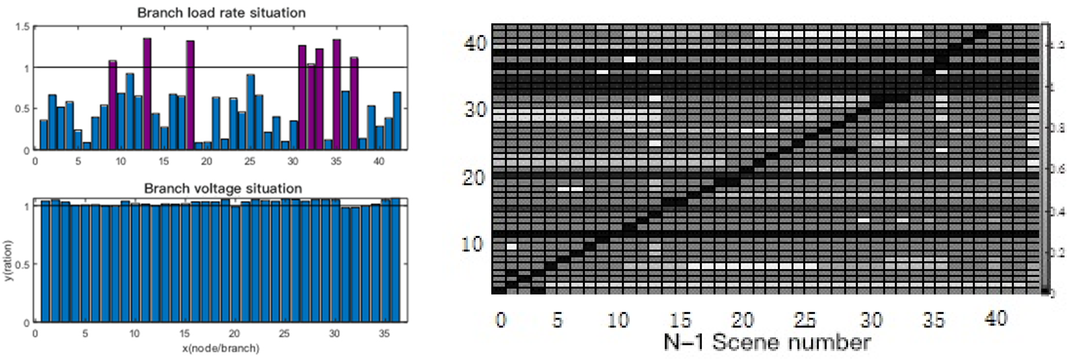
4.3.2. Optimization Result of Safety Control of Power Generation Nodes

All family combinations of units in the network are shown in Figure 7. The shutdown status identification is −1 and the boot identification is 1, to be distinguished by the line of x = 0.

In Figure 8, the first figure shows the output curve at the same time to show the cascade scheduling combination and the voltage fluctuation diagram under the combination of each family unit.

The analysis of each relevant unit combination is as follows:

The role of energy storage in the power generation unit can be intuitively displayed from the diagram, especially with wind power and photovoltaic outputs, as a power regulation device with a high enabling frequency, which can effectively make up for the characteristics of scenery fluctuations;

Nodes 4, 16, 18, and 29 are connected with unadjustable hydropower and photovoltaic power; of these, photovoltaic power has reactive compensation, so all start-up strategies are adopted. Because the families in which the small hydropower is located all have other adjustable power sources, the results for the small hydropower are all units fully open, the same as for node 4;

Nodes 19 and 26 are high-controllable generator sets, and the basic unit combination strategies are the same. It can be found from the unit combinations that the combination of power outputs is not the minimum open number combination completed by the algebraic superposition mode;

The optimization combination strategy of a storage capacity adjustable hydropower unit is relatively complex. Since most of them are cascading hydropower combination models with storage capacity plus runoff, the active and reactive situation of their overall outputs and the utilization of water conservancy resources should be considered. Therefore, adopt all power-up strategies for cascading hydropower to limit the power generation and drainage to achieve the voltage control target;

Under the reactive control of the combined voltage of independent units, the time limit of current trend analysis will occur even with the target constraints. In particular, the randomness of the hydropower + wind power combination is always high, resulting from the reactive output of two types of units. Therefore, it is seen that the reactive control of an ADN cannot completely rely on the power generation side, and requires the coordination of load-side and power grid reactive devices.

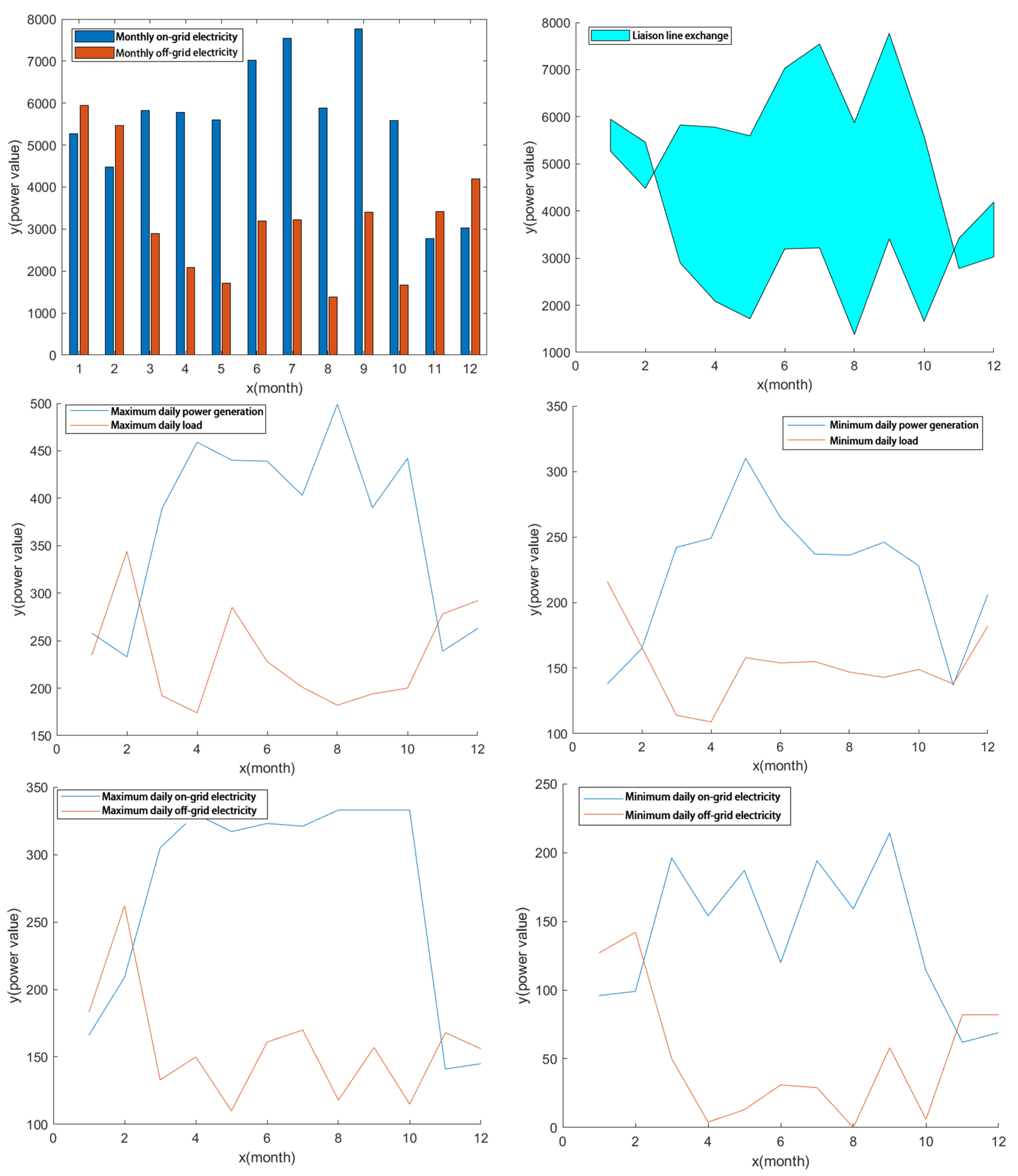
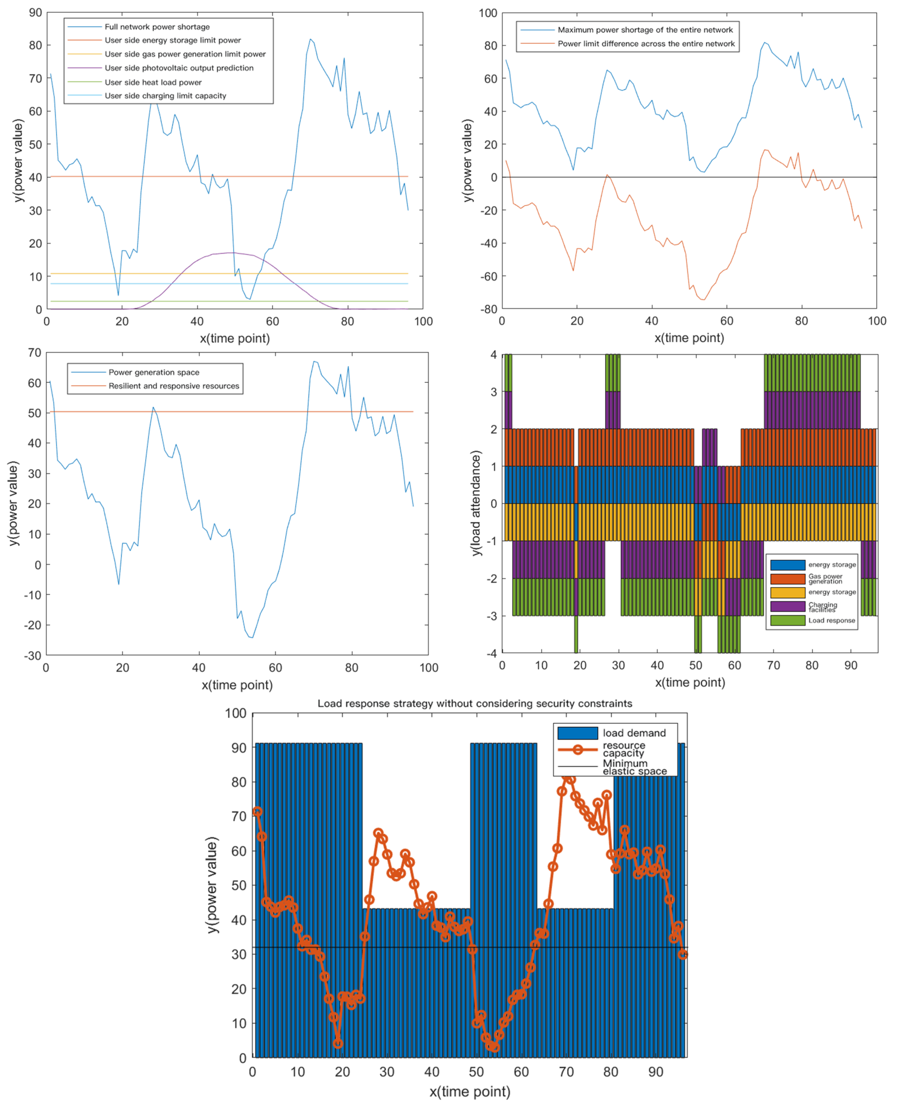
4.3.3. Optimization Result of Load Node Safety Control

The virtual power generation combination of whole network load flexible resources in the ideal state is shown in Figure 9; this is the output result under the unified adjustment mode of the whole network load, which is not consistent with the actual output according to family status, as shown in Figure 10. It is obvious that the number of load nodes involved is more than in the ideal state.

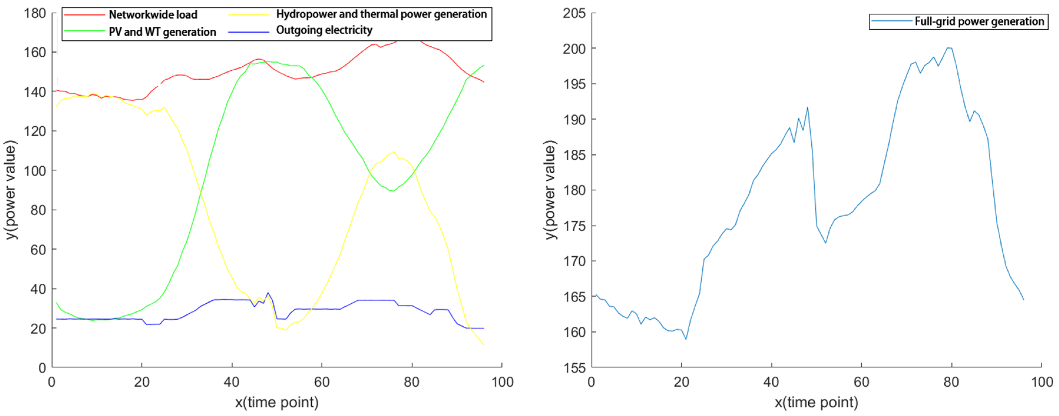
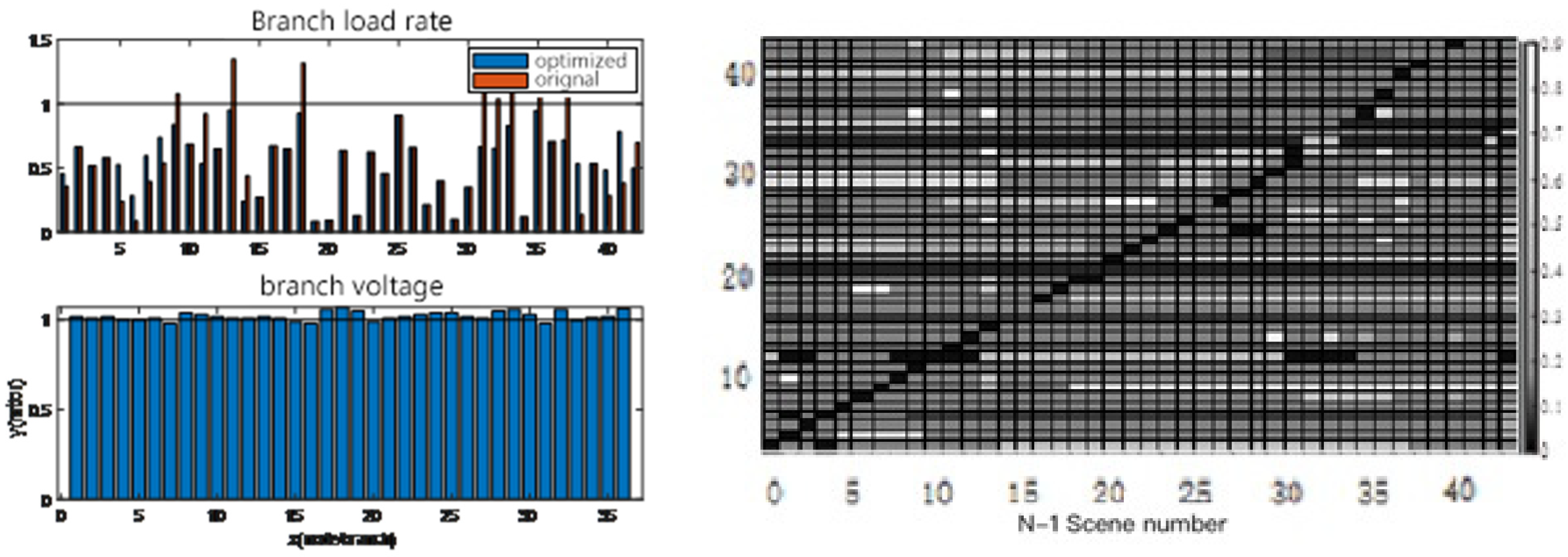
4.3.4. Combined Optimization

According to the combination of nodes, the initial point section, and the N-1 safety analysis, we obtained the results shown in Figure 11; N-1 shows the N-1 scene number and the vertical coordinates and the gray scale indicates the load rate of each branch in different N-1 scenarios. The overall visible voltage control condition is good between 0.98 and 1.07, but there is a serious branch limit. The most serious branch, 13, reaches 1.349, and cannot meet the system safety operation requirements.

The initial point current flow and N-1 safety analysis after the ant colony optimization whole network solution is shown in Figure 12. When the voltage is in a stable state, the overload problem is completely eliminated and meets the operational requirements of the power grid to optimize the load; the maximum branch load is 0.9487. There is still some room for optimization. The overall joint optimization results solved by the heuristic algorithm are shown in Figure 13.

After the optimization and solution of the whole network, the new energy combination of the power generation nodes has not changed. Node 26 is readjusted, and the user-side energy storage devices, heat load, and charging piles are adjusted greatly. Combined with the maximum load response elastic space, the power exchange is adjusted to meet the balance of supply and demand in the network and ensure the maximum demand response value.

The above calculation example’s analysis is as follows:

With the maximum load of 96 points, N-1 is 0.9621. After multiple optimizations and iterative solutions, it is found that the calculation has reached the current optimal value, and the equipment transformation should be conducted for this branch;

The whole network voltage is maintained between 0.98 and 1.04, with good results. The number of changes in the optimization of the power generation combinations is small, mainly because it is the power output end, and the appropriate increase in the reactive compensation devices on the power grid side and the user side is helpful to further stabilize the whole network voltage;

The installed capacity and the inverter power determine the actual start-stop state, which may be quite different from the theoretical calculation;

The independent power supply family in an ADN is about equal to 0 with current technology, especially the distribution grids that rely mainly upon new energy, which needs to be adjusted by conventional power supplies, energy storage, contact lines, etc.

5. Conclusions

This paper mainly analyzes an interactive model of source network load scheduling optimization with operational safety as the main goal. In the safety optimization analysis, considering the different operating characteristics of the distribution network and the transmission network, the method of joint optimization after independent analyses and calculations of the source network and the loads on the three sides is adopted.

(1)

For power generation nodes, the mode of source-source interaction is adopted, the unit combination mode of the output node is considered, the safety control model of the power generation node is constructed, and the operating boundary conditions of the generator set are used as constraints to obtain the operating safety combination of the units in the network.

(2)

For the load node, this paper uses a flexible control model to calculate and analyze the safety scheduling strategy of the load; the model of node voltage deviation in one day is used as the ultimate objective function to solve the safety scheduling of the distribution network. After calculating the independent safety scheduling model, a joint optimization model is established according to a heuristic algorithm model to analyze the overall network security characteristics of the active distribution network, and a Lagrangian relaxation calculation is introduced to ensure that the optimization target is obtained in the active distribution network.

(3)

The model availability and accuracy of this section are verified through the actual grid calculation examples, and it is found via the actual comparison that the power quality in the network can be effectively optimized and adapted to the optimization analysis of the active distribution grid of various new energy scenarios.

(4)

The overall safety requirements of the source–network–load interaction, especially voltage stability, are the basis for ensuring that the source–network–load interaction can be implemented. Good distribution network planning and internal family division of the distribution network can maximize the internal reliability indicators of the distribution network. Therefore, in the design and planning of the new ADNs, a good family analysis is required. Some current grid plans can already meet this demand to a great extent.

However, this article does not consider distribution network scheduling optimization strategies in the context of AC–DC hybrid distribution networks, electric vehicles, or large-scale energy storage applications. From the overall optimization principle, the scheduling unit of the distribution network family can be further refined. It has some similarities with current load agents, microgrids, etc., but its operating mechanism and scheduling mechanism are better. Taking the family as the basic scheduling unit is more conducive to optimization analysis and calculation of the plug-and-play distribution network. There is no need to consider the characteristics of the access node too much, as it will increase the complexity of the model. Therefore, the model of the internal family division of distribution networks should be an important research direction for the optimization and analysis of the scheduling of active distribution networks.

References

1. Jiayi, H.; Chuanwen, J.; Rong, X. A review on distributed energy resources and MicroGrid. Renew. Sustain. Energy Rev. 2008, 12, 2472–2483. [Google Scholar] [CrossRef]
2. Ehsan, A.; Yang, Q. State-of-the-art techniques for modelling of uncertainties in active distribution network planning: A review. Appl. Energy 2019, 239, 1509–1523. [Google Scholar] [CrossRef]
3. ALKaabi, S.S.; Zeineldin, H.H.; Member, S.; Khadkikar, V. Planning active distributionnetworks considering multi-DG configurations. IEEE Trans. Power Syst. 2014, 29, 785–793. [Google Scholar] [CrossRef]
4. Xing, H.; Cheng, H.; Zhang, Y.; Zeng, P. Active distribution network expansion planningintegrating dispersed energy storage systems. IET Gener. Transm Distrib. 2016, 10, 638–644. [Google Scholar] [CrossRef]
5. Mashayekh, S.; Stadler, M.; Cardoso, G.; Heleno, M.; Madathil, S.C.; Nagarajan, H.; Bent, R.; Mueller-Stoffels, M.; Lu, X.; Wang, J. Security-constrained design of isolated multi-energy microgrids. IEEE Trans. Power Syst. 2018, 33, 2452–2462. [Google Scholar] [CrossRef]
6. Koltsaklis, N.E.; Kopanos, G.M.; Georgiadis, M.C. Design and operational planning of energy networks based on combined heat and power units. Ind. Eng. Chem. Res. 2014, 53, 16905–16923. [Google Scholar] [CrossRef]
7. Perković, L.; Mikulčić, H.; Pavlinek, L.; Wang, X.; Vujanović, M.; Tan, H.; Baleta, J.; Duić, N. Coupling of cleaner production with a day-ahead electricity market: A hypothetical case study. J. Clean. Prod. 2017, 143, 1011–1020. [Google Scholar] [CrossRef]
8. Kumar, S.; Sushama, M. Sushama, Strategic demand response framework for energy management in distribution system based on network loss sensitivity. Energy Environ. 2020, 31, 1385–1402. [Google Scholar] [CrossRef]
9. Tan, W.-S.; Hassan, M.Y.; Majid, M.S.; Abdul Rahman, H. Optimal distributed renewable generation planning: A review of diferent approaches. Renew. Sustain. Energy Rev. 2013, 18, 626–645. [Google Scholar] [CrossRef]
10. Santos, S.F.; Fitiwi, D.Z.; Bizuayehu, A.W.; Shafie-khah, M.; Asensio, M.; Contreras, J.; Cabrita, C.M.; Catalão, J.P. Novel multi-stage stochastic DG investment planning with recourse. IEEE Trans. Sustain. Energy 2016, 8, 164–178. [Google Scholar] [CrossRef]
11. Yang, Q.; Barria, J.A.; Green, T.C. Communication infrastructures for distributed control of power distribution networks. IEEE Trans. Ind. Inform. 2011, 7, 316–327. [Google Scholar] [CrossRef]
12. Ehsan, A.; Yang, Q.; Cheng, M. A scenario-based robust investment planning model for multi-type distributed generation under uncertainties. IET Gener. Transm. Distrib. 2018, 12, 4426–4434. [Google Scholar] [CrossRef]
13. Billinton, R.; Allan, R.N. Reliability Evaluation of Power Systems; Springer Science & Business Media: Boston, MA, USA, 2013. [Google Scholar]
14. Heidari, A.; Agelidis, V.G.; Kia, M.; Pou, J.; Aghaei, J.; Shafie-Khah, M.; Catalão, J.P. Reliability optimization of automated distribution networks with probability customer interruption cost model in the presence of dg units’. IEEE Trans. Smart Grid. 2017, 8, 305–315. [Google Scholar]
15. Niknam, T.; Kavousifard, A.; Aghaei, J. Scenario-based multiobjective distribution feeder reconfiguration considering wind power using adaptive modified particle swarm optimization. IET Renew. Power Gener. 2012, 6, 236–247. [Google Scholar] [CrossRef]
16. Ghadi, M.J.; Ghavidel, S.; Rajabi, A.; Azizivahed, A.; Li, L.; Zhang, J. A review on economic and technical operation of active distribution systems. Renew. Sustain. Energy Rev. 2019, 104, 38–53. [Google Scholar] [CrossRef]
17. Li, Y.; Yang, Z.; Li, G.; Mu, Y.; Zhao, D.; Chen, C.; Shen, B. Optimal scheduling of isolated microgrid with an electric vehicle battery swapping station in multi-stakeholder scenarios: A bi-level programming approach via real-time pricing. Appl. Energy 2018, 232, 54–68. [Google Scholar] [CrossRef]
18. Mahmood, S.A.; Zedan, M.J.M. Network Load Balancing in Teleconferencing Systems. In Proceedings of the 2022 8th International Engineering Conference on Sustainable Technology and Development (IEC), Erbil, Iraq, 23–24 February 2023; pp. 12–16. [Google Scholar]
19. Kyriakou, D.G.; Kanellos, F.D. Optimal operation of microgrids comprising large building prosumers and plug-in electric vehicles integrated into active distribution networks. Energies 2022, 15, 6182. [Google Scholar] [CrossRef]
20. Weishan, D.; Yongjuan, L. Research on grid-connected distributed power grids based on solar power generation systems. Power Technol. 2017, 1052–1054. [Google Scholar]
21. Li, Y.; Wei, X.; Li, Y.; Dong, Z.; Shahidehpour, M. Detection of false data injection attacks in smart grid: A secure federated deep learning approach. IEEE Trans. Smart Grid 2022, 13, 4862–4872. [Google Scholar] [CrossRef]
22. Siwu, L.; Sichang, X.; Fangmei, B.; Yulin, Y.; Xiaodi, M.; Chan, P. The analysis of business scenarios and implementation path of “5G+ Source-network-load-storage” multi-station integration. E3S Web Conf. 2021, 248, 02031. [Google Scholar]
23. Li, Y.; Feng, B.; Wang, B.; Sun, S. Joint planning of distributed generations and energy storage in active distribution networks: A Bi-Level programming approach. Energy 2022, 245, 123226. [Google Scholar] [CrossRef]
24. Fan, H.; Yu, Z.; Xia, S.; Li, X. Review on coordinated planning of source-network-load-storage for integrated energy systems. Front. Energy Res. 2021, 9, 641158. [Google Scholar] [CrossRef]
25. Chen, X.U.E.; Jing, R.E.N.; Zhang, X.; Wang, P.; Zhou, X.; Liu, Y.; Kuang, H. An optimal dispatch method for high proportion new energy power grid based on source-network-load-storage interaction. In Proceedings of the 2021 4th International Conference on Electron Device and Mechanical Engineering (ICEDME), Guangzhou, China, 19–21 March 2021; pp. 119–122. [Google Scholar]
26. Li, Y.; Zhang, M.; Chen, C. A deep-learning intelligent system incorporating data augmentation for short-term voltage stability assessment of power systems. Appl. Energy 2022, 308, 118347. [Google Scholar] [CrossRef]
27. Xu, R.; Chen, C.; Chen, D.; Zhou, G.; Jin, Y.; Wu, X.; Lin, Z. Maximum openable capacity optimization method of active distribution network considering multiple users access. Energy Rep. 2022, 8, 43–50. [Google Scholar] [CrossRef]
28. Piao, Z.; Peng, T.; Lu, S.; Zhang, Y.; Cheng, D.; Wang, J. Efficient collaborative utilization mode of “Source-network-load-storage” to improve energy-self-balance ability of microgrid. In Proceedings of the 2022 4th International Conference on Power and Energy Technology (ICPET), Beijing, China, 28–31 July 2022; pp. 498–503. [Google Scholar]
29. Li, Y.; Yang, Z.; Li, G.; Zhao, D.; Tian, W. Optimal scheduling of an isolated microgrid with battery storage considering load and renewable generation uncertainties. IEEE Trans. Ind. Electron. 2019, 66, 1565–1575. [Google Scholar] [CrossRef]
30. Wang, J.; Huo, S.; Yan, R.; Cui, Z. Leveraging heat accumulation of district heating network to improve performances of integrated energy system under source-load uncertainties. Energy 2022, 252, 124002. [Google Scholar] [CrossRef]
Figure 1. Basic solution process of ACO.
Wevj 14 00159 g001
Figure 2. 36-node active distribution network structure diagram.
Wevj 14 00159 g002
Figure 3. The 36-node grid characteristic analyses.
Wevj 14 00159 g003aWevj 14 00159 g003b
Figure 4. Voltage fluctuation situations of a special user.
Wevj 14 00159 g004
Figure 5. The whole net power curve of a typical day.
Wevj 14 00159 g005
Figure 6. The 96 data points for a day’s optimization. Each color in the figure represents the predicted terminal load of different branches.
Wevj 14 00159 g006
Figure 7. Targets of voltage control for the grid. Each color in the figure represents the voltage of a different node.
Wevj 14 00159 g007
Figure 8. Generator combinations of the network. Each color in the figure represents the output power of different units.
Wevj 14 00159 g008aWevj 14 00159 g008bWevj 14 00159 g008c
Figure 9. Load response combinations of the ideal state.
Wevj 14 00159 g009
Figure 10. Load response combinations of safe strategies.
Wevj 14 00159 g010aWevj 14 00159 g010b
Figure 11. Original combination safety check results. Each color in the figure represents different branches.
Wevj 14 00159 g011
Figure 12. Optimization of union calculation results.
Wevj 14 00159 g012
Figure 13. Comparison of the starting state of each node before and after optimization.
Wevj 14 00159 g013aWevj 14 00159 g013bWevj 14 00159 g013cWevj 14 00159 g013d