An Electric Bus Battery Swapping Station Location Method Based on Global Optimized Peak Traffic Flow

Abstract

The electric bus is an extremely important part of urban public transportation and has a huge impact on the ecosystem. However, the battery capacity is still a tough problem, and electric buses often face a booming demand for charging during peak periods. This paper focuses on the problem of electric bus battery swapping station (BSS) location. Based on the traffic flow assignment theory, this paper proposes a hybrid traffic assignment method based on GA and Frank–Wolfe algorithm, which has proved to be closer to the global optimum than the traditional method. This paper proposes a BSS selection model considering service quality as an evaluating indicator and a simulation is made based on a virtual road network. Compared with the traditional method, the result from the hybrid method is more suitable for electric buses when considering the situation at peak hours.

1. Introduction

The transportation sector, as a major contributor to greenhouse gas emissions, is under pressure to meet energy conservation and reduction goals. Public bus systems are an essential part of the transportation environment, offering passengers an affordable and eco-friendly travel option while also playing a crucial role in easing traffic congestion and decreasing exhaust emissions [1]. Due to the advantages associated with emission reduction and fuel efficiency improvement, battery-powered electric buses are considered to be a promising alternative to conventional diesel buses [2]. One of the key questions of electric bus use is selection of charging station locations. The location of the charging station can have a significant impact on its effectiveness and efficiency.

Previous studies on charging station locating mainly focused on the interaction between electric bus charging stations and distribution facilities, aiming to minimize the charging cost, including both electricity demand charges and energy charges. Dan and Ban [3] present a mixed-integer linear programming model that optimizes the trade-off between upfront charging infrastructure costs and operational performance. He et al. [4] propose a network modeling framework to optimize charging for a fast-charging BEB system, minimizing costs. The problem is initially formulated as a nonlinear non-convex program with continuous variables. A discretized method and reformulation technique are used to transform the model into a linear program, easily solvable even for large-scale problems. Oier et al. [5] present a standardized framework for micro-scale analysis of potential electric bus charging locations tailored to Stockholm. To promote expansion, the framework is identifying connecting charging stations to the power grid as the main problem point in city-center locations and accounting for up to 63% of the total cost. Azadeh et al. [6] evaluate the cost of electrifying an existing bus network using a family of bi-objective mathematical models. These models assess the trade-off between strategic decisions (battery sizing and charging station locations) and operational decisions (battery degradation) by investigating various charging policies. Flexible energy loss policies can result in up to 17% savings in battery aging for a Rotterdam bus network. Tugce and Onur [7] propose a MILP model for location and capacity decisions of EBCSs to ensure road network connectivity in a region. Routes, demand and driving ranges of electric buses are considered to determine locations and capacities under waiting time constraints. The model observed that driving ranges have the highest importance in the efficient use of electric buses, and that charging durations, number of trips and service rates significantly affect capacities of stations. Dionysios et al. [8] developed a model for optimally locating the charging station in an electric bus network, considering bus queuing delays. An integer linear programming model minimizes investment costs for deploying opportunity charging facilities. An M/M/1 queuing model incorporates bus queuing considerations at terminal charging locations. Li et el. [9] point out that for e-bus fleets with small battery capacity and short recharge time, a unified charging strategy cannot extend battery life, reduce operating costs or ensure punctuality due to varying charging time and energy usage. A personalized charging strategy using genetic and nearest neighbor algorithms was proposed, utilizing time-varying constraints and a penalty function.

Recently, there has been a great deal of interest in battery swapping stations (BSS), particularly in China. Electric vehicles and rechargeable batteries have always been treated as a unified whole in traditional thinking. However, the difference of user distributed decision making leads to the obvious characteristics of mobility, dispersion of charging and randomness of connecting to the power grid, which causes many uncertain impacts and influences on the distribution network. Unlike charging methods, BSS deployment is more versatile and requires only a few minutes for charging. In fact, the number of battery-swapping vehicles sold in China has exceeded 160,000, with a year-on-year growth of 162% and a market penetration rate of 4.6% in 2021 alone. Furthermore, there are currently over 1600 BSSs in operation. It is projected that by 2025, the sales of battery swapping vehicles and number of BSSs in China will surpass 1.92 million and 30,000, respectively [10]. Zhang and Chen [11] explore the feasibility of direct power trading in the charging and swapping market by comparing BCSS’s economic benefits under three power purchase models. The results show that the direct power trading model can significantly increase the project’s NPV and IRR, making up for investment costs. Wang and Hou [12] present a real-time optimization strategy for recommending an optimal station for the EV upon its swapping request. In this strategy, rolling optimization and Lyapunov optimization from two different time scales are combined, saving the EV owners’ time lost due to swapping, while improving the operational economy and stability of battery swapping stations and the distribution network. Lu et al. [13] propose a shared charging and switching station model under the “centralized charging and unified distribution” model, in which centralized charging stations are built in suburban areas, and switching stations are built in urban areas. This model allows horizontal transfer between switching stations and establishes corresponding site selection decision guidelines. Zhao et el. [14] present a Distributionally Robust Optimization model for day-ahead dispatch of a novel battery charging and swapping station. The model is reformulated as a tractable MILP using affine decision rules. Case studies demonstrate that charging/discharging freedom enhances operational flexibility and reduces 22.9% of total cost.

The research above mainly focuses on the marketization and daily operation of the BSSs. Not many studies focus on the location problem of the battery swapping station. Wang et al. [15] developed a model for selecting battery swapping station locations that utilizes the multi-criteria decision making (MCDM) method and incorporates three evaluation criteria: economic, technical and social impact. Huang and Kockelman [16], on the other hand, focus on maximizing profits by taking into account elastic demand, station congestion and network equilibrium, using a genetic algorithm to identify optimal charging station locations. Ren et al. [17] utilize a combination of the grey decision model and genetic algorithm to minimize the total cost of charging stations, ultimately determining the optimal position for these stations. Zu and Sun [18] consider BSS as a complex task that involves multiple objectives, such as minimizing total cost, maximizing user satisfaction and reducing energy consumption, and present a planning model for site selection that takes into account user behavior and uses the YALMIP/CPLEX method to solve the problem.

As an infrastructure, the electric bus needs to have a BSS for charging and replacing batteries. According to the literature above, it can be concluded that existing research on the BSS location problem mainly focuses on the field of electric cars, and most research chooses energy cost and user satisfaction as a major consideration. For electric cars, energy costs are truly an important factor, but focusing on energy costs does not apply to public transport systems. Because of the public welfare attribute of public transport, when considering the location of public transport facilities, service quality of the system is more significant than the total consumption. Traffic flow has great influence on the operation situation of electric buses. Therefore, it is necessary to choose the location of the BSSs according to convenience and accessibility, and to not let the buses detour or stay for too long. Road width, bus frequency and other factors will also affect the congestion and operation mode of electric buses. Based on the global optimal traffic flow assignment algorithm, this paper mainly considers the influence of road flow and congestion on the location of the BSSs, establishing and optimizing the model, and finally obtains the location reference.

The structure of this paper is as follows:

Section 1 introduces the background and current research status both domestically and internationally.

Section 2 is methodology, which presents the GA-FW algorithm used for traffic flow optimization and an improved GA algorithm used for location model optimization.

Section 3 is the model introduction. Based on traffic flow theory, this paper establishes an electric bus driving and BSS location model. A road network and bus operation system model are built specifically for the selected area in Beijing.

Section 4 presents the result and analysis of the traffic assignment and BSS location model.

The conclusion section is a summary of the work above and the application value of this research. This section also addresses the limitations of this study and provides the direction for future research.

2. Methodology

2.1. Frank–Wolfe Method

The Frank–Wolfe method is a traditional dynamic traffic assignment algorithm that employs a step-by-step linear programming approach to nonlinear programming. It comprises two primary components: determining the search direction in each iteration and determining the search step size. The optimal step size in the direction of the quickest descent is used to intercept the starting point of the next iteration. Throughout each iteration, the all-or-nothing method is employed for allocation to obtain the iteration direction, and the step size of each iteration is calculated through dichotomy. The flow of all road sections is continuously looped until the optimal solution is attained. This approach is only viable when the model constraints are linear as the solution of the linear programming problem must be solved at each iteration. It is not suitable for general linear programming models due to the high computational burden. Hence, this method is solely applicable when the approximate programming model is easy to solve, which is the hallmark of traffic assignment.

The function of the Frank–Wolfe method to achieve traffic assignment can be described as:

$$f=\sum _{\left(i,j\in A\right)}{\int }_0^{\eta x_{ij}^{hat}+\left(1-\eta \right)x_{ij}}{t}_{ij}\left(\omega \right)d\omega$$

(1)

The optimal step size can be calculated by:

$$f\frac{df}{d\eta }=0$$

(2)

$$\Rightarrow \frac{d}{d\eta }\sum _{\left(i,j\in A\right)}{\int }_0^{\eta x_{ij}^{hat}+\left(1-\eta \right)x_{ij}}{t}_{ij}\left(\omega \right)d\omega =0$$

(3)

$$\Rightarrow \sum _{\left(i,j\in A\right)}{t}_{ij}\left({\eta x}_{ij}^{hat}+\left(1-\eta \right)x_{ij}\right)\left(x_{ij}^{hat}-x_{ij}\right)=0$$

(4)

2.2. Modified Genetic Algorithm

In this paper, the classic genetic algorithm (GA) is used as the optimization algorithm in the traffic assignment model, and a modified GA is applied for the BSS location model. The following describes the variables and the setting methods of the modified GA for the BSS location model.

(1)

Individual.

The individual in the genetic algorithm is set to dimension degree is equal to the vector $N_{bs}$ × 1, where $N_{bs}$ is the bus constructed by the location model, the total number of bus stations within all bus routes in the operating system. Each element within an individual has 0–1 value, in which 0 indicates that there is no BSS in the area around the corresponding bus station and 1 indicates that there is a BSS in the area around the corresponding bus station. Each individual represents a site-selection scheme, indicating the selection status of all potential BSSs in the region. In a single entity, one element can only represent one bus station.

(2)

Optimization constraints.

The constraint on the location of the BSSs is that in the electric bus driving simulation, when a bus is driving into a BSS, the remaining battery capacity cannot be under a safe level. The setting method of constraint is to add a penalty item. When the remaining capacity is under the safe level, a maximum value is added to the fitness function.

(3)

Fitness.

In a genetic algorithm, fitness is used to reflect the degree of the individual’s adaptation and satisfaction to the optimization goal. In this paper, the fitness of each individual is set to be the sum of equivalent distances of all selected stations. For this reason, the lower the fitness of the individual, the more satisfied the optimization goal.

(4)

Selection.

The roulette selection method is used to select the parent individual to generate the offspring according to the fitness of all individuals in the population.

(5)

Crossing.

A uniform crossing method is adopted in which two fragments with the same random length are randomly selected within the range of individuals. Then, the fragments within the crossing range are exchanged.

(6)

Mutation.

In this paper, 3 mutation modes are set up. Mutation mode 1: the selected state of one station is exchanged with the state of another station. Mutation mode 2: randomly select a not selected station on an individual. Mutation mode 3: randomly change the selected state of a station. If the element is 1, it becomes 0; if it is 0, it becomes 1.

2.3. Traffic Flow Assignment Based on GA-FW Method

The objective function is selected to minimize the total impedance. A path searching algorithm based on GA-FW hybrid algorithm is used to solve the problem. The specific steps are as follows, and the process is shown in Figure 1:

Step 1: Initialization

(1) Road network parameters: the number of nodes, the number of road segments, the demand of each OD point pair, distance between nodes, road level information, road capacity, road design speed.

(2) Genetic algorithm parameters: number of populations, minimum number of iterations, maximum number of iterations, crossover probability, mutation probability, etc.

Step 2: According to the path search algorithm, find the top K paths between OD points and store the data information in the form of a path-section matrix.

Step 3: According to the encoding form, randomly generate M pending solutions and calculate corresponding values.

Step 4: According to the fitness function, calculate the fitness.

Step 5: Consider whether the termination condition of genetic algorithm is satisfied. If it is satisfied, terminate the iteration and output the current optimal solution and go to Step 7. If not, go to Step 6.

Step 6: Retain the first 30% of the good individuals of the current generation, eliminate the last 20% of the poor individuals, and the remaining individuals enter the transmission through the roulette wheel method for the next step of selection, crossover, mutation. Keep the overall population number unchanged.

Step 7: The solution of GA is transformed into the FW algorithm and becomes the path-road segment matrix between OD point pairs.

Step 8: According to the initial impedance of Step 7, perform all-or-nothing allocation to obtain the flow $x_{ij}$ of each section $\left(i,j\right)$.

Step 9: Update the impedance of each section $t_{ij}\left(\omega \right)$.

Step 10: Find the next iteration direction: follow the updated one and another all-and-nothing traffic flow allocation, and a set of additional traffic flow $∆x_{ij}^{hat}$ is obtained.

Step 11: Determine the iteration step size $\eta$: find those satisfying Equation (4) by bisection method.

Step 12: Determine the new iteration starting point.

Step 13: Convergence test. If the set error is satisfied, the calculation is finished, otherwise return to Step 9.

3. Model

3.1. Model

In this paper, we consider delineating a region in the existing bus network topology graph as the battery swapping region. Generally, we can choose the city main road or expressway as the boundary of the region, such as the urban expressway loop in large cities.

First, there has to be at least one transportation terminal in the selected region and it is called the “terminal”. In this paper, it is assumed that the terminal is a large transportation hub, and such hub has large space and can realize the simultaneous rides of multiple transportation modes. The hub has a sufficient spare region inside, which can realize the management of a large number of charging batteries and repairing units. These terminals have charging units, but on the level of the battery charging and swapping, it is equal to the other nodes inside the region. In addition to the daily battery charging and swapping work, the extra function of these terminals is mainly about maintenance and repair of batteries, and response for some urgent demand. The set of “terminals” are represented as $T=\left\{t_1,t_2,\dots t_t\right\}$.

In addition to the charging terminal, each bus station on the edge of the region is called a “station” and represented as $S=\left\{s_1,s_2,\dots s_s\right\}$. These stations mainly act as the entrances and exits for buses to enter the charging region and the initiator of the charging demand. No battery swapping device will be installed in these stations.

Each remaining station inside the region is called a “node” and represented as $N=\left\{n_1,n_2,\dots n_n\right\}$. In this model, these nodes are the second or later station after a bus entering the charging region, since there is no battery swapping device in those “stations” on the edge. These nodes are considered as the potential battery swapping station. The station contains charging facilities and spare batteries, and the fully charged battery can be replaced at any time after the bus enters the station.

For each node $n_i\in N$, the location of BSS inside the region can be presented as:

$$X={[x_1,x_2,x_3,\dots ,x_i,\dots ,x_n]}^T,i\in (1,n)$$

(5)

$$x_i=\left\{\begin{array}{c}1, node n_i is a BSS\\ 0, node n_i is not a BSS\end{array}\right.$$

(6)

The number of bus lines running in the region is $r$. The set of all bus lines is denoted by $J=\left\{j_1,j_2,\dots j_r\right\}.$ According to the operating status of the bus line, the nodes in each bus line and battery level during bus driving can be simulated as:

$$J^{\prime }=\left(j_{h,k}\right),h\in \left[1,r\right],k\in \left[1,n\right]$$

(7)

$$j_{h,k}=\left\{\begin{array}{c}1, node n_k is on bus line j_h\\ 0, node n_k is on bus line j_h\end{array}\right.$$

(8)

$${\overline{v}}_{h,k-1,k,m}=\frac{{{\overline{v}}^{\prime }}_{k-1,k,m}}{[1+\alpha {\left(\frac{q_{k-1,k,m}}{c_{k-1,k,m}}\right)}^{\beta }]}$$

(9)

$${∆e}_{h,k-1,k}=-\sum _m\gamma ·l_{h,k-1,k,m}·{{\overline{v}}_{h,k-1,k,m}}^{\delta }$$

(10)

$$e_{h,k}=e_{h,k-1}+{∆e}_{h,k-1,k}$$

(11)

Equation (9) is based on BPR function, developed by the U.S. Department of Highways. ${\overline{v}}_{h,k-1,k,l}$ represents the average speed of a bus following line $j_h$ passing through road segment $m$ as it travels from station $k-1$ to station $k$. ${{\overline{v}}^{\prime }}_{k-1,k,l}$ represents the design speed of road segment $m$ from station $k-1$ to station k; $q_{k-1,k,m}$ represents the volume of traffic on segment $m$ from station $k-1$ to station k. $c_{k-1,k,m}$ represents the actual passing capacity of road segment $m$. It is the actual number of vehicles that can pass through the road segment per unit time. $\alpha ,\beta$ are retardation factors. In the U.S. Highway Administration’s traffic flow assignment program, $\alpha =15,\beta =4$.

Equations (10) and (11) indicate the electricity cost of a bus following line $j_h$ travelling from station $k-1$ to station $k$. $l_{h,k-1,k,m}$ represents the length of segments for a bus following line $j_h$ travelling from station $k-1$ to station $k$. The calculation formula and fitting parameters of Equation (8) refer to reference [19].

The constraints are as follows:

$$J^{\prime }X\left(i\right)\ge 1,\forall i\in [1,r]$$

(12)

$$e_{h,1}\le e_{warning}$$

(13)

$$e_{h,k}\ge e_{safety},j_{h,k}=1$$

(14)

In constraint (12), $JX\left(i\right)$ represents the number of BSSs in bus line $j_i$, and indicates that there should be at least one node chosen to be the BSS for any route $j_i$ belonging to set $J$. Constraint (13) and (14) are battery-level constraints. Constraint (13) indicates when a bus enters the region, the battery level is lower than the warning level, so here comes a battery swapping demand. Constraint (14) indicates when a bus arrives at the BSS built in station $k$ on line $j_h$, the battery level is higher than the safe level so that we do not need to consider whether the bus broke down halfway.

The connectivity between nodes and terminals can be described as:

$$C=\left(c_{im}\right),i\in \left[1,n\right],m\in [1,t]$$

(15)

$$c_{im}=\left\{\begin{array}{c}1, BSS n_i is connected with terminal t_m\\ 0, BSS n_i is not connected with terminal t_m\end{array}\right.$$

(16)

The objective function is also the fitness function of the modified GA, indicated as the sum of equivalent distances considering multiple choices and traffic flow between all chosen nodes and its related terminal.

$$\min z=\sum _{n_i,t_m}\sum _{i,m}\sum _h{j_{h,i}·x}_i·c_{im}·\frac{|l\left(n_i,t_m\right)·f(n_i,t_m\left)\right|}{q_i},i\in \left[1,n\right],m\in \left[1,t\right],h\in \left[1,r\right]$$

(17)

$q_i$ represents the number of buses that pass node $n_i$. $l(n_i,t_m)$ represents the distance between each chosen node $n_i$ and its connected terminal $t_m$. It is equal to the shortest path length between $n_i$ and $t_m$. $f(n_i,t_m)$ represents the flow between $n_i$ and $t_m$. Both $l\left(n_i,t_m\right)$ and $f(n_i,t_m)$ are vectors of d-dimension, where d denotes the number of roads that the shortest path contains.

3.2. Simulation

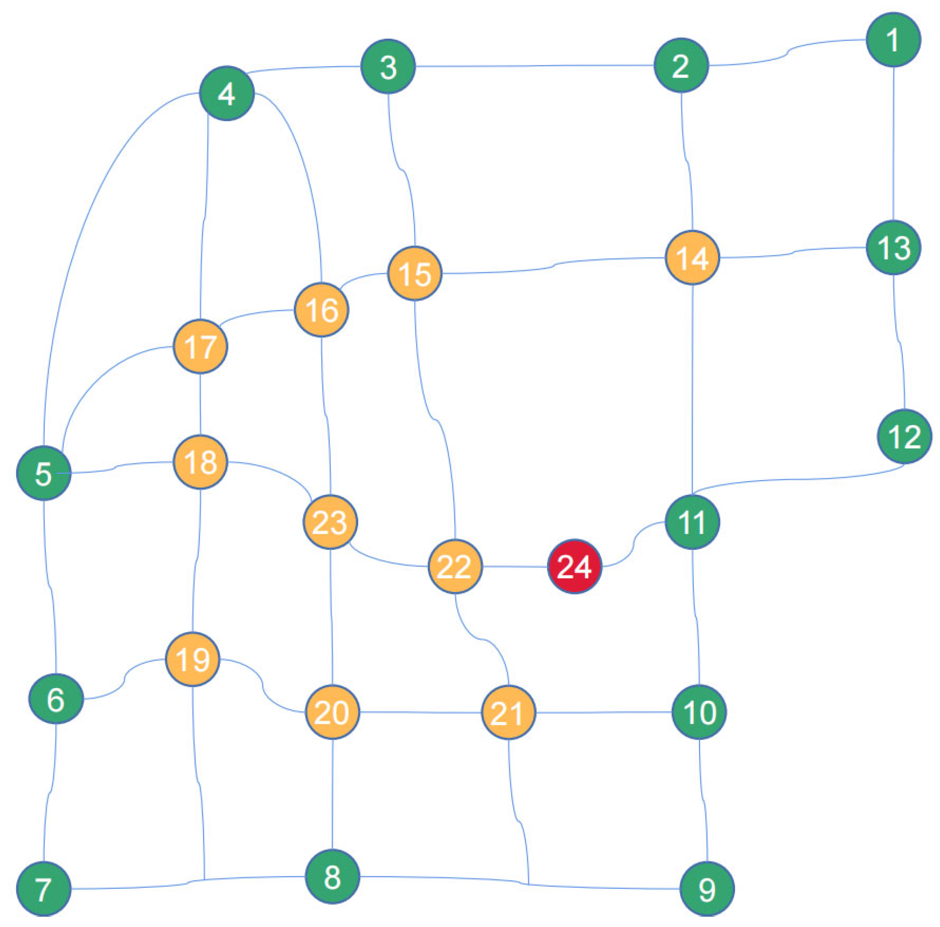
According to the location model of the BSS above, we choose 24 places in the region around Xizhimen, Beijing and combined them with the road information to build a virtual road network. The location of the 24 selected places is shown as red markers in Figure 2. This virtual road network contains 24 stations, 6 north–south streets and 5 east–west streets. The road connectivity between these stations and the number of each station is shown in Figure 3. Among the 24 stations, stations 1–13 belong to class “station”, stations 14–23 belong to class “node”, and station 24 belong to class “terminal”, as is shown in

Table 1. Station information.

Class: Station	Class: Node	Class: Terminal
1, 2, 3, 4, 5, 6, 7, 8, 9, 10, 11, 12, 13	14, 15, 16, 17, 18, 19, 20, 21, 22, 23	24

.

First, based on the road network in Figure 3, we use TransCAD and the GA-FW method proposed in Section 2.3 to carry out the traffic flow assignment result separately. Then, we calculate the traffic flow considering road type as the classification dimension, comparing the tendency between traditional algorithm and GA-FW.

Based on the actual road network, this paper considers two different road hierarchy: expressway and arterial road. And the arterial road is divided into two types: road with 8 two-way lanes and road with 6 two-way lanes, in order to better approximate the actual road network situation. The two types of arterial road have different capacities, which are set to analyze the difference between the traffic assignment methods, whether roads at same hierarchy tend to have a similar flow and density without considering their capacity. After traffic flow assignment, the distribution tendency of different algorithms will be evaluated in 2 dimensions: tendency between roads on different levels of the hierarchy and tendency between roads on the same hierarchy level with different capacity.

The road information is shown in

Table 2. Road information.

Road ID	Road Name	Road Hierarchy	Number of Two-Way Lanes
1	1-2-3-4	Expressway	8
2	13-14-15-16	Expressway	8
3	16-17-5	Arterial Road	6
4	12-11	Expressway	8
5	11-24-22-23-18-5	Arterial Road	8
6	10-21-20-19-6	Arterial Road	6
7	9-8-7	Arterial Road	8
8	4-5-6-7	Expressway	8
9	4-17-18-19	Arterial Road	6
10	4-16	Arterial Road	6
11	16-23-20-8	Expressway	8
12	3-15-22-21	Arterial Road	6
13	2-14-11	Arterial Road	8
14	12-11-10-9	Expressway	8
15	1-13-12	Arterial Road	8

. The free-flow speed of expressway is 70 km/h. The free-flow speed of arterial road is 50 km/h.

As for the bus line, we consider 20 bus lines entering the region from these 13 stations. Considering that the forward and reverse directions of buses may affect the location selection, the forward and reverse directions of bus lines are regarded as two different lines in this paper, so there are 40 lines in total. The specific stopping information of the lines is shown in

Table 3. Bus line information.

Line ID	Entry Station ID	Passing Nodes	Exit Station ID
101	1	14, 15, 16, 17	5
102	2	14, 15, 22, 21	9
103	3	15, 16, 23, 20	8
104	4	16, 18, 19	6
105	5	17, 18, 23, 22, 24	11
106	6	19, 20, 21	10
107	7	19, 18, 17, 16, 15	3
108	8	20, 23, 16	4
109	9	20, 19, 18, 17	5
110	10	21, 20, 23, 16, 15, 14	13
111	11	24, 22, 21	9
112	12	14, 15, 16, 23, 20	8
113	13	14, 15, 16, 17	5
114	4	16, 23, 20, 21	10
115	4	16, 23, 22, 24	11
116	3	15, 16, 17	5
117	5	18, 17, 16, 15, 14	2
118	6	19, 20, 23, 16	4
119	9	21, 22, 15	3
120	10	21, 20, 19, 18, 17	4

.

First, based on the road network in Figure 3 we use TransCAD to carry out the traffic flow assignment based on the four-stage method, calculating the traffic flow of each road obtained by the traditional algorithm, and then using the GA-FW algorithm proposed in Section 2.3 to obtain the difference between the two algorithms in traffic flow assignment.

Second, as a public infrastructure, the primary task of the BSS is to ensure the electric bus system is running orderly and efficiently. In order to meet the demand of electric buses to the greatest extent, the optimization goal is set under a maximum total battery capacity of the BSS. This paper considers the situation of maximum instantaneous charging demand, which means a 40-charging demand from 40 lines appearing at the same time. The 40-charging demand is distributed to the BSSs and achieves a minimum value of the objective function.

4. Result

In this paper, TransCAD and GA-FW are respectively used for traffic flow assignment. In TransCAD, a total of 28 traffic zones are divided and after travel production and travel distribution, the OD matrix is obtained. The global optimal algorithm method is used for TransCAD traffic assignment. In traditional GA, the population size is 50, maximum iterations time is 200, mutation probability is 0.05, crossing probability is 0.8. In this paper, the three hierarchies of roads are counted respectively and the traffic flow results of both directions is added to evaluate the intentions of different algorithms in terms of different road hierarchy. The result is shown in Figure 4.

The maximum flow of the expressway, 8-lane arterial road and 6-lane arterial road from TransCAD global optimal algorithm is 2709, 2388 and 1689, while it is 1567, 1843 and 1320 from GA-FW. Compared with TransCAD, an overall increase of −2.4% for expressway flow is achieved, while the rate is 4.4% and 10% for 8-lane arterial road and 6-lane arterial road.

Based on the global traffic flow obtained by the two methods, we analyze the optimal BSS location planning model for 40 bus lines. Due to old technology and aging batteries, the current mileage of bus vehicles used in some cities is only about 150 km. Road congestion, weather condition, and whether or not AC is turned on will also greatly affect the consumption of electricity. In extreme cases, the battery compacity can be reduced by more than 20% from the nominal range. So, the $e_{warning}$ is set to 0.15 and $e_{safe}$ is set to 0.05. There can only be one designated charging station in each direction of each bus line. In modified GA, the population size is 20, maximum iterations time is 1000, mutation probability is 0.05, crossing probability is 0.9. The model output is the global optimal BSS location for each bus line in each direction. The result is shown in Figure 3 and

Table 4. BSS Node Information.

Assignment Method	BSS Node ID	Capacity	Covering Line
TransCAD	16	24	101, −101, 103, −103, 104, −104, 107, −107, 108, −108, 110, −110, 112, −112, 113, −113, 114.−114 116, −116, 117, −117, 118, −118
	18	3	109, −109, −120
	21	7	102, −102, 106, −106, 119, −119, 120
	24	6	105, −105, 111, −111, 115, −115
GA-FW	16	24	101, −101, 103, −103, 104, −104, 107, −107, 108, −108, 110, −110, 112, −112, 113, −113, 114, −114 116, −116, 117, −117, 118, −118
	20	3	109, −109, −120
	21	7	102, −102, 106, −106, 119, −119, 120
	24	6	105, −105, 111, −111, 115, −115

¹ Negative value indicates the reverse direction of the corresponding line.

.

Including terminal 24, a total of four nodes are selected as BSSs for both TransCAD and GA-FW. Among them, node 16 has the largest expected capacity and has to be responsible for the battery swapping demand from a total of 24 lines from both directions. The number is 7 for node 21 and 6 for terminal 24.

The main differences are the BSS selected for line 109, line −109 and line −120. The result is node 18 under TransCAD flow while it is node 20 under GA−FW flow, as is shown in Figure 5. Except for bus line 120, the positive and negative directions of the other lines’ BSS are all at the same station. The BSS of line 120 is node 21 when it runs the positive direction, and node 20 for the reverse station.

Through the above comparative analysis, it can be determined that TransCAD traffic flow distribution will give more priority to the distribution of the expressway. This is because when TransCAD establishes the network and impedance matrix, it considers the differences in design speed and road capacity caused by different road properties, so it will give priority to the distribution of traffic flow to the road with higher road grade. In the process of path selection, the GA-FW algorithm considers the minimum global impedance from the perspective of system optimization, so it will not only consider the differences caused by different road hierarchy, but also the situation of the whole road network when allocating. So, the flow will be allocated to the lower-grade roads with higher accessibility to alleviate the pressure of some higher-grade road. Compared with TransCAD, the objective function value based on GA-FW is reduced by 1.7%. Node 18 is a crossing of two 6-lane arterial roads, while node 20 is an expressway and 6-lane arterial road according to the road information above. The path from node 20 to node 16 is a straight stretch of expressway and node 20 is directly connected with node 16. The accessibility between node 20 and the other selected nodes is higher than node 18. Under some emergency situation, node 20 can better reduce the battery swapping pressure from the other two BSSs.

5. Conclusions

As electric buses gradually replace traditional buses to become the mainstream power type, it is becoming more and more important to optimize the location of the BSS in advance while planning urban transportation. Actually, there are few researchers focused on electric buses, let alone the combination of traffic flow and the location strategy. We focus on the field of electric bus BSSs, proposed a traffic flow assignment algorithm, and made some innovative explorations by combining the road congestion with the location problem of bus BSSs.

In this paper, a traffic flow assignment algorithm based on GA-FW optimization method is proposed. Compared with the traditional traffic flow assignment method, the GA-FW method tends to allocate more flow to the lower-hierarchy roads and reduces the flow pressure of the higher-hierarchy roads. This method is proved to be closer to the global optimal. Based on the traffic flow results from the two algorithms, a BSS selection simulation of the bus changing station in the simulated road network is carried out. Under the guidance of GA-FW algorithm, the location plan for electric bus BSSs has achieved a lower total service cost with higher accessibility. The result is more conducive to the peak battery swapping demand.

For public transit operators, an appropriate location for BSSs can reduce the operational costs of buses, reduce energy expenditures, and optimize their management. For society and the environment, this can improve the environmental friendliness of buses and reduce greenhouse gas emissions. For public transportation policies, BSSs can simplify the charging process, increase bus route coverage, improve bus utilization, and thereby enhance the service quality.

However, due to the complexity of the electric bus system, there are still many issues this paper has not covered. First, this paper does not quantitatively describe the advantages of the GA-FW algorithm from the perspective of road congestion level. Secondly, this paper assumes that the capacity of a BSS can be unlimited, which is impossible in the real world. Follow-up work can take traffic congestion and the power grid’s acceptance into consideration, and both the total service cost and BSS maximum capacity are evaluated at the same time while planning a BSS’s location.