
Electric Vehicle Range Estimation Using Regression Techniques


Abstract
:1. Introduction
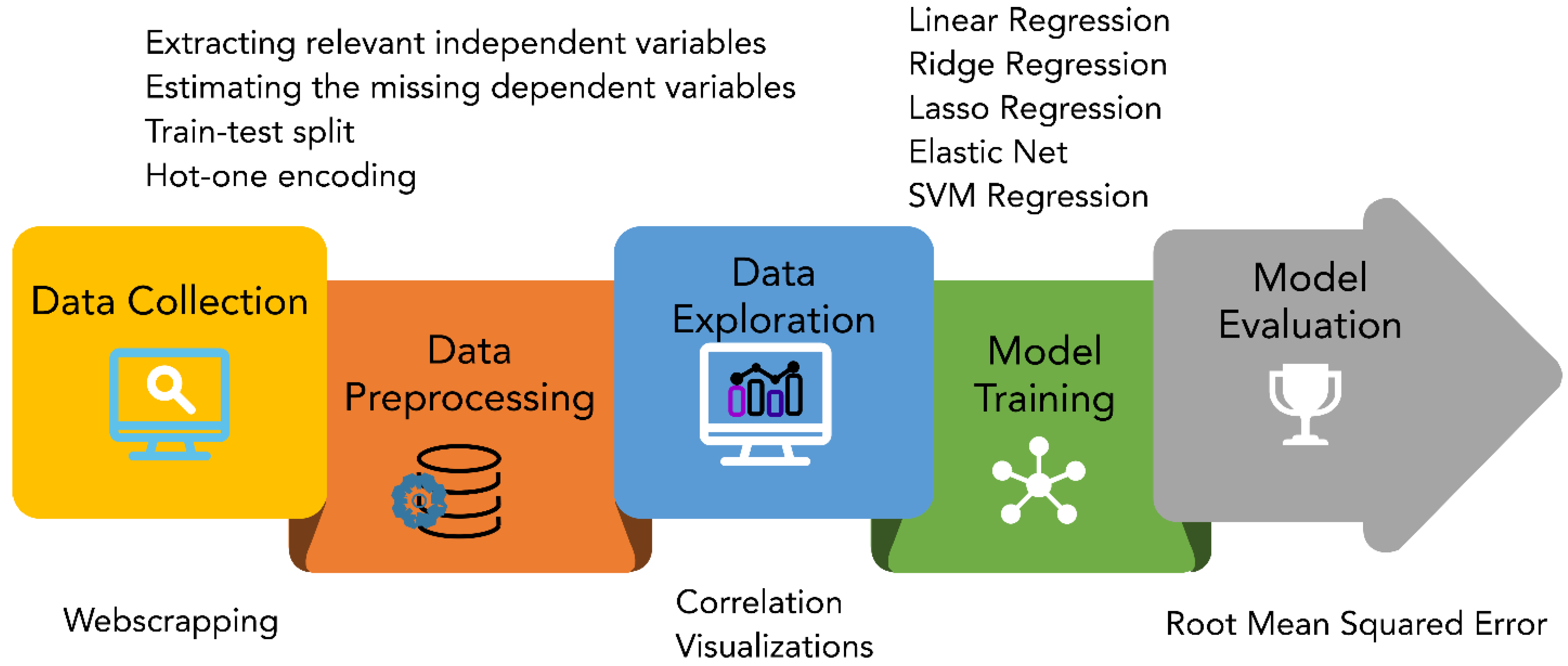
2. Methodology
2.1. Data Collection and Preprocessing
2.2. Regression Techniques
2.2.1. Linear Regression
2.2.2. Support Vector Machine
2.2.3. Model Training
2.2.4. Model Evaluation
3. Results and Discussion
4. Conclusions
Supplementary Materials
Author Contributions
Funding
Institutional Review Board Statement
Informed Consent Statement
Data Availability Statement
Conflicts of Interest
References
- Rietmann, N.; Hügler, B.; Lieven, T. Forecasting the Trajectory of Electric Vehicle Sales and the Consequences for Worldwide CO2 Emissions. J. Clean. Prod. 2020, 261, 121038. [Google Scholar] [CrossRef]
- Ellingsen, L.A.W.; Singh, B.; Strømman, A.H. The Size and Range Effect: Lifecycle Greenhouse Gas Emissions of Electric Vehicles. Environ. Res. Lett. 2016, 11, 054010. [Google Scholar] [CrossRef]
- Ma, H.; Balthasar, F.; Tait, N.; Riera-Palou, X.; Harrison, A. A New Comparison between the Life Cycle Greenhouse Gas Emissions of Battery Electric Vehicles and Internal Combustion Vehicles. Energy Policy 2012, 44, 160–173. [Google Scholar] [CrossRef]
- Perkins, J.H. Changing Energy: The Transition to a Sustainable Future; University of California Press: Oakland, CA, USA, 2017; ISBN 9780520287792. [Google Scholar]
- Wu, Z.; Wang, M.; Zheng, J.; Sun, X.; Zhao, M.; Wang, X. Life Cycle Greenhouse Gas Emission Reduction Potential of Battery Electric Vehicle. J. Clean. Prod. 2018, 190, 462–470. [Google Scholar] [CrossRef]
- Adnan, N.; Nordin, S.M.; Rahman, I.; Vasant, P.M.; Noor, A. A Comprehensive Review on Theoretical Framework-Based Electric Vehicle Consumer Adoption Research. Int. J. Energy Res. 2017, 41, 317–335. [Google Scholar] [CrossRef]
- Ahmed, M.; Zheng, Y.; Amine, A.; Fathiannasab, H.; Chen, Z. The Role of Artificial Intelligence in the Mass Adoption of Electric Vehicles. Joule 2021, 5, 2296–2322. [Google Scholar] [CrossRef]
- Good, D. EPA Test Procedures for Electric Vehicles and Plug-in Hybrids DRAFT Summary-Regulations Take Precedence. 2017. Available online: www.fueleconomy.gov (accessed on 14 March 2022).
- Mock, P.; Kühlwein, J.; Tietge, U.; Franco, V.; Bandivadekar, A.; German, J. The WLTP: How a New Test Procedure for Cars Will Affect Fuel Consumption Values in the EU. Int. Counc. Clean Transp. 2014, 9, 3547. [Google Scholar] [CrossRef]
- How Does The EPA Calculate Electric Car Range?|CleanTechnica. Available online: https://cleantechnica.com/2020/08/18/how-does-epa-calculate-electric-car-range/ (accessed on 11 September 2021).
- Mruzek, M.; Gajdáč, I.; Kučera, Ľ.; Barta, D. Analysis of Parameters Influencing Electric Vehicle Range. In Procedia Engineering; Elsevier Ltd.: Amsterdam, The Netherlands, 1 January 2016; Volume 134, pp. 165–174. [Google Scholar]
- Rastani, S.; Yüksel, T.; Çatay, B. Effects of Ambient Temperature on the Route Planning of Electric Freight Vehicles. Transp. Res. Part D Transp. Environ. 2019, 74, 124–141. [Google Scholar] [CrossRef]
- Hayes, J.G.; de Oliveira, R.P.R.; Vaughan, S.; Egan, M.G. Simplified Electric Vehicle Power Train Models and Range Estimation. In Proceedings of the 2011 IEEE Vehicle Power and Propulsion Conference, VPPC 2011, Chicago, IL, USA, 6–9 September 2011; IEEE: Piscataway, NJ, USA, 2011. [Google Scholar] [CrossRef]
- Bolovinou, A.; Bakas, I.; Amditis, A.; Mastrandrea, F.; Vinciotti, W. Online Prediction of an Electric Vehicle Remaining Range Based on Regression Analysis. In Proceedings of the 2014 IEEE International Electric Vehicle Conference, IEVC 2014, Florence, Italy, 17–19 December 2014; IEEE: Piscataway, NJ, USA, 2014. [Google Scholar] [CrossRef]
- Minett, C.F.; Salomons, A.M.; Daamen, W.; Van Arem, B.; Kuijpers, S. Eco-Routing: Comparing the Fuel Consumption of Different Routes between an Origin and Destination Using Field Test Speed Profiles and Synthetic Speed Profiles. In Proceedings of the 2011 IEEE Forum on Integrated and Sustainable Transportation Systems, FISTS 2011, Vienna, Austria, 29 June–1 July 2011; IEEE: Piscataway, NJ, USA, 2011; pp. 32–39. [Google Scholar] [CrossRef]
- Fiori, C.; Ahn, K.; Rakha, H.A. Power-Based Electric Vehicle Energy Consumption Model: Model Development and Validation. Appl. Energy 2016, 168, 257–268. [Google Scholar] [CrossRef]
- Shibata, S.; Nakagawa, T. Mathematical Model of Electric Vehicle Power Consumption for Traveling and Air-Conditioning. J. Energy Power Eng. 2015, 9, 269–275. [Google Scholar] [CrossRef] [Green Version]
- Abousleiman, R.; Rawashdeh, O. Energy Consumption Model of an Electric Vehicle. In Proceedings of the 2015 IEEE Transportation Electrification Conference and Expo, ITEC 2015, Dearborn, MI, USA, 14–17 June 2015; IEEE: Piscataway, NJ, USA, 2015. [Google Scholar] [CrossRef]
- Barcellona, S.; de Simone, D.; Grillo, S. Real-Time Electric Vehicle Range Estimation Based on a Lithium-Ion Battery Model. In Proceedings of the ICCEP 2019—7th International Conference on Clean Electrical Power: Renewable Energy Resources Impact, Otranto, Italy, 2–4 July 2019; IEEE: Piscataway, NJ, USA, 2019; pp. 351–357. [Google Scholar] [CrossRef]
- Miri, I.; Fotouhi, A.; Ewin, N. Electric Vehicle Energy Consumption Modelling and Estimation—A Case Study. Int. J. Energy Res. 2021, 45, 501–520. [Google Scholar] [CrossRef]
- Kim, S.; Lee, J.; Lee, C. Does Driving Range of Electric Vehicles Influence Electric Vehicle Adoption? Sustainability 2017, 9, 1783. [Google Scholar] [CrossRef] [Green Version]
- EVSpecifications-Electric Vehicle Specifications, Electric Car News, EV Comparisons. Available online: https://www.evspecifications.com/ (accessed on 11 September 2021).
- Used 2018 Volkswagen E-Golf Specs & Features|Edmunds. Available online: https://www.edmunds.com/volkswagen/e-golf/2018/features-specs/ (accessed on 11 September 2021).
- Rodgers, J.L.; Nicewander, W.A. Thirteen Ways to Look at the Correlation Coefficient. Am. Stat. 1988, 42, 59. [Google Scholar] [CrossRef]
- Geron, A. Regularized Linear Models. In Hands-On Machine Learning with Scikit-Learn and TensorFlow; O Reilly: Springfield, MO, USA, 2019; pp. 134–141. [Google Scholar]
- Geron, A. Support Vector Machines. In Hands-On Machine Learning with Scikit-Learn and TensorFlow; O Reilly: Springfield, MO, USA, 2019; pp. 153–174. [Google Scholar]
- Geron, A. Linear Regression. In Hands-On Machine Learning with Scikit-Learn and TensorFlow; O Reilly: Springfield, MO, USA, 2019; pp. 112–117. [Google Scholar]
- Gao, C.; Bompard, E.; Napoli, R.; Cheng, H. Price Forecast in the Competitive Electricity Market by Support Vector Machine. Phys. A Stat. Mech. Its Appl. 2007, 382, 98–113. [Google Scholar] [CrossRef]
- Gu, J.; Zhu, M.; Jiang, L. Housing Price Forecasting Based on Genetic Algorithm and Support Vector Machine. Expert Syst. Appl. 2011, 38, 3383–3386. [Google Scholar] [CrossRef]
- Scikit-Learn: Machine Learning in Python—Scikit-Learn 0.24.2 Documentation. Available online: https://scikit-learn.org/stable/ (accessed on 8 June 2021).
- Vapnik, V. SVM for Estimating Regression Function. In The Nature of Statistical Learning Theory; Springer: Berlin, Germany, 1995; pp. 183–188. [Google Scholar]
- Ma, Y.; Zhang, Z.; Ihler, A.; Pan, B. Estimating Warehouse Rental Price Using Machine Learning Techniques. Int. J. Comput. Commun. Control 2018, 13, 235–250. [Google Scholar] [CrossRef] [Green Version]
- Plett, G. Simulating Battery Packs. In Battery Management Systems, Volume 2; Artech House: Norwood, MA, USA, 2015; pp. 31–67. [Google Scholar]
- CER—Market Snapshot: Average Electric Vehicle Range Almost Doubled in the Last Six Years. Available online: https://www.cer-rec.gc.ca/en/data-analysis/energy-markets/market-snapshots/2019/market-snapshot-average-electric-vehicle-range-almost-doubled-in-last-six-years.html (accessed on 3 June 2021).
- Yakkundi, V.; Mantha, S.; Sunnapwar, V. Hatchback versus Sedan—A Review of Drag Issues. Int. J. Mech. Eng. 2017, 4, 5–13. [Google Scholar] [CrossRef] [Green Version]
- Lu, M.; Zhang, X.; Ji, J.; Xu, X.; Zhang, Y. Research Progress on Power Battery Cooling Technology for Electric Vehicles. J. Energy Storage 2020, 27, 101155. [Google Scholar] [CrossRef]
- Chicco, D.; Warrens, M.J.; Jurman, G. The Coefficient of Determination R-Squared Is More Informative than SMAPE, MAE, MAPE, MSE and RMSE in Regression Analysis Evaluation. PeerJ Comput. Sci. 2021, 7, e623. [Google Scholar] [CrossRef] [PubMed]
- Saunders, L.; Russell, R.; Crabb, D. The Coefficient of Determination: What Determines a Useful R2 Statistic? Investig. Ophthalmol. Vis. Sci. 2012, 53, 6830–6832. [Google Scholar] [CrossRef] [PubMed] [Green Version]


| Variables | Correlations |
|---|---|
| Battery Capacity (kWh) | 0.903860 |
| Top Speed (mph) | 0.794916 |
| Curb Weight (lb) | 0.700247 |
| Number of Battery Cells | 0.689241 |
| GVWR (lb) | 0.660293 |
| Model Year | 0.262226 |
| Voltage (V) | 0.187742 |
| Number of Battery Modules | 0.041696 |
| Acceleration from 0 to 100 km/h (s) | −0.839825 |
| Model | Parameters |
|---|---|
| Normal Linear Regression | - |
| Ridge Regression | α = 1 |
| Lasso Regression | α = 0.1 |
| Elastic Net | α = 0.1 |
| r = 0.5 | |
| SVM Regression | ε = 0.1 |
| C = 1 |
| Model | RMSE |
|---|---|
| Normal Linear Regression | 33.200 |
| Ridge Regression | 33.540 |
| Lasso Regression | 33.084 |
| Elastic Net | 37.423 |
| SVM Regression | 31.428 |
Publisher’s Note: MDPI stays neutral with regard to jurisdictional claims in published maps and institutional affiliations. |
© 2022 by the authors. Licensee MDPI, Basel, Switzerland. This article is an open access article distributed under the terms and conditions of the Creative Commons Attribution (CC BY) license (https://creativecommons.org/licenses/by/4.0/).
Share and Cite
Ahmed, M.; Mao, Z.; Zheng, Y.; Chen, T.; Chen, Z. Electric Vehicle Range Estimation Using Regression Techniques. World Electr. Veh. J. 2022, 13, 105. https://doi.org/10.3390/wevj13060105
Ahmed M, Mao Z, Zheng Y, Chen T, Chen Z. Electric Vehicle Range Estimation Using Regression Techniques. World Electric Vehicle Journal. 2022; 13(6):105. https://doi.org/10.3390/wevj13060105
Chicago/Turabian StyleAhmed, Moin, Zhiyu Mao, Yun Zheng, Tao Chen, and Zhongwei Chen. 2022. "Electric Vehicle Range Estimation Using Regression Techniques" World Electric Vehicle Journal 13, no. 6: 105. https://doi.org/10.3390/wevj13060105