1. Introduction
The number of electric vehicles (EVs) is expected to increase exponentially in the coming years [
1,
2]. To meet this rise in EV growth, policy makers and market parties are increasingly deploying several private, semi-public, and public charging points, both AC and DC. The growing presence of charging points generates a multitude of interactions between EV users, particularly in metropolitan areas, where a charging infrastructure is largely part of the public domain [
3].
The planning of public AC charging infrastructure (CI) is challenging, as (i) multiple stakeholders with different interests are involved; (ii) the required public space for CI is scarce and needs to be weighed with other public interests [
4,
5], and (iii) CI needs to facilitate charging needs of different modalities [
6,
7,
8]. Yet, policy makers are limited in their choices as to when and where to deploy what type of CI. For policy makers, developing public CI is a balancing act to reduce over-dimensioning (leading to high investments and public scrutiny), as well as under-dimensioning of available CI (leading to limited access of EV users) [
9,
10].
Since the first release of modern EVs, researchers and policy makers have shown an interest in zero emission mobility [
11], particularly in the planning of public charging infrastructure and how policy makers may optimize its development and deployment [
12]. Researchers have traditionally analyzed and optimized charging infrastructure through a demand-side approach to charging infrastructure planning. This approach encompasses an estimated charging demand (i.e., the number of charging points or kWh) as input for planning methods [
13]. Planning methods involve (i) planning using spatial operational research methods [
14,
15], (ii) data-driven methods using spatiotemporal presence of vehicles (mostly non-EV) data [
16,
17], and (iii) models focused on charging behavior [
18]. The problem with these models is that they are unable to fully capture the complexity of charging behavior and EV user interactions [
1]. The use of these models induces a linear scaling between the system’s supply (CPs) and demand (EVs). As a result, predictions from linear models may lead to overestimation of charging infrastructure performance and underestimation of its convenience for EV users [
1]. Inaccurate predictions can result in the under- and oversupply of CPs, leading to ineffective deployment strategies and inefficient use of CI. It is, therefore, important for both researchers and policy makers to carefully choose an appropriate scientific approach that includes the dynamics of the EV system (CPs, EVs, policy makers, and supporting charging infrastructure), in order to effectively deploy and use this system. This understanding is also important for policy makers, as interventions in the EV system to optimize efficiency may have unexpected, counterproductive outcomes. We see that, despite the sheer volume of literature, little attention has been paid to the characteristics, variance, and interdependencies of the behavior in EV systems.
This research contributes to current literature by proposing guidelines for selecting a scientific approach, given the properties of charging infrastructure (e.g., charger type or network density). We do so by providing an abstraction of charging infrastructure, as a system of supply and demand, in which social interactions take place. Systems in which social behavior plays a role may contain tipping points and regime changes, in which the dynamics that generate the data fundamentally change when the system changes [
19,
20,
21,
22]. We call these systems complex, in which the complexity lies in the limited ability of models to predict the system’s future states using the knowledge of its current state [
19,
20,
22]. Our proposed guidelines include three ratios that estimate the rate of complexity in the system. We suggest how typical aspects of complex systems can be applied to public charging infrastructure, in order to offer a deeper scientific understanding of the dynamics of EV charging. We expect that the use of complex systems methods analysis helps to improve the accuracy of simulation studies.
In this research, we use a two-step approach. In
Section 2, we introduce the concept of social supply–demand systems (SSDSs) as a specific version of a publicly available resource (or common-pool resource (CPR)) [
21], such as public charging points. We provide a mathematical notation of its main constituting elements. We argue that properties of SSDS systems may be understood by taking a complex systems perspective. In
Section 3, we describe the most prominent complex system properties and reflect on its suitability to describe charging infrastructure utilization. In
Section 4, we develop metrics to estimate and compare the complexity in SSDS systems and reflect on complexity of different CI systems. Based on the values of these metrics, we propose how to use a complex systems methodology to analyze and model the utilization of charging infrastructure (
Section 5). Finally, in
Section 6, we elaborate on the consequences, for both research and policy makers, when the complex systems approach is applied.
2. General Abstraction of Infrastructures as Systems of Supply and Demand
In economic theory, the consumption of publicly accessible goods from a large pool, which may exclude users from consuming resources and where one user’s large consumption may preclude other users, is called a common-pool resource (CPR) problem [
21]. Examples of such systems are open natural systems (fishery, land use) [
21,
23]. The lack of a central controller in such systems leads to behavioral questions of resource allocation, free riding, and collaboration [
24]. A central theme of CPR is the sustainable use of the resources to avoid depletion [
21,
25,
26]. Researchers have argued that public infrastructures may conceptually be seen as a non-excludable and -exhaustive resource and, hence, as a CPR [
27], although mathematical derivations have pointed to significant differences due to rivalry [
23].
A particular variant of a CPR is a so-called social supply–demand system (SSDS). An SSDS is a system with two kinds of entities (supply and demand), in which resources from an infinite pool are transferred at a limited set of outlets from an individual item of one kind (the supply side) to an individual item of the other kind (the demand side). The social part of SSDS relates to interactions between elements (either of the same kind or between both kinds), which results in non-trivial behavioral patterns. The term non-trivial, in our definition, means behavior that changes non-linearly when scaling the system’s size by increasing the number of entities. The key differences between CPR and SSDS are as follows. In an SSDS, transactions of the supply side are subject of research, rather than the consumption (in size) of the common-pool resource. In an SSDS, the complex interactions occur due to the small size of the supply side outlets, compared to the size of the population, whereas in CPR the resource pool is small, compared to the demand. In an SSDS, the focus is on the growth (deployment) or decline of the system, in terms of the size of supply and demand side elements, rather than depletion of the resource pool. As such, SSDS provide opportunities for studying CI, as CI is also characterized as a supply–demand, with a limited set of outputs and social component.
The challenges of understanding SSDS dynamics have been explored for other systems (
Table 1). Some systems have a strong technological component (e.g., electricity and traffic), while others have a larger social behavior component or are based on natural systems. The dynamics that are researched using complex systems theory vary from analysis of emergent phenomena (segregation of education) to path dependency (healthcare) and resilience to perturbations (energy grids). In the following, learnings from these cases are used to generate key variables in characterizing SSDS, which can be translated in mathematical notations.
SSDS have spatially fixed resource access points, each with a specific number of outlets that constantly offer the resources at outlets at a particular rate. The users of this system require this resource and occupy the outlets of the access points for finite time periods, in which they load a finite volume of the resource, sometimes with a specific quality. Once all outlets at an access point are occupied, the access point is said to be occupied. The users’ desire or ability to wait or choose another access point, or their willingness to cooperate with other users to share outlets at resources access points, is user- and context-dependent.
The system contains several types of entities: the environment (), resources access points (), and users (). Next, the system contains transactions () between resources and users. More formally, the system is characterized by an environment () that can be of any size (e.g., an x–y plane), spatially distributed resource access points , each with a finite number of outlets, set of spatially mobile users , and set of transactions made by users. A transaction is a mapping between one element of and U at a specific time (). Any user () can have multiple transactions on any number of freely selected elements (), but these transactions cannot be simultaneous.
We define an SSDS as having the following conditions: condition (i)
, which means that there are typically more users than resources, and condition (ii)
which means that there are typically more transactions than users. Condition (i) allows for scarcity and competition in the system. Condition (ii) needs to be satisfied to allow the system to process learning effects and habits in user behavior. For the EV system, there are typically more EV users than public CPs and many more transactions than users (e.g., 4.3 M transactions for 29 k users at 5000 resources access points [
3]).
A characteristic of SSDS is the change in size (both growth and decline) of both the user base (U) and number of resource access points () over time. As a result, the set of transactions () may display an increased pace of growth (second partial derivative) over time (e.g., traffic density increases or increased pressure on health facilities during a pandemic). Resources may be added, removed, or moved to balance of local supply and demand of resources. The local optimal ratio to vary over space and time and are dependent on the distribution of the service rate and scaling effects as part of supply side network density.
2.1. Environment
The environment in many SSDSs is a finite space in a two-dimensional coordinate system, such that
(
Table 1). Alternatively, the environment can be modelled as a network grid (e.g., electricity network). A location (
) is defined as a point in space, such that
.
The properties of each location (
) may be bound by several constraints. First, a maximum number of resource outlets for each location may apply, as well as a maximum number of users per location. Additionally, some systems may contain a set of constraints on the maximum supply rate in specific areas of the environment (e.g., electricity grids). Other systems, however, may be constrained by the local production of resources at locations (e.g., natural systems). The EV system is often modelled as a 2D space, bounded by physical constraints [
34].
In many SSDSs, the distribution of the resource access points in the environment is expected to influence the behavior within the system [
28,
35]. For instance, resource access points may be distributed in a physically connected manner, in such a way that the flow rate at one outlet may be affected by other outlets (e.g., energy grids and transport of healthcare assets between hospitals). In such a network of connected elements, an outage of one outlet may lead to a sudden supply–demand at other outlets in the network [
33,
36]. Alternatively, resource access points may also form a network of alternative resource outlets, when the distance between resources outlets is such that they are considered by users. A typical example is found in the school choice, where the location distribution of schools affects selection [
28].
Finally, some systems have requirements set on the coverage of the environment. Healthcare or school facilities, for instance, are distributed such that, for any location (
) in the system, a resource outlet is located within a distance smaller than a threshold set by the government. For the EV system, policy makers are striving for an optimal coverage of the charging network, while balancing the needs of different stakeholders (e.g., grid providers and (non-)EV users) [
9].
2.2. Resource Access Points
Each resource access point (
) is characterized by a collection of properties, defined as a tuple:
. Each
is located at a unique
, with coordinates according to the dimensions of the environment (E). It has a set of outlets
=
that allow concurrent connection (e.g., number of beds in a hospital and number of sockets per charging point). Each
has a maximum throughput rate, which is the service rate (
). In some cases, the service rate is averaged or a standard over all outlets (e.g., electricity system). In other cases, each outlet may have a specific service rate, depending on the transaction that takes place at the outlets (surgery vs. long intensive care use within a hospital). The quality (
) of the resources supplied during transaction may play a role in some systems (e.g., education) and may also correlate to additional properties (e.g., pricing). At any given time (
) an outlet at
can be in status
, in which 0 is non-occupied idle and 1 is occupied transferring resources. Some specific systems allow for an extra status for being occupied without transfer of resources, which enables the efficiency optimization of resource utilization [
37].
In the simplest abstraction of this kind of system, resource access points do not communicate with each other, and users are not centrally steered towards the resource access points. In short, the resources are passive outlets that respond to user demand. This implies that the resource access points do not share information on the system’s status or actively transfer resources between each other, but only to the user. Users cannot gain information on the system’s state through the resource outlets. As such, the system configuration (supply side and demand side layout) is an important factor that determines the complexity of behavior in the system.
2.3. Users
Users in the system are individual entities making decisions for resource uptake at resource access points, based on individual optimization rewards. A user’s collection of decisions (set of transactions) is regarded as the user’s behavior. This base behavior may show rational or habitual behavioral patterns. The rational part of behavior involves decisions for choosing specific outlets for their resources, based on cost and benefit factors [
38]. These factors can be related to resource access points (
) (transaction supply speed), user specific properties (user specific preferences), or contextual properties (e.g., distance of a user to resource access points at that moment of deciding). The habitual part of each user’s behavior is found in the selection from a preferred or specific set of resource access points for a given location, arrival time, or place [
3,
15].
More formally, in the simplest abstraction, users are characterized by a given set of properties and developing set of attributes, collected over time, defined as a tuple:
. Each user (
) has an internal storage (
) for storing resources, storage capacity (
) that describes the maximum speed of resource uptake of the user, and demand, in terms of frequency (
), quantity (
), and quality (
). The internal storage (
) and storage capacity (
) can affect the frequency of transaction (
) and transaction size (see
Section 2.4), implying that large storage leads to lower frequency of use and higher transaction volume. The set
contains the user’s transactions, from which behavioral rules may be derived.
In many systems, users may adapt behavior if the environment does not meet their expectations or they discover that different behavior is more rewarding. For example, if the outlets of the resource access points are unavailable, the user can decide to go to a different location than originally planned. If this location has an occupancy profile that better suits the user’s demand profile, a user may change its habits, preferring this location to that of the old one.
Users are present in the vicinity of other users or occupy resource outlets that other users were about to decide to use. This inevitably creates user interactions in the system. In the simplest abstraction of the system, users do not share information with, or adapt their behavior to, other users. In several systems, there is only limited information centrally available on resource selection (e.g., school or healthcare selection or route navigation). There are systems (e.g., ant or bee colonies) where information on distribution of resources is shared amongst the population [
12]. In these more complex abstractions of this system, users may share information or collaborate. These social interactions may generate more efficient use of the system; for example, a user that occupies an outlet could make place for another user [
39].
2.4. Transactions
A transaction is the successful result of a user instigated attempt to connect to a resource outlet at a resource access point. This mapping between an element of U () and outlet () at R () is stored as a tuple . This tuple () contains the start time () of the transaction, the is the connection duration, and is the size of the transaction. The size of the transaction may be described by a simple linear function (e.g., electricity current function) or can be more complex and even unquantifiable (e.g., health and education). Since a user may have multiple transactions at the same outlet, we specify such as the set of transactions of at .
When a user instigates a transaction, it observes part of the local resources in the system but has no complete information on the system state. The locality of available information produces a restricted preference set for users. This set is much smaller than the actual system size. In most systems, information on the used capacity of resource outlets is unknown for users.
It can be the case that, due to occupancy, a user needs to make multiple attempts to successfully connect to a resource location. Some systems (e.g., healthcare and education) have waiting lists (queues), where the actual demand for resources is stored. In other systems, successive attempts may lead to competition for resources (e.g., natural systems) or sudden stagnation of transfer (e.g., traffic jams). Finally, in some systems, the time of transferring resources is shorter than the actual connection time. This results in the resource outlet being connected in an idle state of the resource outlet, as mentioned earlier.
2.5. Research Methodologies for Charging Infrastructure as Social Supply–Demand System
In the previous sections, we showed a general abstraction of an SSDS. We concluded that charging infrastructure fits with the provided abstraction of SSDS. We also found existing systems that had a similar fit. A closer examination of research methodologies, used for similar systems, shows that complex systems have been used to model and understand the behavior in those systems (see references in
Table 1). This reinforces our original hypothesis that, when modeling the EV system, the complexity of behavior should be considered.
3. Charging Infrastructure as a Complex System
Complex systems (CS) are an approach towards system analysis that focuses on emerging structures at a macro level that are derived from micro-level behavior [
33]. The methods used in the CS have proven to provide a deeper understanding of systems that are difficult to predict from an individual level [
33]. The application of CS can be found in ecology, biology, healthcare, and social studies [
22,
40,
41,
42]. Additionally, CS has proven to support creating public policy making [
43] and analyzing critical infrastructures [
44].
Although an extensive amount of literature has been written on CS, there is neither a sharp definition nor a set of preconditions for a system to be complex [
22]. The concepts of complexity are embraced by other fields of science, each with its own emphasis on specific properties of complexity [
22]. Using properties, as described by Ladyman [
22], we define a CS as a system in which the number of interactions scales non-linearly with the number of interacting components, in which the initial conditions and perturbations strongly affect the behavioral regime and multiple pathways exist, to which the system can grow for the same given initial conditions [
22]. From this definition, a set of features was extracted. In the next sections, we propose how these features can be included in the analysis of the EV as a complex system.
3.1. Feedback Loops
Feedback loops are core elements of a CS that occur because interactions of elements in the system are inputs for future behavior of other elements [
22,
43]. The effect of the feedback loop on the behavior may be reinforcing (amplifying earlier behavior) or balancing (damping earlier behavior) [
45]. Effect loops vary in size (linear and non-linear [
45]), time scale (varying from instant to delayed [
43]), and aggregation scale (from individual level to the whole system [
46]). Examples of feedback loops can be found in natural systems of supply and demand (
Table 1), where prey (supply side) are eaten by predators (demand side). For instance, successful foraging strategies of predators lead to reinforced hunting strategies of individuals and groups (herds) [
46].
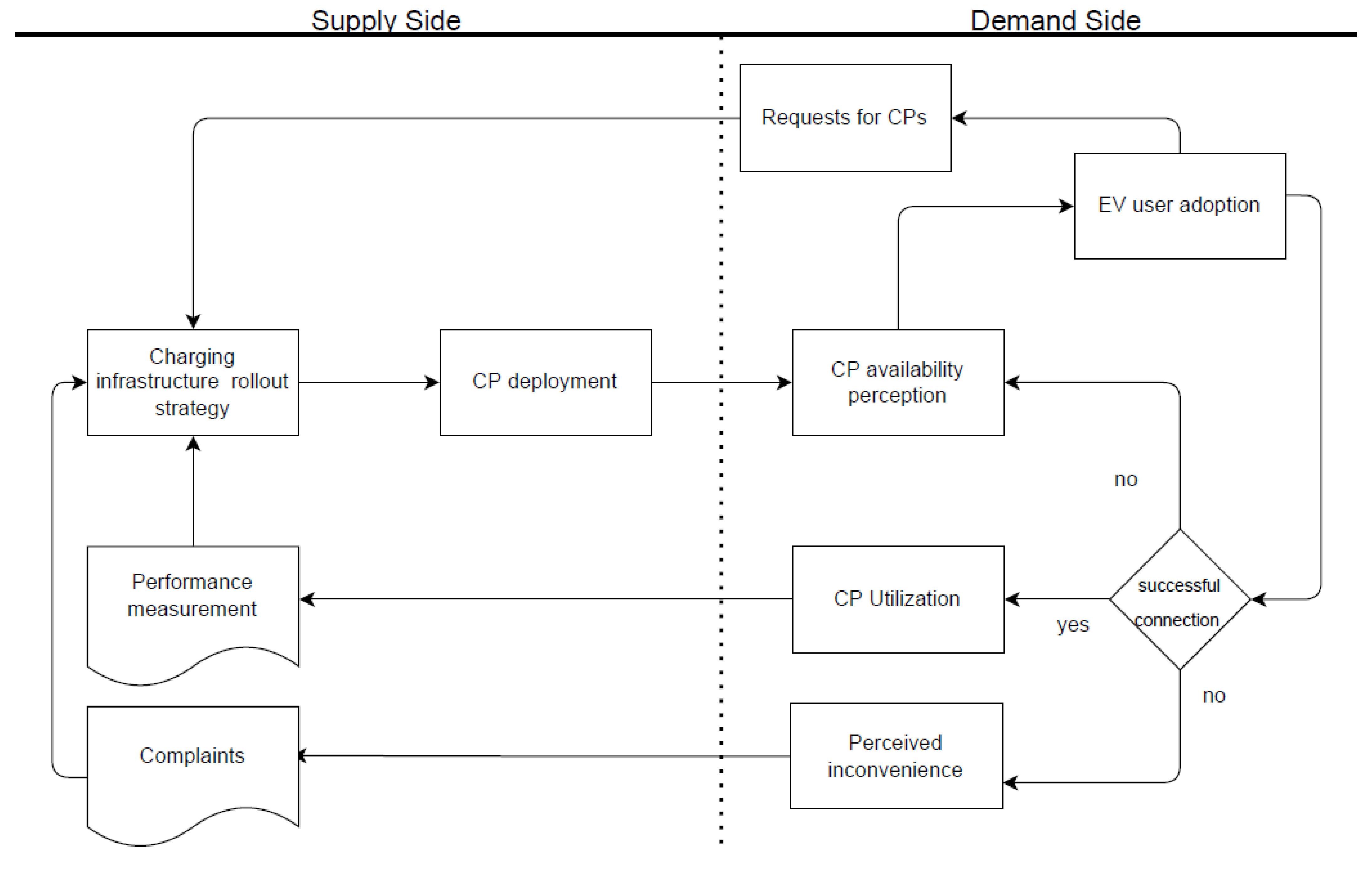
In the EV system, we see feedback loops, related to policy makers’ charging point deployment strategies (see
Figure 1) [
47]. Policy makers’ decisions on where and when to deploy CPs may include actual requests for CPs by EV owners, complaints from both EV and non-EV users, and key performance metrics (KPIs), based on charging data [
9,
48]. Policy makers may use CP performance metrics from charging data to evaluate decisions for CP locations [
48,
49]. This creates a feedback loop that may reinforce deployment decisions, even though policy makers may not have the full information on the system state [
50]. We also observe a feedback loop within the system, related to the demand side population growth, as the existence of CPs in an area has found attract new EV users [
1]. An increase of EV users will result in an increase of interactions and, hence, affect the other feedback loops. On the other hand, negative experiences with EV charging may result in EV users selling or not replacing their EV [
51].
3.2. Learning and Adaptation
Elements in a CS make autonomous decisions, in line with their set of behavioral rules and experiences. EV users may learn by adjusting their behavioral rules, based on experiences. We call this learning. Adaptation refers to elements of the system that can autonomously adapt their behavior to a changing environment [
22]. Changes may be sudden (perturbations) and present at the element level (e.g., addition of new demand side elements) or at the macroscale (climate changes).
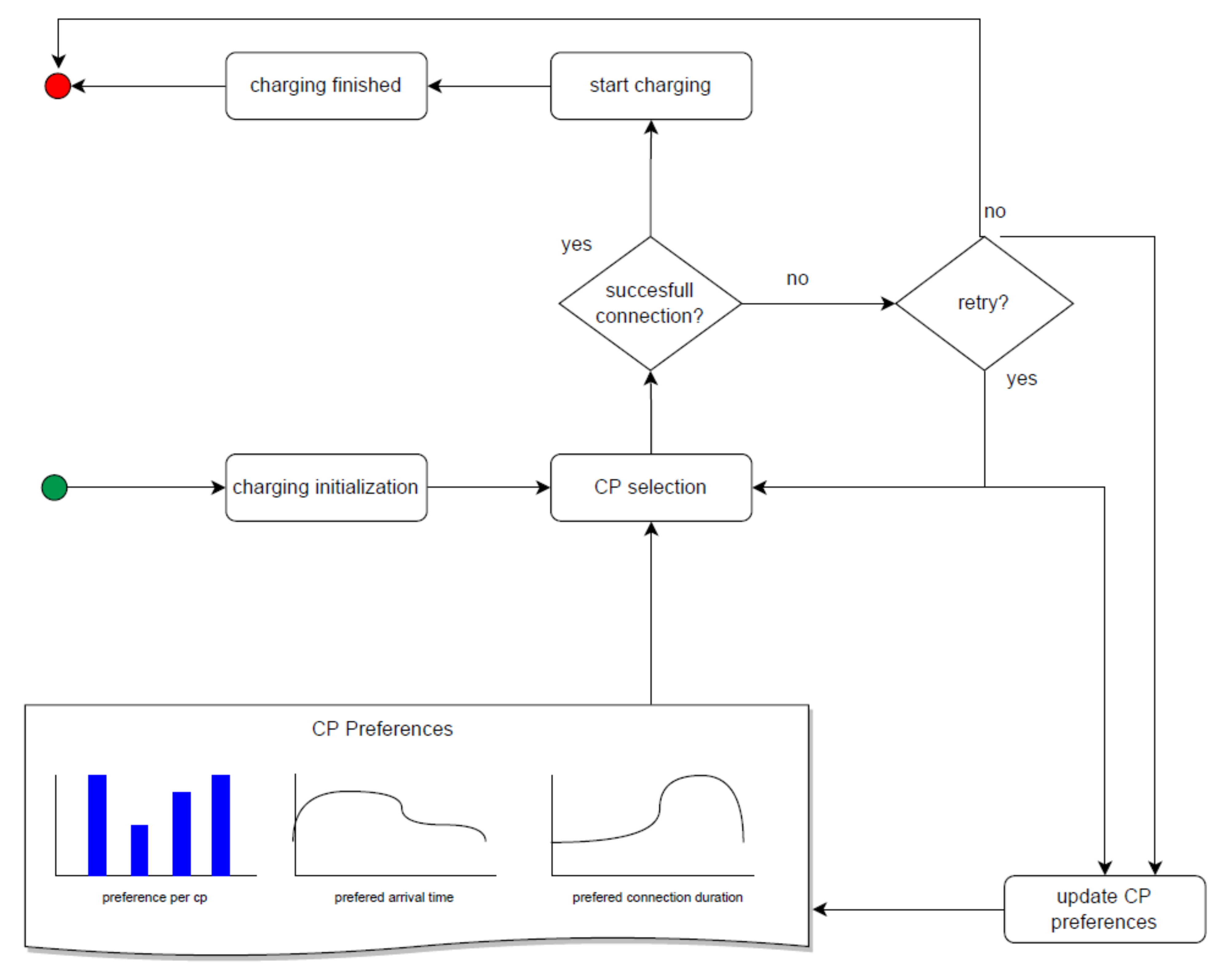
Within the EV system, learning is based on EV user experience and interactions during their use of charging infrastructure [
3]. At a user level, (un)successful charging behavior, in terms of CP selection in time and space, may lead to self-reinforcing behavior (illustrated in
Figure 2). It is assumed that EV users strive for the best convenience of charging and adapt their behavior to achieve this. Negative experiences, due to occupancy of preferred CPs, may, thus, shift behavior in when and where to charge. As an example, an EV user may decide to arrive earlier at a CP to increase the probability of occupying that CP or reroute to different CPs that have a lower occupancy rate, in order to be ensured a charging place [
3].
Similar to adaptation patters in natural systems, we expect that, due to increasing deployment of charging infrastructure, EV users will adapt their preferences to alternative CPs for reasons of distance or experienced occupancy (see
Figure 2) [
52,
53,
54]. Additionally, it has been found that pricing incentives also lead to adaptive charging behavior, in terms or arrival and departure times [
55].
At the macro scale, we expect adaptation of EV users, due to exogenous factors. As EV adoption matures (going from early adopters to mainstream EV users), we expect that charging demands will also change. Specific user types, such as taxis and car sharing, have adopted electric drivetrains lately [
56,
57]. User expectations and charging behavior of these groups is expected to differ. Existing EV users will adopt to the patterns of charging behavior of these new user groups, as they interact within the EV system.
3.3. Emergence
The literature has shown that interactions between elements may lead to unexpected spontaneous patterns of behavior at macro level, such as collaboration and competition [
58,
59]. These macro level patterns are known as emergent behavior. This type of behavior is neither part of the resource access point selection behavior nor controlled as a goal that the individuals strive for.
We see emergent patterns in many systems. A classic example is a flock of birds. All the birds want to be part of the flock, but the flock has no leader or centralized coordination [
60]. Additionally, traffic jams are emergent patterns that follow specific patterns, unrelated to individual driver behavior [
61,
62]. Research in critical infrastructures has revealed a tendency of these systems to react similarly to perturbations; the size of the reaction fits a power law [
62,
63]. The emergent pattern of reaction is neither centrally coordinated nor part of the individual elements.
As the EV system matures, and the density of an EV system increases, emergent patterns of competition between EV users for CPs or emergent patterns of scheduling may appear. Patterns of competition were found in earlier research that analyzes unsuccessful connection attempts of an EV user to a CP [
1]. The EV system may also exhibit a tendency to react to perturbations similar to critical infrastructures, as it is connected to other systems (i.e., electricity and road infrastructure). These emergent patterns are bound to affect the perceived convenience of using the EV system and create a feedback loop.
Regarding emergent patterns of scheduling, we expect a development towards subnetworks, similar with activity patterns within the charging network, will develop. A subset of CPs, that are all relevant alternatives to each other and share the same pool of EV users, will reveal similar patterns of arrival and departure. This, in turn, may lead to parts of the network being driven by competition or collaboration. In other subnetworks, we expect activity patterns to be driven by a local mixture of user types.
3.4. Network Formation and Resilience
Research has revealed that critical infrastructures tend to grow towards a network of connected elements, either physically connected or connected by overlapping behavioral choices [
33,
63]. This network structure may contain one or more large, connected components. The network is said to be robust when the network is able to accommodate perturbations in the system [
64,
65]. For example, when a perturbation in the system does not lead to a breakdown of the network or the perturbation of travels through a limited number of elements in the system [
66,
67,
68,
69,
70,
71,
72,
73,
74,
75,
76,
77,
78,
79,
80,
81,
82,
83,
84,
85,
86]. In this case, behavioral patterns tend to reoccur after recovery [
33]. On the other hand, a network is said to be vulnerable when perturbations pass through large parts of nodes in the network or the system is damaged and can no longer function [
65].
Research on vulnerability of complex networks has shown that, as the load in the system increases, cascading failures are more likely to occur [
7]. The likelihood of cascades does not gradually increase with system load, yet it reaches a critical point, at which the propagation of failures suddenly increases [
69,
70]. Therefore, during the design and operation of a system, the EV system load needs to be balanced with the system’s economic benefits. A fully loaded system may potentially lead to larger system failures, while suboptimal operation, in terms of load on the system, leads to a more robust system [
68]. Likewise, intelligent rerouting of load in a complex network may decrease the effect of perturbations but require some form of central steering in the system.
As the density of charging infrastructure increases, the number of relevant alternatives CPs within walking distance to a destination of an EV user increases, as well, which leads to a network of alternative charging points [
18]. Having more than one relevant alternative may lead to economies of scale and a lower required ratio of CPs per EV user. A negative effect of a denser charging network, however, may be the increased length of perturbations.
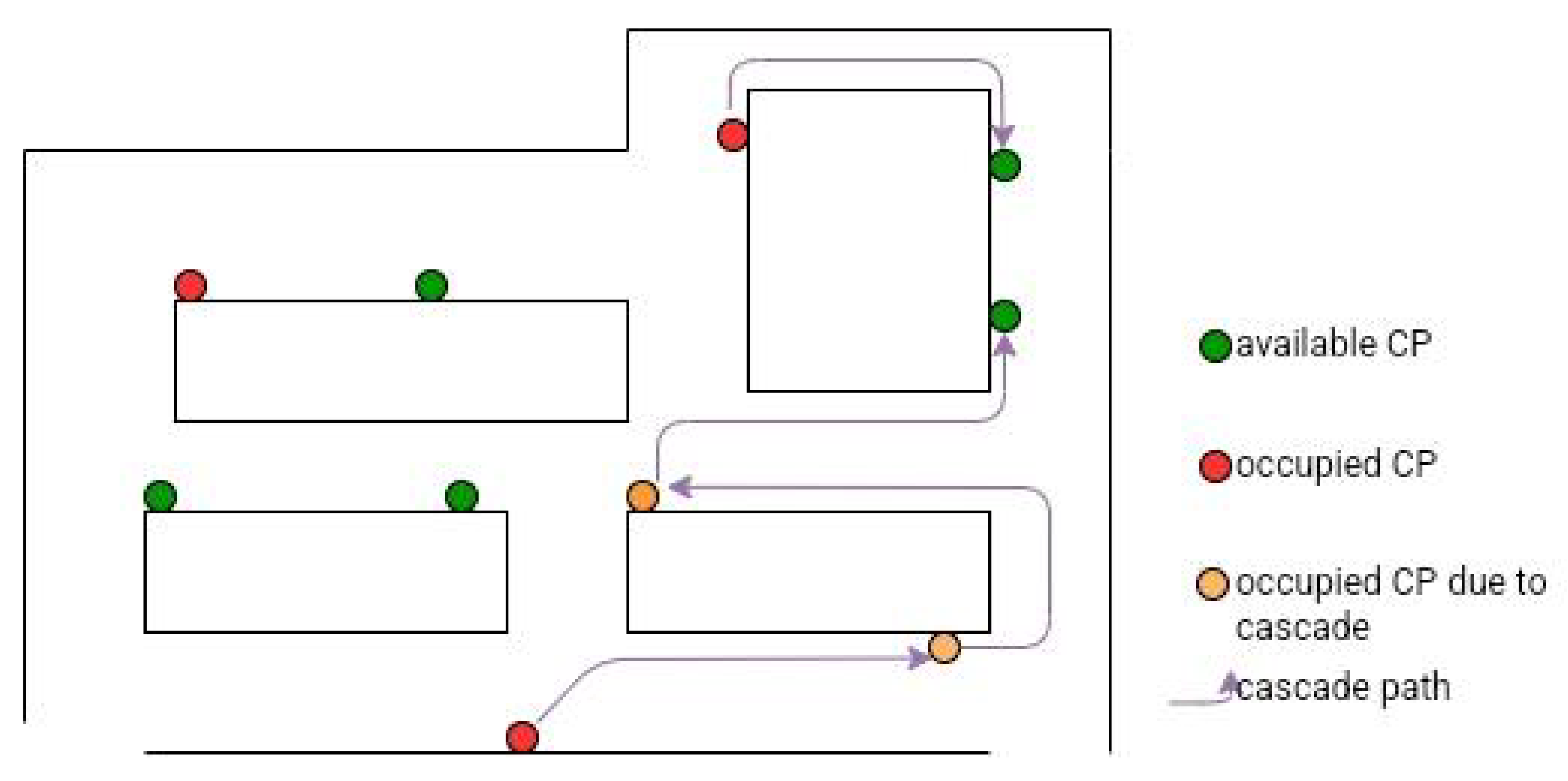
Earlier research on the vulnerability of charging infrastructure has shown that a disturbance in the system, either a malfunctioning or unexpectedly occupied charging station, can cause a cascade of failures in the system (illustrated in
Figure 3) [
18]. Simulation models of EV user charging behavior have shown that the number of failed connection attempts to an EV system is sensitive to changes in the number of users for a given size of the infrastructure under relaxed circumstances (limited users and without noise) [
71].
3.5. Self-Organisation
A typical property of a CS is the lack of central control. This means that the system is self-organized in a bottom-up manner [
22]. A CA, as a whole, may become more organized over time, without any external forces on the system [
72,
73]. In such a state, the system organized itself such that the size of the cascade of a propagated perturbation displayed a power-law distribution [
74,
75,
76]. This implies that many perturbations cause little impact, but some cause massive system scale impacts. This CS aspect has been found in public infrastructures, such as the electricity network [
75].
We expect an EV system self-organizes in two aspects: (i) network components with robustness or vulnerability, similar to critical infrastructures, and (ii) segregation of CPs for dedicated EV user types. First, for the EV system, we expect that the system grows towards a dense network of CPs, EV users, and their interconnected relations. From this, we expect that both the number of detours will increase, as more pressure on the EV system leads to a larger number of failed connection attempts, as well as the number of diverted EV users to other CPs [
71]. In a dense network, we expect the distribution of the cascade length to move towards the SOC, as found in critical infrastructures. Second, we expect CPs in specific areas to be used for specific user types that prefer high availability of CPs over location. As an example, EV users that are limitedly bound to charging locations (logistics, taxis, or overnight charging e-carsharing) will select CPs that have high availability when they arrive at their destination.
3.6. Non-Linearity
A non-linear system is one in which the output of a system does not scale linearly with the change of the input or parameter of the system [
43,
77]. In a non-linear system, the superposition principle is that the system state cannot be obtained by the addition of two solutions or one solution multiplied by a factor. As such, scaling the size of such a system may result in different regimes of behavior at the micro and macro level, without changing the properties of entities at the micro level.
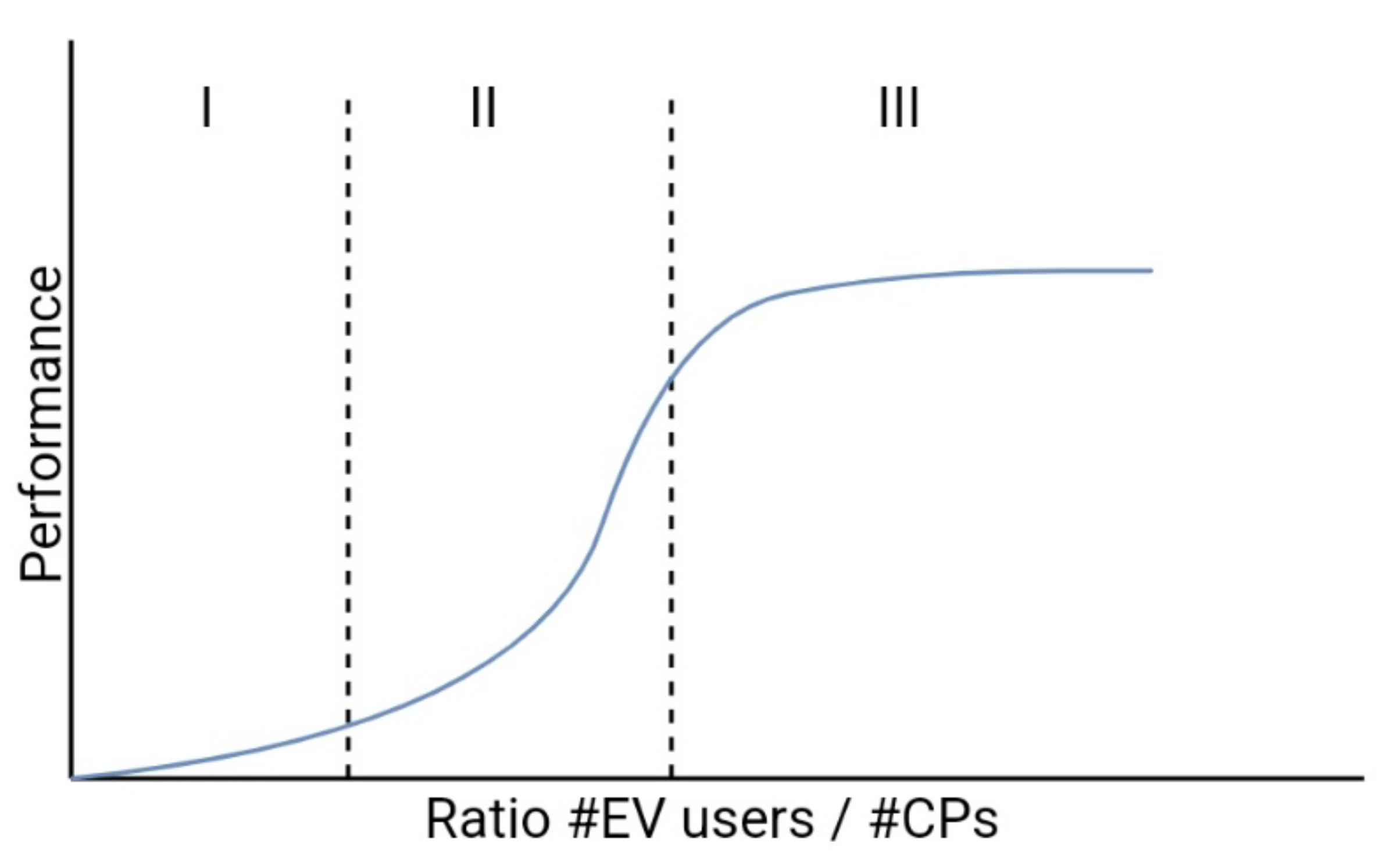
Recent literature has found non-linearity when scaling the EV system in the supply side, as well as in the ratio of supply versus demand. More specifically, three types of regimes may be present in the EV system during scale up: (i) a linear regime in the early stages, (ii) nonlinear increase of performance (due to economies of scale), and (iii) nonlinear decrease of performance (due to competition effects) (as illustrated in
Figure 4). Regarding the scaling of the supply side, we see economies of scale, due to network formation, as the density of the charging network increases [
50,
78]. As the network density increases, these economies of scale lead to a marginal decrease of the performance metrics and exponential increase of inconvenience for EV users, due to CP occupancy. Recent research, that involved the addition of new EV users to an existing charging infrastructure, revealed that performance metrics growth marginally decreased towards a maximum, while failed connection attempts increased exponentially [
71].
Moreover, in the case of public charging infrastructure, there exists EV users of different user types, using the same charging stations, which may lead to unexpected results for key performance indicators (KPIs) as the system scales [
11,
49].
3.7. Path Depencency
The development of a system’s behavior over time is said to be path-dependent. This refers to the fact that initial conditions and ensuing interactions between elements determine that certain development pathways are locked [
79]. As such, currently evolving and interacting components and stakeholders, on different levels, play an important role in the system’s future state [
30]. An example of path dependency is found in health care systems. The legacy of historical structures and stakeholders is the reason that it is difficult to reform the health care system from its current financial structure to another [
43].
Similarly, in the EV systems worldwide, we see different versions of initial conditions, due to the local context: metropolitan areas with public parking locations focus strongly on public AC charging, whereas areas with more private parking locations focus on DC and private charging. Once the system is rolled out, it may be difficult for policy makers to change the local EV system from pure AC public charging to DC only charging and vice versa, due to all the interactions of charging infrastructure with users and other systems. Therefore, the mix in charging infrastructure technologies in a metropolitan area is likely to be more dependent on the initial roll-out strategy [
23] than subsequent developments. This emphasizes the necessity of future scenario planning for policy makers.
On a local scale, path dependency is present, as the deployment of new CPs has been found to lead to local uptake of additional EV users [
1,
80]. This feedback loop implies that the current spatial distribution of EV users may be causally related to the developed infrastructure over time. This implies that any decision for CP deployment deviating from current location may have led to a different layout, in terms of spatial EV and CP distribution.
3.8. Phase Transitions
Phase transitions are large changes in macro behavior or a system that are due to minimal changes [
43]. Phase transitions occur either suddenly or gradually when changing elements reach a critical point. In some cases, there are early warning signals in the system, such as a critical slowing of system metrics, that announce an upcoming tipping point [
81]. In many cases, it is desirable to avoid phase transitions, as the new state of the system may behave differently or react differently to policy interventions [
58]. In systems of supply and demand, phase transitions have been found in collapsing stock markets, sudden traffic jams, or social networks [
82]. While models have provided insight into, and measurement of, the drivers of transitions [
82,
83,
84], it is still difficult to predict these in chaotic systems [
85].
For the EV system, not only will the number of EVs and charging points grow in the near future, but we also expect changes in EV user behavior, leading to different aggregate patterns of system performance for four reasons. First, the improved range of new EVs is expected to influence the behavior of users, as high battery full electric EVs (FEV) are expected to show different charging behavior than plugin hybrid EVs (PHEVs) [
6,
86]. Second, the ongoing increase of EV users will lead to new types of user groups adopting the EVs as their primary transport. While during the first years, EV adoption was particularly attributed to early innovation adopters curious about new technologies and driven by environmental consciousness, the new growth is expected to contain the early majority that is driven by economic motivations and had high expectations towards CP availability. This sets new requirements for charging infrastructure and corresponds to the idea that technology maturity affects usage behavior, as seen in other fields of innovation [
87]. A third reason is that not only the user groups will differ, but also other types of modalities (e.g., vans and heavy-duty trucks) will adopt electric drivetrains [
88]. Finally, an increased number of users will also inevitably lead to an increased number of non-trivial, user-user interactions in the system.
4. Analyzing the Complexity of the EV System
So far, we have described the EV system as a social supply–demand system (SSDS), and we have projected the properties of complexity on the EV system. Regarding this complexity, we pointed to (i) limited predictability of behavior due to interactions, (ii) issues of scaling non-linearly, and (iii) existence of non-measurable effects (not measurable in transactional data). Not all SDSSs display complex behavior, and some configurations of SSDSs may push the system towards more complex behavior. Moreover, the complexity of a system is a gradual scale of factors that drive the complex behavior, rather than a true/false value.
In this section, we elaborate on the how to analyze the complexity of the EV system. We try to reason about certain properties and ratios in the system that are drivers for complexity. We see different configurations of EV systems in different types of geographic areas (e.g., rural or metropolitan areas), with different charging modes as dominant [
89], i.e., AC home charging, public DC fast charging, semi-public AC charging, or AC public charging. We ask ourselves where the EV system and particularly metropolitan AC charging fits on the scale of complexity. Insight into the current state of complexity, and its drivers of the EV system, provides us insight into how this complexity is going to change over time. Will the current challenges of the EV system be relevant in five years, and what is the future relevance of the current research outcomes?
4.1. How Complex Is the EV System?
The rate of complexity in a system has been the subject of many studies [
40,
90,
91]. People have tried to understand quantitative measures of complexity by using quantitative methods related to physics, information theory, or computational science [
90,
92,
93]. Researchers, however, have experienced several difficulties with these metrics, including (i) computational challenges, (ii) limited descriptive meaning, and (iii) limited comparability between models or systems (e.g., [
90,
92,
93]).
In practice, there is only limited information of elements in the system available. Available data may include individual transactions between supply and demand side elements (e.g., charging transactions), but not social interactions between either side of the system. In cases of health care or education, additional information about waiting lists may be present. Nonetheless, the set of available data are not sufficient to exactly measure the complexity of the system. Moreover, metrics on aggregate that are based on transaction data level may not capture aspects of locality- and time-dependent use patterns. Therefore, rather than calculating a precise number for the complexity of the EV system, we present ratios that indicate and qualify its complexity [
22,
94].
Based on the abstraction of a public charging infrastructure, we observe three conditions for the ratios that determine complexity of behavior in the system. We determine equations for three ratios, based on the elements defined from our description of a social supply–demand system.
The first ratio describes the rate of competition, in terms of the necessity of sharing resources using overlapping sets of CPs, selected by EV users, and relates to the common-resource pool (CPR). The second describes pressure on the system, related to the demand and service rates, and uses the concept of queueing theory. The third ration describes how the impact of a single transaction on other transactions spreads within the timeframe and vicinity of the transactions. The ratios allow us to reason about the rate of complexity of extreme cases. For instance, why are AC public chargers complex and DC fast chargers (similar to current petrol stations model) or AC home chargers not complex?
4.1.1. Ratio 1: Necessity of Sharing Resources
The first ratio relates to CPR literature and involves the necessity of sharing resources
, by users
, in a set of transactions
. This ratio builds upon the clustering metric for bipartite graphs [
95]. For the first ratio, we consider the overlapping competition of users over access points, in relation to the union set of access points to choose from. The more competition there is for every transaction in the larger part of the system, the more complex interactions can be expected. We see that the number of the demand side elements is much larger than its supply side counterpart, such that, at any given time (
), users may select CPs that are occupied. A poor system level approximation would be
, but this does not include locality of EV users’ activity patterns.
In
Section 2.4, we have described that each user
makes decisions at some frequency (
) (transaction per time unit) for a transaction (
) at resource (
). Most systems are partially observable, which means that each transaction decision a limited set of resources is visible
For each
within the user transactions, a subset of resources (
) will be preferred, where
.
We, therefore, setup the Ratio
1, in line with node clustering metrics in bipartite graphs [
96]. First, we set a timeframe (
) to
, with a transaction set of
. We define
as the set of all pairs of transactions
from two different users
, where
at their given location
, based on the location of the resource access point. We consider the set of considered resources
of users and observable resources per location
We calculate Ratio
1 as follows:
With this first ratio, we relate potential competition over the alternatives to both time and space and normalize this value over the size of the set of all possible transactions. This first ratio may be calculated on a system level, but also locally (e.g., neighborhood or a connected set of alternative CPs). For the case of home charging, we see that the value of Ratio
1 approaches 0 as (i)
is zero, in most cases, since each user has its own CP (
Figure 5a). On the other hand, for DC fast charging, all users may potentially select any of the available outlets at arrival, leading to a value close to 1 (
Figure 5c). For public charging infrastructure, we see that the set of overlapping
is smaller than
, which leads to a value significantly lower than 1 and higher than 0. For semi-public charging, we expect values close to DC fast charging, since both
and
. We expect that complexity decreases at the limits of this ratio (0,1).
4.1.2. Ratio 2: Probabilities of Queuing
The second ratio (Ratio
2) specifically focuses on the complexity of behavior in the system, related to the time aspect (e.g., service rate of supply and demand). This ratio builds upon the concept of supply and demand rates, which has been studied in queueing theory [
97]. In queueing theory, the ratio between
determines the probability of a queue’s existence. In this equation,
is the arrival process, assumed to be a Poisson distribution
(defined in our SSDS as
), and
is the exponentially distributed service time (
in our SSDS) [
97]. The literature on DC fast charging infrastructure has modeled outlets as a multi-server network queue [
98,
99]. Yet, for AC public charging, the following aspects make queuing models complex in highly occupied systems [
97]: (i)
is not a property of the outlet alone, as it is related to parking behavior, rather than transactions size; (ii) EV users have shown to be strongly habitual, causing multi-modal Gaussian arrival patterns, rather per
[
3]; and (iii) when EV users arrive at a location, they have individual preferences for
, even if they overlap in locality.
In line with network queueing models, we define Ratio2 as the duration time of a transaction divided by the mean time between arrivals at . To take locality into account, we average over each set of local observable resources , rather than over the whole system at once (e.g., ).
First, we consider
as the set of all
in the system. For each
, we calculate the local
and average over the set of resources in
, and we call this
. Ratio
2 is, therefore, calculated as follows:
The value of
is calculated by using the following steps. First, we consider the union set of transactions at all access points within
, where
as
and
. From the tuple
=
we use the connection duration
as
; information in tuple
allows us to define
as the interval between two consecutive transactions
,
, using
from
and
from
. In
Figure 6, this is displayed as time between sessions. We can now calculate
.
In
Figure 6, we provide a schematic overview of how charging sessions are distributed over time. For DC fast charging, we see that the connection duration
is short, due to the high transaction speed and
varies during the day. Variation of
(
Figure 6) is related to traffic intensity (peaks in the morning and evening). For a private home, the charging sessions are long (e.g., overnight charging ~ 14 h), and inter-arrival times may be 24 −
, in the case of one EV per CP. For both semi-public and public AC charging, the sessions are also long. Thus, many arrivals may potentially take place during a connection time within the local
. For semi-public charging, we expect the values to depend on the specific function of the semi-public location (e.g., garage in dwellings may be different than park-and-ride locations). For public charging, we expect different values of
, based on the local population composition.
Regarding future values, we expect per user to decrease over time, as battery sizes increase. Yet, we expect to not change dramatically over time, as charging behavior often involves parking activities. As such, we expect limited changes to Ratio2 and, consequently, limited changes in the complexity for AC public charging.
4.1.3. Ratio 3: Impact of Transactions on Others
The third ratio relates to the spread of the impact of a single transaction on other transactions, as found in the literature on cascading perturbations [
36,
100]. A decision of a user to make a transaction may affect other users’ transactions at the CPs in the vicinity; this, in turn, may have a knock-on effect on other transactions. The spread of impact cannot be measured from the transactions, since each transaction is a successful connection attempt, resulting in an as-is state that includes the knock-on effect. We, therefore, define this ratio by estimating the effect of taking an alternative decision (over all alternative resource outlets) to other users’ ability to connect to their preferred resource outlet. We use an iterative approach, as the alternative decision of the first user may lead to a cascade of successive alternative decisions of other users. The volume of the spread over all alternatives normalized against the set of geospatial alternatives (
gives us an indication of the average spread per transaction [
101]. We note that, similar to other complex infrastructures, the calculation of these metrics required simulation models, as it is not feasible to measure this value in practice [
102].
We setup Ratio
3, in line with literature on cascading failures, as follows [
103]. In line with the other ratios, we set a timeframe (
) to
for a transaction subset of
. For
, we initiate the set
, which we fill with transactions
affected by the alternative decisions that
may have made for transaction
and initiate
as the set of alternative
, which we have taken into consideration during calculation. We iteratively perform the following calculations.
- (1)
of we regard as the set of alternatives minus the already considered , in using ;
- (2)
For all , we add the set of affected transactions at during the interval to ;
- (3)
For , we return to (1), while adding transactions to the initial until .
Using this depth-first search, we calculate the ratio using Equation (3).
In
Figure 7, an illustration is provided of the spread for several types of charging infrastructure. The arrows in
Figure 7 indicate first second and third tear spread. For DC fast charging, the spread involves first tear effects to all CPs, as the effect of one decision is short, due to the short transaction connection, as well as the fact that
~
. We, thus, expect Ratio
3 to be low for DC fast charging. For private home charging, the spread takes, as a maximum, the value of the number of EVs that share the home charging CPs. The Ratio
3 value is expected to be between 0 and 1. For semi-public charging, we also expect this value to be between 0 and 1. For the mature public charging infrastructure, we expect this value to be above 1 [
104].
4.2. Conclusions on Complex System Ratios
In this section, we have defined three ratios that help to identify the complexity of behavior in the EV system as a social supply–demand system. The metrics presented here require simulation models (e.g., network simulation) to approach the exact values. While we did not precisely determine the three values, we were able to compare public AC charging with DC fast charging and private home charging. Our estimation showed that the values for public AC charging significantly differ from the other two charging types. Based on a qualitative assessment on the three ratios, we conclude that public CI can be characterized as complex, given that, (i) in dense networks, there is a lot of competition for scarce resources, (ii) likely queuing, and (iii) long cascades of perturbations.
Based on the variables that are present in the three equations, we can also estimate whether the complexity of the system will change in the next two decades. For instance, will an increased charging speed and battery of DC charging make the current system redundant?
First, we see an increased battery size will lead to a reduced
and
, as well as an increased transaction size, leading to lower values of ratio 2 and 3 for both DC fast charging and AC public charging. For AC public charging, we do not expect the connection time
to be directly affected by the battery size, since connection durations are related to parking behavior [
56]. For DC charging, on the other hand, the ratios may reach values comparable to current petrol stations. Whether DC charging will grow towards the dominant charging mode cannot be answered by these ratios alone [
105], since market developments play a role, as well.
Second, we expect the charging infrastructure to mature as the size of user population, number of CPs, and number of transactions will increase. The set of pairs will increase exponentially as the system grows, but the effect is limited, as Ratio1 is normalized over all pairs. We expect and to increase as the density of the CPs increases. We also expect to decrease as more users have nearby subsets of options. We expect to increase as the set of alternatives grows. As such, we expect a slow decrease of Ratio1 over time and the complexity to slightly decrease. On the other hand, an increase of and may lead to an increase of Ratio3 and the spread of effects of alternative decisions. In the end, this may add to the complexity of the behavior in the system. We, therefore, expect that AC charging infrastructure (separate from its public DC counterpart) will remain within the complex regime.
5. Analyzing Interactions and Performance of Complex Systems
Measuring the performance using system metrics of a complex system (CS) helps to define, implement, and monitor the interventions that increase the effective deployment of resources and evoke efficient use of the system [
106,
107,
108]. A prerequisite is the availability of at least transactional data that allows for the derivation of measures for both the resource and user side. In various systems, transactional data are collected at the providers of resources (e.g., health care providers or schools) or by individuals (e.g., stock exchange records and GPS navigation systems).
The problem with measuring CS performance is that, typically, the metrics that matter emerge from bottom-up interactions. The metrics measure the results of the interactions, not the interactions themselves. This means that CS properties, such as feedback loops or user intentions, that do not result in a transaction are limitedly captured by transactional data. In an ideal world, one would have complete information of the system that is not only the result of behavioral intentions but also the intentions themselves, as well as the user experiences of the intentions and interactions between the intentions. For instance, measuring the market cap of a stock, without the lending network or information on buyers’ intentions, makes difficult, if not impossible, to predict a stock crash [
109]. Therefore, to effectively intervene with the system, we also need understand the relation between performance and the underlying behavior of the system.
In the next paragraphs, we describe systemic metrics, focusing on the interactions between elements in the system and methods to model the system, in order to analyze the interactions.
5.1. Systemic Metrics for Charging Infrastructure
The EV system contains non-trivial dynamics, due to interactions between users and charging points, such as a user-user interaction (competition or collaboration). In contrast to system metrics that focus on performance, the systemic metrics quantify the interactions between elements in the system. To analyze these interactions, we consider the system from a complex networks perspective by using (i) network graphs from geospatial data and (ii) bipartite graphs generated from charging data (mappings between supply and demand) [
95,
96,
110,
111]. Typical metrics, from both the supply and demand side, can be measured, and interactions can be inferred between elements (e.g., user-user) in the system.
First, using the geospatial information, a network can be defined as consisting of vertices () and edges (), where and edge is a connection between two elements of V, defined according to specific thresholds. An edge between and , where , exists if a distance () exists less than a threshold (). The distance () may be defined by time, such as driving time, walking time, space driving, walking distance, or distance as the crow flies. The edge () represents that, for , there is a relevant alternative ((relevant according, based on < ). Varying the < condition may help to adjust the network to the maturity of the infrastructure.
From this network, several metrics can be distilled that may help policy makers to make rollout decisions. First, the degree distribution, i.e., the distribution of the number of connections per CP, helps policy makers to reinforce the geospatial network at locations where the number of alternatives is limited [
102]. Second, the number and size of connected components (sub-networks) within the large infrastructure may help to grow the EV system as a network. For instance, a growing network is considered more robust if the size of the largest component, relative to the total network, is kept constant [
50,
73,
112]. This can be achieved if policy makers select CP locations that interconnect the subnetworks.
The second network type is the bipartite graph. This graph is a triplet
, where each edge
is a connection between one top (demand) and bottom (supply) edge and derived from the set of transactions. Bipartite graphs have been used extensively in computational ecology to model natural plant-pollinator systems [
42,
66]. The bipartite network has been used to solve allocation problems [
96,
113] and model the effects of invasive species on current population and, in our study, the EV adoption of specific EV user types [
35,
66]. This network has also been used to quantify the risk of system collapse [
42] and detect a system’s potentially unstable configurations [
114,
115]. At a detailed level, the detection of bicliques (fully connected subsets of upper and lower elements) helps to reveal the effects of local competition for resources.
Simple metrics for bipartite graphs contain the average degree of a top or bottom node
or
or the density of the top
or bottom
of the bipartite graph [
116,
117]. As with the geospatial metrics, these metrics may help to strengthen the CP network at specific locations. The redundancy coefficient captures the impact of removing node
on its
connections, as defined by
of node
[
118]. This metric allows us to identify spots in the network with an excess of supply. The average path length over the bipartite components may help to identify regions where the effects of decision making of one EV user, in comparison to others (similar to Ratio
3), is high.
The bipartite network also allows us to project relations between elements of or , based on existing edges. In the context of charging infrastructure, the -projection explains the relation between charging points, based on overlapping sets of EV users, and the -projection describes the relation between EV users, based on the overlapping sets of charging points. Both projections may be conditioned on time ()-specific aspects, such as daytime or overnight charging. The projections may also be created as weighted graphs by using the number of transactions for the weights. Contrary to the geospatial network, the -projection describes the actual used CPs as alternatives. This projection may even include nodes that are not near each other, but still used by the same users (e.g., fast charging and CPs at shopping malls).
Both projections may help to quantify emerging CS, such as competition or collaboration [
119]. Metrics for the projections that are interesting for policy makers contain the aforementioned graph metrics. Additionally, for
-projection (CP to CP network) the following metrics are specifically interesting. For each component of the
-projection, the eccentricity (the maximum shortest path between two nodes) gives an estimation of the largest possible cascading failure in that component. For the
-projection (user to user network), clique detection and local density of a specific component may help to determine which sections of the network to support with extra CPs.
5.2. Modeling Charging Infrastructure as Complex System
Complex systems (CSs) are notoriously difficult to accurately model [
120,
121]. The challenge is often that there is no full behavioral information available in the system, since behavior measurable at an aggregate level is typically developed bottom-up. In the case of the EV system, we have a set of information that contains transactions of users at specific outlets, which, by definition, contains only the results of successful connection attempts [
7]. As such, the failed connection attempts, as part of the interactions, are, by definition, not present in these data. The solution is to build models that generate simulated behavior that can be validated with the available information [
122].
A common method to model CS from a bottom-up approach is agent-based modeling (ABMs) [
123,
124,
125]. In ABM, each agent (i.e., EV user) acts autonomously, according to its individual assigned behavior [
126]. The agent interacts with other agents within an environment (e.g., a network of charging points), from which it adapts or learns its behavior [
126]. A concern of ABM use is that the outcomes of ABM simulations provide qualitative answers to what-if questions, rather than a precise description of a system’s future state [
127,
128]. A critical note is that the quality of simulation outcomes may be limited, without available validated (data based) descriptions of micro-level behavior [
124,
129]. Data driven calibration and validation of ABMs have been the subject of recent studies, as more data has become available [
129,
130].
Bonabeau [
124] summarizes five conditions for a system, for which it is useful to model using ABMs. First, the interactions between agents are complex, nonlinear, discontinuous, or discrete, as described in
Section 3. We expect that the interactions between EV users, due to CP occupation, results in nonlinear effects of adaptation, shifting preferences, cascades, or strategic charging behavior, in order to avoid competition between users. Second, Bonabeau states that the space dimension must be crucial for the agents’ behavior, which corresponds with our abstraction of the EV system as a social supply–demand system (described in
Section 2). Third, ABMs are considered a suitable tool if the population of agents is heterogeneous, as each individual agent has its specific behavior. In the EV system, we see that, in both time and space, each agent has a specific charging behavior (i.e., arrival time and CP preferences). Moreover, in a metropolitan area, with its diverse population, we also expect different user types with differentiated behavior (e.g., residents, taxis, and car sharing EVs). This presence of various types of users fits with the fourth condition that the topology of the interactions is heterogeneous and complex. Finally, the ABMs are specifically suitable to simulate systems in which complex behavior, such as learning and adaptation, play a role. This is in line with our expectations of EV user behavior.
5.3. Proposed Model for Analyzing Charging Infrastructure as Complex System
Based on (i) our abstraction of charging infrastructure as a complex system and (ii) the set of complex systems properties, we suggest including the following features in ABMs for the EV system. First, we propose to include (i) the charging network of CPs, complemented by set of relevant alternatives per CP; (ii) EV users with a feature set, as described in 2.3, with special attention to the battery size (
), charging speed (
), and charging behavior, in terms of frequency (
), quantity (
), and quality (
). Second, we propose to include rules based on preferences (
) (as shown in
Figure 2), in order to allow EV users to learn and adapt to interactions. These rules should include (a) the search for alternative CPs, in order to allow for demand side network effects; (b) strategic deviation from arrival preferences to avoid competition; or (c) rules for collaboration with other EV users. Additionally, the relation between the charging frequency (
), battery size (
), and charging speed (
can be modeled, in order to allow to phase transitions in simulations. Third, policy makers and additional EV uptake may be present in an ABM, as special type of agent, in order to allow to reveal feedback loops and path dependency in deployment strategies.
With this setup, we propose to simulate scenarios for different service rates, EV user population compositions (in terms of number of users and different battery capacities (hence, different charging behavior)), and different charging layouts. As part of the analysis, we propose to measure competition and collaboration using systemic metrics, network robustness, and non-linear scaling effects.
6. Discussion and Implications for Policy Makers and Research
Policy makers play a key role in the EV system, particularly in the deployment of public charging infrastructure. Their degree of freedom is limited in choices, in regard to when and where to deploy and what type of charging infrastructure to deploy, while the effects of decisions are large. In this research, we have made a case that (i) charging infrastructure can be abstracted as a social supply–demand system (SSDS), similar to other systems; (ii) charging infrastructure is in a complex system, based on several ratios; and (iii) complex systems may add to better understanding of the performance of charging infrastructure. From this, we advocate that the use of complex systems and ABMs, as a modelling tool, may support policy makers in making more robust solutions for the anticipated exponential growth of EVs.
6.1. Implications for Policy Makers
Based on our research, we see the following four implications for policy makers. First, based on the ratios derived from our general abstraction, we also see that the rate of complexity depends on the type of charging deployed. Therefore, to reduce complexity, policy makers need to develop a strategy that consists of a base public AC charging infrastructure, combined with inner city semi-public and DC charging.
Second, policy makers may consider specific complex system properties, while (i) deploying charging infrastructure or (ii) implementing interventions. Being conscious of the learning effects and feedback loops of EV users may be key to tailored roll-out strategies for local circumstances. For instance, based on charging data analysis, policy makers may find patterns of EV user adaptation to local competition or collaboration. Robustness and vulnerability are essential elements of complex systems; in the context of charging infrastructure, they relate to convenience of EV users [
18]. It is known that the higher utilization of a system leads to higher tension and criticality of the system. While policy makers tend to optimize on performance, in terms of utilization of charging points, a balance between performance and robustness may lead to a higher total system convenience.
Roll-out strategies specifically focused on decreasing the network vulnerability may lead to an increased convenience for EV users, while having a marginal impact on efficiency. While it is difficult to generalize learnings on path dependency, it is still an important factor that policy makers should be aware of. Both in research, as well as in practice, there seems to be two mutually exclusive paradigms for charging point technologies: AC Level 2 charging or DC fast charging. Deploying charging infrastructure, as a portfolio of several technologies, may avoid certain paths becoming excluded.
Third, we have learned that systemic metrics (key performance metrics) do not fully capture information on interactions. Based on our research, we suggest taking into account systemic metrics for monitoring the system. Visualization of the charging network of relevant alternatives may help to select locations to reinforce the network. The use of bipartite projections may help to search for high competition areas.
Fourth, policy makers should embrace the use of simulation models, in addition to using data analysis. Until now, most deployment strategies have been based either on the actual demand of EV users or expected demand at strategic locations near points of interests (POIs). This approach has proven to be successful during the first phase of deployment; however, for the system’s future growth, this approach may not be the most optimal. For example, economies of scale may arise, due to network density or user interaction, and lead to counter intuitive complex phenomena. Using agent-based models to test deployment strategies or gain insight into complex interactions in the system may help policy makers to improve deployment strategies.
6.2. Implications for Research
Based on our results, we can define two types of implications: (i) the application of complex systems may be scientifically interesting to apply to the EV system; and (ii) the results from the EV system may be relevant for researchers of other systems.
Regarding our first point, we believe it would be beneficial to put research questions commonly found in complex systems theory, in the context of EV charging. An interesting scientific challenge is to spot the early warning signals of upcoming regime changes in charging behavior. In close relation to that, growth towards self-organized criticality of a system, where the effect of perturbations follows the power law distribution, has gained much attention in the scientific community. These phenomena are linked to systems that follow rules of natural phenomena. It may be interesting to see in what sense the EV system is led by rules that also apply to natural systems, rather than attribution performance to user behavior.
The literature on modelling complex systems using ABM models or network models may help advance our understanding of the EV system. ABMs rely on the quality of the underlying behavioral model. Recent advances in ABM methodologies include the use of behavioral data as a starting point. Data-driven rules for agents may be of particular interest for EV research, since EV maturity tends to differ worldwide. Sharing the rules themselves, rather than the underlying data, may avoid issues of privacy infringement, as well. In addition, ABMs are difficult to reproduce; it would be beneficial to share ABM code and documentation online (e.g., GitHub) for research purposes.
Regarding the complex network analysis of charging infrastructure, it would be scientifically interesting to compare the resilience of the networks within metropolitan areas worldwide, in relation to performance, user behavior, and perceived user convenience. This may also help us to better understand path dependency, in the context of charging infrastructure. Research in path dependency may create a set of generalized insights, based upon the different contexts of metropolitan areas. These insights would provide a better understanding of the complex tasks of deploying any new kind of infrastructure.
Finally, while this research focuses on the EV system as a social supply–demand system, the insights that we have gained can be beneficial for other systems with a similar rate of complexity. Many complex systems are difficult to model, due to limited availability of detailed behavioral data. Yet, charging data, as well as additional data from surveys or driving, are available for research to gain a better understanding of resource selection behavior. The development of a set of behavioral models, based on detailed data, may not only help EV research, but may also benefit other research.


