Compressed Driving Cycles Using Markov Chains for Vehicle Powertrain Design

Abstract

In recent years, topics of digitalisation, urbanisation and sustainability are shaping future developments in the automotive industry and pose new challenges to the individual areas of vehicle development. In the design and simulation of multiple components in the vehicle, especially in powertrain, generically generated driving cycles play an important role since they reflect representative user behavior. Nowadays, driving cycles are mainly associated with the worldwide fuel consumption and emission tests, but they are nevertheless used in many fields of vehicle development. A design based on the currently used consumption and emission cycles proves to be unsuitable, especially for electric vehicles. This is reflected in the current discussion about the large discrepancy between the driving ranges achieved when using emission cycles and those under real driving conditions. In order to minimize the energy consumption of a vehicle, the main requirement is a good efficiency of the electric machine. Here, not the maximum efficiency of the machine is decisive, but the averaged overall system efficiency during real driving behavior. The electric machine must therefore be designed for the driving cycle. To optimize the use of electric machines in the future, the actual power requirements of future vehicle models must first be determined. In the course of this paper, a compressed vehicle class specific driving cycle will be created based on real driving data using Markov chains, which can be used for powertrain dimensioning.

1. Introduction

The anticipation of user behavior enables a performance related design of the entire powertrain. Driving cycles that are intended to represent customer behavior regarding powertrain usage are one possibility. The major difficulty here is to represent customer behavior through driving cycles based on a wide variety of driving conditions [1]. Current conventional driving cycles, such as the Worldwide Harmonized Light-Duty Vehicle Test Cycle (WLTC), are used for type approval and to determine fuel consumption and exhaust emissions [2]. However, there are no specific driving cycles for the design and dimensioning of individual powertrain components. The WLTC is not a satisfactory solution for this, since driver characteristics and driving preferences are not taken into account [3] (p. 24). However, this consideration is of great importance, for example, when designing a small car in direct comparison to a sports car. Although a distinction is made between three different vehicle classes for the use of the WLTC, if one takes into account that almost all vehicles sold in the EU fall into just one of these classes, it is not possible to speak of a differentiated consideration [4].

The knowledge that the WLTC does not represent driving behaviour in Germany and throughout Europe realistically clearly underestimates consumption values and thus does not place appropriate demands on a vehicle [5], and shows the necessity of new realistic driving cycles for the design and dimensioning of future powertrains in research environment. Therefore, different methods for the design of driving cycles are presented in this paper. Subsequently, a new methodology is shown which makes it possible to generate vehicle class-specific driving cycles by a parametric cycle construction approach that reflect the real vehicle usage and can be used for the dimensioning of powertrain components for future vehicle concepts.

2. State of the Art/Conventional Driving Cycles: Methodologies and Qualification

The basic objective in the development of driving cycles is to reproduce customer driving behavior with regard to the vehicle use. Influencing factors such as traffic conditions and different driving characteristics make this task difficult [1]. Many current methods for driving cycle design shown below were developed with the aim of determining local emissions more precisely [6,7].

2.1. Methods for Cycle Design Based on General Driving Segments

The microtrips-based methodology divides a driving profile into so-called microtrips and was presented by AUSTIN et al. in 1993 [7]. A microtrip is defined as the journey between two stops with an initial idle phase [7] (p. 113). Each of these microtrips is characterized by different parameters, such as the speed acceleration frequency distribution (SAFD). The cycle is then constructed by concatenating these microtrips. In doing so, as many microtrips of the duration t_trip are concatenated until the desired cycle time t_cycle is reached. AUSTIN suggests three methods for concatenating the microtrips [7] (p. 116). In addition to the random selection of a microtrip from the available pool of trips (Random), that microtrip can also be combined so that the target values of the driving cycle, such as the Watson plot, are reached as well as possible (Best Incremental). A hybrid approach combines the two methods for chaining microtrips [7] (p. 117). From the set of driving cycle candidates generated, the one whose distribution of acceleration and speed is most similar to that of the real driving data set is selected [7] (p. 116).

A similar procedure is presented in the segment-based method [8] (p. 197). In contrast to the subdivision into microtrips, the driving data is divided into driving segments which are characterized by different road types, traffic conditions or speeds [9] (p. 2). The speed at the beginning and end of a driving segment is therefore not necessarily zero. This must be taken into account when linking these segments.

The procedure of cycle construction based on pattern classification is also derived from the Microtrip-based method. The methodology was developed by ANDRÉ for the construction of the ARTEMIS cycles, which are used for the more precise determination of the emission [10]. The segmentation of the driving data is done using two components. First, a description of the current driving condition is derived from the driving data. Then, a description of the vehicle usage is extracted. ANDRÉ uses the speed profile to describe the driving condition. For this purpose, a real trip is divided into kinematic segments of homogeneous size. Based on different characteristics, these segments can be classified into 12 driving conditions. Each recorded trip is thus described by segments of these driving conditions. On a macroscopic level, a distinction is made between urban, rural and motorway driving [10]. The aim of the following cycle construction is to simulate the different driving areas with regard to their structure and chronology of driving conditions. A driving cycle for a driving area is generally composed of representative segments of the respective driving conditions. For this purpose, ANDRÉ defines a pattern and a structure for cycle construction of each area. This structure includes the driving conditions that occur and the relative proportions of the segments of these conditions. Furthermore, the sequence of driving conditions is derived from the observed probabilities of the respective driving area and anchored in the structure. The structure thus provides the framework and, together with the driving segments, produces a representative cycle.

2.2. State-Based Design of Driving Cycles

The procedures shown so far are based on the method shown by AUSTIN. LIN and NIEMEIER are presenting a procedure that is detached from this procedure, also with the aim of a real driving cycle for determining emissions [6]. The underlying assumption of this method, that the speed at timestep t_i depends on the speed at timestep t_i−1 with variable timestep size, allows the mapping of a driving cycle using a Markov process [6].

Markov chains model random processes in which the state transitions occur with given probabilities independent of the previous history [11] (p. 219). Mathematically, a Markov chain is defined as follows [12] (p. 100):

$$\mathrm{P}\left({\mathrm{X}}_{\mathrm{n}+1}={\mathrm{s}}_{\mathrm{j}}{|\mathrm{X}}_{\mathrm{n}}={\mathrm{s}}_{\mathrm{i}},{\mathrm{X}}_{\mathrm{n}-1}={\mathrm{s}}_{\mathrm{i}-1},\dots \right)=\mathrm{P}\left({\mathrm{X}}_{\mathrm{n}+1}={\mathrm{s}}_{\mathrm{j}}{|\mathrm{X}}_{\mathrm{n}}={\mathrm{s}}_{\mathrm{i}}\right)={\mathrm{P}}_{\mathrm{i},\mathrm{j}}$$

(1)

The entries of the so-called transition matrix P represent the transition probabilities. P_(i,j) represents the probability of being in state s_j at time t_(n+1), given that one is in state s_i at time t_n. More precisely, this is a 1st order Markov chain, where the next state depends only on the current state. A 2nd order Markov chain considers the last two states to select the next state.

When modelling a driving cycle with a Markov chain, the driving profiles of a real data set are therefore divided into driving states. The construction is then also carried out in four steps (Figure 1) [6]. After subdividing the speed profiles into driving states and classifying them into state classes, the transition probabilities are calculated in the second step based on the state transitions found [6]. In the third step, the construction of cycle candidates is carried out by a Markov chain with the previously calculated transition matrix. The final step corresponds to the procedures shown in above (Figure 1).

LIN and NIEMEIER use the acceleration profile for data segmentation in the first step. With a maximum likelihood estimation (MLE) approach, the velocity-time curve is divided into small physically meaningful sequences. The driving sequences are classified by applying the MLE approach again. The exact procedure can be found in [6]. Each class characterizes a driving state and thus also represents a possible state of the Markov process. According to LIN and NIEMEIER the concatenation of these states or the driving sequences of a state is done by assuming a 1st order Markov chain. For this purpose, the transition matrix is calculated using the identified states in a given data set [6].

$${\mathrm{P}}_{\mathrm{ij}}=\frac{{\mathrm{n}}_{\mathrm{ij}}}{{\sum }_{\mathrm{k}}{\mathrm{n}}_{\mathrm{ik}}}$$

(2)

The transition probability P_ij is then calculated as the quotient of the number n_ij of detected state transitions from state s_i to s_j and the number n_ik of all state transitions starting from state s_i.

If the travel data are segmented into states and the transition matrix is known, the cycle construction is carried out in four steps [6]. A start sequence with a duration of 120 s is selected so that the distribution of speed and acceleration of this sequence corresponds well with that of the entire data set. Based on the transition matrix, the next state is determined. For this purpose, LIN and NIEMEIER use a random generator weighted with the transition probabilities. In the third step, the most suitable segment from this state class is then selected. These steps are repeated until the desired cycle time is reached [6].

DAI, EISINGER and NIEMEIER extend this cycle construction methodology with a new segmentation methodology. In contrast to the state determination by MLE, the state’s acceleration, deceleration, cruising and idling are fixed as such [9]. The allocation of the movement points to one of the states is then carried out using four fixed parameters. An acceleration state is defined as a single moving point with an acceleration greater than a, or a sequence of duration t with an acceleration greater than a_t and an increase in speed of at least v over the duration t. A braking state is defined in the same way. The remaining driving points are classified as oscillating or idling states. For the optimal determination of the classification scheme (a, a_t, v, t) different targets are classified in a comprehensive evaluation parameter. The values determined by DAI, EISINGER and NIEMEIER can be taken from [9]. A driving profile segmented according to this methodology is shown in the Figure 2 below.

The construction of cycle candidates is also based on a 1st order Markov chain, but in a modified way. First, driving segments are formed from the different states in a separate Markov chain. The length of such a driving sequence is derived from the real driving data. A cycle candidate then consists of one or more such driving segments. The exact procedure can be taken from [9].

SCHWARZER and GHORBANI [13] show a methodology that also works with driving states, but is undefined with respect to the real driving data. The methodology was developed for the design of driving cycles for powertrain optimization. It is not necessary to have a database with recorded trips or trip sections that are combined to a cycle. Instead, the key parameters of a driving cycle can be described stochastically. The Driving Cycle Generation Tool (DCGT) is based on a nested modularity concept [13]. A driving cycle consists of several driving scenarios, which belong to one of the five categories stop and go, urban traffic, mixed traffic, interurban traffic, and highway driving. Each driving scenario is further composed of driving pulses, which are equivalent to a microtrip to AUSTIN. However, here a driving pulse is built up parametrically by the four known driving states acceleration, deceleration, cruising and idling. After an initial acceleration phase, a cruising section follows. Afterwards the vehicle is decelerated to a standstill (Figure 3). The modelled driving pulse ends with an idling sequence [13].

For the acceleration and braking sequence of a driving pulse, SCHWARZER and GHORBANI assume a linear course. The acceleration phase ends as soon as the cruising speed is reached. The braking phase also ends as soon as the vehicle is at a standstill. The modelling of a cruising sequence takes place within the DCGT by superimposed sine waves of different frequencies, which imply different driving conditions. The exact modelling can be found in [13]. The parameters required to calculate these driving pulse segments, such as the constant acceleration value for the acceleration segment, are represented by probability functions. These functions can be derived from real driving data or they can be freely defined [13]. In this way, driving pulses can also be generated which have not already been driven in real traffic. Increased vehicle loads can thus be synthetically specified. This makes the approach shown useful for stochastic optimization of powertrain components [13].

2.3. Limitations of the Previous Methodology

For the design of dimensioning-relevant driving cycles, a driving cycle must also be able to cause high vehicle loads, matched to the corresponding vehicle class. Criteria are derived from the set target image, which must be fulfilled by a cycle design methodology. A robust data segmentation, especially for different driving styles and vehicles, is an important requirement. A fully parametric cycle design is the central requirement. In order to be able to generate vehicle class-specific driving cycles, cycle characteristics such as maximum acceleration or maximum speed must be limited during driving cycle construction. A targeted intervention in the cycle design must be made possible here. Furthermore, it is assumed that the method enables a robust implementation and, as a result, maps a real driving behavior, which is relevant for powertrain dimensioning and at least allows the consideration of different vehicle classes. Based on these criteria, the methods shown for driving cycle design are generally judged to be unsuitable (Figure 4).

None of the methods shown meet all the criteria set for the construction of driving cycles with the target image being pursued. The method based on microtrips according to AUSTIN is characterized by a robust data segmentation. Depending on the data basis, however, the real driving behavior cannot be represented in compressed form. microtrips with a duration significantly longer than the desired cycle time can occur. An exclusion of this method for achieving the desired target image is due to the non-parameterizability of the cycle construction.

For the same reason, the pattern and segment-based approach is excluded here. The state-based method chains real driving segments to a driving cycle, analogous to the methods already mentioned. Furthermore, the segmentation of driving profiles into sequences of different states is not robust here. This is not critical if real sequences are linked together, but it is critical if characteristic values are to be derived from the segmented driving profiles for each driving state (details are shown below).

Only the method shown by SCHWARZER and GHORBANI is based on a parametric cycle construction [13]. The most important requirement is fulfilled here. However, due to its synthetic character, it does not reflect real driving behavior. Acceleration and braking processes are depicted in a highly simplified way and numerous driving situations of a real drive, such as transition areas from city to country driving, are not considered.

Therefore, in the following, a method is presented which is state based in its core, but has a robust data segmentation and allows a complete parameterization of the driving cycle design. In addition, a single Markov chain for the construction of a complete driving cycle is used here, which can map all driving areas and their transitions.

3. Enhanced Modal Cycle Construction (EMCC)

The construction of a driving cycle based on real driving data is implemented in four steps [6]. In the first step, the driving data are divided into sections. These driving segments can be characterized by different parameters, such as average speed or maximum speed. In the second step, a statistical analysis or a cluster procedure divides the driving sequences into classes based on their characterizing parameters. The construction of so-called cycle candidates takes place in the third step by concatenating these driving sequences. In the fourth step, a representative driving cycle is selected from the set of driving cycles using defined criteria.

3.1. Steps of Enhancement

For the calculation of a parametric driving profile the acceleration a_i is required at any time t_i. The velocity v_(i+1) of a next time t_(i+1) is then calculated from the acceleration a_i and the velocity v_i of the past time. The calculation of a driving profile is therefore carried out iteratively for any points in time t_i, i = 0 … n

$${\mathrm{v}}_{\mathrm{i}+1}={\mathrm{a}}_{\mathrm{i}}\left({\mathrm{t}}_{\mathrm{i}+1}-{\mathrm{t}}_{\mathrm{i}}\right)+{\mathrm{v}}_{\mathrm{i}}$$

(3)

One way to determine the acceleration at any point in time is to define each point in a driving profile as a separate state (see Fries et al. [14]). The following figure shows an exemplary division into the four driving states of acceleration, deceleration, cruising and idling.

Figure 5 clearly shows that a high-order Markov chain is necessary if each point in time is considered a separate state. Whether acceleration occurs in the next time step depends not only on the current point in time, but also on numerous points in time before and within the current driving range (city, interurban, highway). The definition of each time point as a separate driving state therefore shows clear disadvantages. A high-order Markov chain is complex to implement. In addition, a separate Markov chain has to be constructed for the three areas of city, rural and highway driving, since the transition probabilities from area to area will differ due to significantly different speed limits. The state-based method of LIN and NIEMEIER has shown that with a variable duration of the individual states, the assumption of a 1st order Markov chain can be made [6]. A 1st order Markov chain is also preferred in this approach.

How can it be justified that the probability, given that the current driving state is a state of acceleration, of assuming a cruising state as the next state depends only on this current state, without knowing whether the journey is in city traffic or on the highway and how long the current state lasts?

An approach based on state refinement is shown, providing a method for fully parametric driving cycle construction through a 1st order Markov chain based on a heterogeneous data set. The following figure shows two acceleration sequences, the speed increases from time to time. However, there is a significant difference between the two sequences (Figure 6).

The probability that a sequence of the left type will be followed by another acceleration state will be significantly higher than after the right sequence. With high probability a cruising or braking state will follow the sequence shown in the right graph. This statement is also independent of whether one of these acceleration states occurs during the simulation of a city or a rural trip. In this step lies the solution to the challenge that was worked out before. For the first time, it is now possible to model an entire driving cycle, covering city, rural and highway traffic, using a single 1st order Markov chain.

The basic assumption of the method shown here is therefore that the driving states macroscopically identified as acceleration and braking states can be further subdivided into sub-states. The following figure shows this subdivision for a global acceleration sequence (Figure 7).

Characterized by the acceleration value, a division into three sub-states, increasing (s₁), uniform (s₂) and decreasing acceleration (s₃), can be made:

$${\mathrm{s}}_1:\mathrm{a}\left({\mathrm{t}}_{\mathrm{i}+1}\right)>\mathrm{a}\left({\mathrm{t}}_{\mathrm{i}}\right)$$

$${\mathrm{s}}_2:\mathrm{a}\left({\mathrm{t}}_{\mathrm{i}+1}\right)\approx \mathrm{a}\left({\mathrm{t}}_{\mathrm{i}}\right)$$

$${\mathrm{s}}_3:\mathrm{a}\left({\mathrm{t}}_{\mathrm{i}+1}\right)<\mathrm{a}\left({\mathrm{t}}_{\mathrm{i}}\right)$$

In the same form, a macroscopic deceleration state can be divided into three sub-states, increasing, uniform and decreasing deceleration.

3.2. Steps of Cycle Construction

The core idea of the methodology shown was explained in the previous section. With this knowledge, the cycle design is carried out in the familiar four steps (Figure 8).

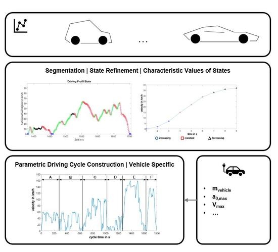
Starting point are the driving profiles of a heterogeneous data set. In the first step, the segmentation into the four global driving states acceleration, deceleration, oscillation and idling takes place. The data analysis in the second step comprises the state refinement and serves to derive characteristic values for each driving state. The results here are, on the one hand, the completely segmented driving profiles, as well as so-called relevant matrices that characterize a driving state. For each driving state S₁ to S₁₂, the relevant matrices contain the characteristic values required for the parametric calculation of a driving segment of the corresponding state. More details are shown below. In the third step, the transition matrix can be calculated with this, before a driving cycle is parametrically calculated in the final fourth step.

3.2.1. Used Database

The presented method is shown based on a real driving data record according to the framework shown by Wittmann et al. [15]. Here, an existing database is used, which has been entered with different vehicles, from small cars to luxury class, in different contexts. The journeys were recorded with the internal sensors of smartphones at a sample rate of 1 Hz. The recorded velocity profile is used for calculation of the acceleration profile by a Euler forward approach. All journeys were carried out in Germany, Switzerland and Italy. The consideration of journeys with maximum speeds above 200 km/h represents a first difference to current driving cycles. A heterogeneous data set with city, rural and highway trips is available, whereby in a recorded trip all or even one of these areas may be prominent. An exact subdivision into these areas cannot be made due to the lack of data. Therefore, the transferability of the method is given for all data sets. The majority of the vehicles use a conventional drive (ICEV). The reason for this is the use of mainly private vehicles to record journeys with a smartphone. There is a heterogeneous data set with city, rural and motorway trips, whereby in a recorded trip all or even only one of these areas may stand out. An exact subdivision into these areas cannot be made due to the lack of data knowledge. A total of 3950 km of journey data with a total time duration of 66 h is available.

3.2.2. Data Segmentation

For the EMCC methodology, a new two-stage segmentation approach is shown, which in the first stage prescribes concrete characteristic values for all global driving states. Initially, it is not required that a driving point can only be assigned to exactly one of the four global driving states acceleration, deceleration, oscillation and idling. Note that oscillation in a speed window is composed of acceleration and deceleration. The unambiguousness, which is absolutely necessary to derive the transition matrix, is achieved by the second segmentation stage in a logic.

Step 1: Pre-Segmentation

First, the criteria to be met for each driving condition are set. A driving sequence is identified as an acceleration sequence if for at least 3 s the acceleration in each individual driving point is greater than a_i ≥ 0.01 m/s² and the sum of the acceleration values in the driving points is greater than a_sum ≥ 0.1 m/s². A deceleration sequence is defined in an analogous manner. A travel sequence is a deceleration sequence if the acceleration is less than a_i ≤ −0.005 m/s² for at least 3 s and the sum of the acceleration values in the individual travel points is less than a_sum ≤ −0.1 m/s². Previous procedures define all points in a travel profile which have not been identified as acceleration or braking states as oscillating or idling states. Here, however, defined criteria are also to be set for these two driving states. To identify a cruising sequence, a driving sequence with a duration of 10 s is examined. The driving sequence is a cruising sequence if the deviation of the speed in the individual driving points from the average speed of the examined sequence does not exceed a defined tolerance window. This tolerance window is assumed as a function of the average speed of the examined sequence in order to avoid too strong a generalization. The permissible tolerance decreases with increasing speed. The tolerance range is between 25% at very low speeds to 2% at very high speeds. The identification of an idle state is only carried out on the basis of the driving speed. If the driving speed is lower than v_i ≤ 1 km/h for at least 3 s, an idle state is assumed for this sequence. The following figure shows a classified driving sequence according to the criteria mentioned above (Figure 9).

The figure shows that a cruising sequence is composed of acceleration and deceleration states. Therefore, driving points can be assigned to more than one global driving state.

Step 2: Unambiguousness

To decide whether a driving point belongs to an acceleration, deceleration or cruising sequence, a logic is used which is based on four principles.

• A cruising sequence is not interrupted by an acceleration sequence that is shorter than the current cruising sequence, e.g., in Figure 9. at time 1415 s.
• A cruising sequence is not interrupted by a braking sequence that is shorter than the current cruising sequence, e.g., in Figure 9. at time 1420 s.
• An acceleration sequence is not interrupted by a subsequent cruising sequence that is detected, e.g., in Figure 9. at time 1550 s.
• If the deceleration sequence is longer than the cruising sequence which has also been detected, the cruising sequence is interrupted at the starting point of the deceleration sequence. The braking sequence then dominates, e.g., in Figure 9. at time 1530 s.

The Figure 10 below shows the result after applying this logic.

This two-stage classification procedure enables the robust and unambiguous assignment of driving sequences to the four global driving states with fixed criteria. From the nearly 4000 km of driving data, 4410 acceleration, 4204 deceleration, 3368 cruising and 538 idling sequences can be extracted by the two-stage segmentation method. For the data set used, over 95% of all driving points can thus be assigned to one of the four global driving states. Non-assigned points have no influence on the results of cycle construction, as in the approach presented here no real driving segments are linked, but rather these are constructed parametrically.

3.2.3. Data Analysis

In order to avoid a generalization of the characteristic values of the individual states, the driving sequences are subdivided into different speed ranges analogous to [10]. For the set of driving sequences of a global driving state and speed range the evaluation and derivation of the characteristic values is done in three steps. In the first step a state refinement is applied to justify the assumption of a 1st order Markov chain. From the four global states, 12 driving states (S₁–S₁₂) are derived. Accordingly, after this step, a set of driving sequences is available for each driving state S₁–S₁₂.

For the parametric simulation of a sequence of these driving states, a set of characteristic values is required for each state. These differ from state to state and in general include the duration t_seq and initial acceleration a_start of the corresponding state. In the second step, therefore, these descriptive characteristic values are identified. Once the variables have been identified for each state, these characteristic values can be assigned in the third step by means of a statistical analysis.

Sequences of acceleration and deceleration:

The global acceleration and deceleration sequences are first divided into sub-states (Figure 8). The following Figure 11 shows a subdivided global acceleration and deceleration sequence in the corresponding sub-states.

The states of increasing acceleration (S₁) and increasing deceleration (S₄) are defined as follows:

$$\frac{{\mathrm{a}}_{\mathrm{i}+1}}{{\mathrm{a}}_{\mathrm{i}}}>1.17\mathrm{and}\frac{{\mathrm{a}}_{\mathrm{i}+2}}{{\mathrm{a}}_{\mathrm{i}+1}}>1.17$$

(4)

In most cases, one of these states can be detected at the beginning of an acceleration sequence or deceleration sequence. Depending on the total duration of the sequence to be segmented, a state of uniform acceleration usually follows, referred to below as state S₂ or S₅.

$${\mathrm{a}}_{\mathrm{i}+1}\approx {\mathrm{a}}_{\mathrm{i}}$$

(5)

This state can last from one to many seconds, depending on the duration of an acceleration or deceleration process. The end of a global acceleration or deceleration sequence is usually characterized by a flattening of the acceleration value. The following applies to states S₃ (acceleration) and S₆ (deceleration):

$$\frac{{\mathrm{a}}_{\mathrm{i}+1}}{{\mathrm{a}}_{\mathrm{i}}}<0.85\mathrm{and}\frac{{\mathrm{a}}_{\mathrm{i}+2}}{{\mathrm{a}}_{\mathrm{i}+1}}<0.85$$

(6)

For the choice of the conditions set in Equations (4) and (6) for state refinement, a compromise between robust state assignment and generalization must be chosen. For each state S₁–S₆, further characteristic values are derived from the set of corresponding sequences, which allow to construct such sequences parametrically. In the following, the further evaluation for the acceleration states S₁–S₃ is shown. The evaluation of the deceleration states follows the same procedure and is not shown further here.

The following

Table 1. Identified characteristic values.

S1	S2	S3
${\mathrm{t}}_{\mathrm{seq}}$	${\mathrm{t}}_{\mathrm{seq}}$	${\mathrm{t}}_{\mathrm{seq}}$
${\mathrm{a}}_{\mathrm{start}}$		${\mathrm{scale}}_{\mathrm{S}3}$
${\mathrm{scale}}_{\mathrm{S}1}$

shows the identified characteristic values which are necessary for the calculation of a driving segment of the corresponding state.

For the driving states S₁ and S₃, the acceleration in the next time step can be calculated using the scaling factor.

$${\mathrm{a}}_{\mathrm{i}+1}={\mathrm{a}}_{\mathrm{i}}{\mathrm{scale}}_{{\mathrm{S}}_{\mathrm{n}}}$$

(7)

For the driving state S₁ the acceleration value a_start is required for the first time step of this state. Since the state’s steady acceleration (S₂) and decreasing acceleration (S₃) usually follow on another acceleration state, the initial acceleration value is taken over from the last state in the first time step. After Equation (3) the driving profile can then be calculated for the duration t_seq.

After the state refinement and the identification of the characteristic values that are necessary for the parametric calculation of a driving sequence, the derivation of these values from the extracted real driving sequences is carried out in the third step of the data analysis. The following figure shows an example of the distribution for the sequence duration t_seq and the start acceleration a_start for a speed range of the driving state S₁ (Figure 12).

For each characteristic value of a driving condition and speed range it must be decided whether a constant value can be assumed or whether a frequency distribution must be taken into account. Furthermore, one of the identified characteristic values can depend on one of the other characteristic values. For the driving state S₁, the statistical evaluation has shown that a constant value can be assumed for the sequence duration t_seq. The start acceleration a_start is selected in accordance with a frequency distribution, for the scaling factor scale_S1 the value is determined as a function of the start acceleration. The characteristic values of a state are summarized in a matrix relevant for this state and velocity range (

Table 2. Characteristic values of a state.

Class	Relative Frequency	Initial Acceleration [m/s2]	Duration [s]	Scaling Factor
1	0.32228	0.04125	3.5411	2628
2	0.27624	0.10625	3.5411	1886
3	0.15891	0.18047	3.5411	1673
…	…	…	…	…

).

If the next state selected by the Markov chain is the driving state S₁ and the current cycle speed is within the range corresponding to this matrix, then the first row of this matrix is selected with a probability of 32.2%. For the further acceleration states S₂ and S₃, as well as the deceleration states S₄–S₆, an analogous data analysis is performed. In the following

Table 3. Identified characteristic values.

Driving State	Name	Number of Velocity Ranges	Characteristic Values
			Variable	Constant
S1	increasing acceleration	3	initial acceleration, scale (matched)	duration
S2	constant acceleration	3	duration	-
S3	decreasing acceleration	3	scale	duration
S4	increasing deceleration	3	initial deceleration, scale (matched)	duration
S5	constant deceleration	3	duration	-
S6	decreasing deceleration	3	scale	duration

, the identified characteristic values for these states are summarized again.

Sequences of Cruising:

For the acceleration and deceleration sequences, a subdivision into three speed ranges was applied [10]. For the evaluation of the cruising sequences, the EMCC methodology proposes a finer subdivision into five ranges. The limit values are 55, 80, 100, 130 km/h (Figure 13).

For each of these speed ranges, an evaluation is carried out according to the procedure described above. In their work, SCHWARZER and GHORBANI show a method that represents cruising sequences as speed noise. For the EMCC method a simplified modelling of a cruising sequence is to be applied. Such a sequence can be described and parametrically modelled by means of three characteristic values (Figure 14).

Besides the sequence duration t_seq the limits of the acceleration value a_{(limit,pos/neg)} are needed. For each point in time of the cruising state, an acceleration value is then randomly selected which lies within these limits. As a result, the driving speed varies in a small window around the initial speed, which corresponds to the definition of a cruising sequence on which this paper is based. This simplified approximation of cruising sequences is considered appropriate for the objective here. However, the method shown by SCHWARZER and GHORBANI certainly offers higher accuracy.

For the consideration of cruising sequences of different lengths, the definition of a global cruising state is not sufficient. Even for speeds up to 55 km/h the duration of the identified cruising sequences in the real data varies from one to more than 100 s. Therefore, a state refinement is also applied here. In each speed range, five cruising states S₇–S₁₁ are defined, which are characterized by a different cruising duration. The limit values for the duration of a state vary for each speed range, but are set in such a way that after the cruising sequences have been divided into these driving states S₇–S₁₁, a fixed prescribed frequency distribution results. For example, 45% of the extracted cruising sequences of a speed range belong to the driving state S₇. As a result of this state refinement, the range of the cruising duration t_seq of one state decreases significantly.

For each driving state S₇–S₁₁ and speed range the statistical evaluation and derivation of the above identified characteristic values t_seq, a_(limit,pos), a_(limit,neg) is carried out according to a uniform procedure. The duration t_seq of a cruising sequence is chosen quasi randomly according to the frequency distribution found in the real data (Figure 15).

The minimum and maximum acceleration a_{(limit,pos/neg)} is the average value of a class formed for the duration of a cruising sequence. The following table shows a section of the relevant matrix for the driving state S₇ (<55 km/h) (

Table 4. Relevant matrix for the driving condition S₇.

Class	Relative Frequency	Duration In s	Max. Acceleration in m/s2	Max. Deceleration in m/s2
1	0.092783505	1	0.001340254	−0.002380952
2	0.06921944	2	0.050723404	−0.034638298
3	0.082474227	3	0.030321429	−0.105107143
…	…	…	…	…

).

If the next state selected by the Markov chain is driving state S7 and the current cycle speed is below 55 km/h, then with a probability of 7% this state will last for 2 s and the acceleration values will be between −0.035 m/s² and +0.05 m/s² (class 2). Depending on the speed range and cruising state, these characteristics vary.

In summary, for each driving state S₁–S₁₁ and the different speed ranges such a matrix exists with all relevant characteristic values and the frequency distributions to be taken into account. With the help of this matrix, segments of the driving states can be calculated parametrically.

Sequences of Idle:

For the remaining idle state S₁₂, the duration of such a state is used as the only characteristic value. The speed and acceleration must be set to zero. In addition to traffic conditions, such as red lights or traffic jams, the duration of an idling sequence is also significantly influenced by the driver and his intentions. The data set used here was recorded with smartphones. Whether the vehicle was actually idling or whether the journey was simply not interrupted manually on the smartphone and the vehicle was already parked cannot be reconstructed from the data set. Therefore, the duration of an idle state will not be derived from the real driving data in this paper. The duration of the driving state S₁₂ is randomly chosen between one and 90 s. This value corresponds to the maximum circulation time of a traffic light and is considered useful here [15]. For the results in this paper, an equal distribution for values between 1 to 90 s is used. However, this can be adapted to specific applications, e.g., city cycles.

This means that the characteristic values required for the parametric calculation according to Equation (3) are known for all 12 driving states. The 12 driving states are linked to a driving cycle by a 1st order Markov chain.

3.2.4. Markov Chain and Transition Matrix

For the complete definition of a Markov chain, the so-called initial distribution is required in addition to the transition matrix P. This is defined for a Markov chain (X₀, X₁, ...) with the states (S₁, S₂, ..., S₁₂) by a row vector [10].

$${\mathsf{\mu }}^0=\left(\mathrm{P}\left({\mathrm{X}}_0={\mathrm{S}}_1\right),\dots ,\mathrm{P}\left({\mathrm{X}}_0={\mathrm{S}}_{12}\right)\right)$$

(8)

For the vehicle to start moving at the beginning of a driving cycle, the first driving state must be an acceleration state. The increasing acceleration state (S₁) is set as the first state. The state distribution for the time t = 0 s is thus obtained:

$${\mathsf{\mu }}^0={\mathrm{S}}^0=\left[100000000000\right]$$

(9)

In total, 12 generally valid driving states were defined and all real driving profiles were subdivided into these driving states. The EMCC method therefore allows the use of a single constant transition matrix P_ij. The entries of the transition matrix are calculated according to Equation (2). The following transition matrix results for the data set used here (Figure 16).

The transition matrix shows that the state refinement was justified and the underlying assumptions in Section 3.1 can be confirmed. For example, the state S₁ is followed with a probability of 99% by a further acceleration state S₂ or S₃.

Starting from the initial state distribution S⁰ the next state distribution is calculated by a 1st order Markov chain.

$${\mathrm{S}}^1={\mathrm{S}}^0{\mathrm{P}}_{\mathrm{ij}}=\left[\mathrm{0\; 0.80\; 0.19}\dots \right]$$

(10)

For further calculation, a unique state must be determined from this probability distribution. For this purpose, the common method of the weighted number generator is chosen [6]. With a probability of 80%, driving state S₁ is followed by driving state S₂. With the help of the characteristic values of the 12 driving states and the Markov chain recorded in the relevant matrices, the driving cycle can finally be calculated.

3.2.5. Calculation of Driving Cycle

According to Equation (3) the driving cycle can be calculated iteratively. If the state is determined by the Markov chain, the associated travel segment can be calculated using the characteristic values of this state. For this purpose, a state vector is defined which comprises all characteristic values of the selected travel state and the current cycle speed. For the first driving state S₁ of a driving cycle after the initial distribution, the following state vector results as an example.

$${\mathrm{state}\mathrm{vector}}_{\mathrm{t}=0}=\left[\begin{array}{c}{\mathrm{v}}_0\\ {\mathrm{t}}_{\mathrm{seq}}\\ {\mathrm{a}}_{\mathrm{start}}\\ {\mathrm{scale}}_{\mathrm{S}1}\end{array}\right]=\left[\begin{array}{c}0\mathrm{km}/\mathrm{h}\\ 4\mathrm{s}\\ 0.11\mathrm{m}/{\mathrm{s}}^2\\ 1.89\end{array}\right]$$

For this state vector, a driving segment with a duration of 4 s is calculated starting from an initial speed of zero according to the following relationship.

$${\mathrm{v}}_{\mathrm{i}}={\mathrm{v}}_{\mathrm{i}-1}+\left({\mathrm{a}}_{\mathrm{start}}{1.89}^{\mathrm{i}-1}\right)\left({\mathrm{t}}_{\mathrm{i}}-{\mathrm{t}}_{\mathrm{i}-1}\right)\mathrm{for}\mathrm{i}=1\dots 4$$

(11)

where t is the current cycle time. In this way, the corresponding travel segment can be calculated for each of the next selected travel states of the Markov chain. This is repeated until the desired cycle length is reached.

The EMCC methodology presented here builds up motion segments for the defined motion states based on the characteristic values. In contrast to the linking of real driving segments in the previous methods according to [6,7,9,13], the shown EMCC method requires that physically reasonable limit values be observed. The Markov chain has no knowledge that the driving state S₄ (increasing deceleration) cannot be assumed at the current cycle speed close to zero, since otherwise a speed below zero results due to negative acceleration.

The two major interventions to maintain the physical limits are achieved by setting a minimum speed of 0 km/h and a vehicle-specific maximum cycle speed.

The parametric cycle design presented here allows to generate a driving cycle specifically for one vehicle class based on one global data set. Whether a cycle is drivable for a vehicle depends not only on the already limited maximum speed but also on the acceleration ramps. A sports car will run operating points over its lifetime that a small car cannot reach. By limiting the maximum cycle acceleration, it is possible to react specifically to the vehicle class. Since the acceleration capacity depends on the current vehicle speed, the maximum possible acceleration is not assumed to be constant but is determined by a simplified longitudinal dynamics model based on the current cycle speed.

By means of the parametric cycle calculation shown and the targeted interventions in it, a specific driving cycle can be generated if vehicle-specific characteristic values are known. Exemplary results are presented in the following section.

4. Results and Validation

The underlying assumption of the EMCC methodology shown in this paper is the definition of a driving cycle in the form of a stochastic process. This is further modelled by a 1st order Markov chain. An elementary result is the non-deterministic behavior of the cycle construction. An infinite set of different driving cycles can be generated while maintaining the vehicle class specific characteristics. Different vehicle classes have to meet different requirements regarding the powertrain, so that representative driving cycles for each vehicle class represent a considerable gain in knowledge. The following

Table 5. Boundary conditions for the driving cycles.

Cycle Time in s	Change City Rural at Time in s	Change Rural Highway at Time in s	Min. Velociy in km/h	Max. Deceleration in m/s2	Max. Velocity/Acceleration
1800	600	1200	0.1	−3	vehicle specific

summarizes the set boundary conditions for the driving cycles discussed in this chapter.

The total length of a cycle here is based on the duration of the WLTC. The proportions of city, rural and motorway are equally distributed and are only simulated by setting the maximum cycle speed. However, it could be more precise if the proportion of city, rural and motorway is adopted to the considered vehicle class. For further comparison of different driving cycles this could be neglected. By specifying the maximum acceleration and top speed, as well as other vehicle characteristics, a driving cycle can be generated that requires operating points that are close to the performance limits of the powertrain. The following figure shows an exemplary driving cycle for the small car class and the luxury class (Figure 17).

According to the unlimited speed on German highways, for the small car cycle a maximum speed of v_(max,small) = 160 km/h and a maximum initial (v = 0 km/h) acceleration a_(0,small) = 2.0 m/s² is assumed here. Significantly higher values can be applied for the driving cycle of the luxury class. A maximum speed of v_(max,exe) = 250 km/h and a maximum initial acceleration of a_(0,exe) = 4.0 m/s² is permitted. The differences can also be easily seen in the generated cycles in (Figure 17).

Since the method presented in this thesis does not link real driving segments, the drivability of a driving cycle is not directly given. With previous methods of cycle design, the selection of a representative driving cycle is performed by comparing the speed-acceleration distribution of the cycle with the real driving data [5]. For a heterogeneous data set, driven by different vehicles in different traffic environments, such an approach is not possible for the methodology shown here. For a heterogeneous data set used here, a comparison of the SAFD is only possible if concrete data knowledge is available. The data set must then be classified according to vehicle classes. In this case, the common comparison of SAFD provides information about general representativeness of driving behavior [5]. Such data knowledge is not available for the data set used here. In order to be able to make a statement about the constructed driving cycles nevertheless, a categorization based on a characteristic value is first shown.

4.1. Valuation Based on a Characteristic Value

A Categorization Value (CV) is introduced, which reflects the stress on a vehicle caused by a driving cycle in comparison to other driving cycles. For the calculation of the CV, this thesis uses the following characteristics of a driving cycle, which can be directly related to the load of a vehicle by the driving cycle: the average speed with respect to the maximum vehicle speed v_(avg,%); the idling portion n_LL; the portion of acceleration states s_(acc,%); the portion of accelerations exceeding 70% of the maximum possible acceleration a_(max,70,%) and the portion of decelerations exceeding 70% of the maximum deceleration a_(min,70,%). To calculate the CV, 400 driving cycles for each vehicle class (same input parameters) were constructed using the approach shown here. For each characteristic C_cycle,i of a driving cycle, the minimum C_min,i, and maximum value C_max,i of the underlying 400 cycles are used to calculate the CV for the corresponding characteristic.

$${\mathrm{CV}}_{\mathrm{cycle},\mathrm{i}}=1+\frac{9}{{\mathrm{C}}_{\max ,\mathrm{i}}-{\mathrm{C}}_{\min ,\mathrm{i}}}\left({\mathrm{C}}_{\mathrm{cycle},\mathrm{i}}-{\mathrm{C}}_{\min ,\mathrm{i}}\right)$$

(12)

In order to be able to derive a rapid tendency of the vehicle load of a driving cycle, the global CV value is calculated, which transfers the five characteristic values CV_cycle.i weighted in equal proportions into a scale between 1 and 10, where CV = 10 indicates a high vehicle load. The average cycle speed is then over 50% of the maximum speed. The idling component is then close to zero. In addition, high accelerations and decelerations often occur. The driving cycle will also be highly dynamic, as over 45% of the driving conditions correspond to a state of acceleration. These conditions clearly indicate a high vehicle load. Nevertheless, it should be noted that the CV value is a relative valuation according to other driving cycles.

The Figure 18 below shows how driving cycles with different CV values differ.

Shown here are two driving cycles for the compact class with different CV values. For this vehicle class, the maximum vehicle speed v_{(max,compact)} = 210 km/h and a maximum initial acceleration a_max = 3.0 m/s² are assumed. The blue curve shows a driving cycle with a resulting CV value of CV = 5.9, the cycle shown in green has only a value of CV = 4.7. The difference can be seen on the one hand in the significantly increased dynamics in the urban area and on the other hand in the higher maximum and average cycle speed.

Whether a driving cycle is drivable for a vehicle in reality cannot be shown so far. Therefore, the validation of the methodology shown here includes a test on a chassis dynamometer.

4.2. Driveability Check

For the validation of the driving cycles a roller test bench with a rotating roller is used. The non-driven axle of the test vehicle is firmly clamped by the fixation of the tires [16] The test vehicle used here is a VW eGolf with front-wheel drive, whose maximum acceleration is $2.9\mathrm{m}/{\mathrm{s}}^2$ and maximum speed is 140 km/h [17]. The exact sequence of the speed specification by the driving cycle is controlled by a pedal robot, which actuates the accelerator and brake pedal of the vehicle. The aim of the driveability test is to check the set limit values of acceleration, as these are decisive for the driveability of the driving cycle by the vehicle. The driving cycle shown below (Figure 19) is a suitable cycle for this purpose.

It is easy to see that the actual course follows the target course well over long distances. The required acceleration process from the 300th second is implemented almost exactly by the test vehicle. For this acceleration section a maximum acceleration of 1.1 m/s² is called up by the driving cycle. The maximum possible acceleration calculated by a simplified longitudinal dynamics model is 1.7 m/s² at this point in time. For the acceleration process at second 470, here marked by a blue frame, the actual course shows that the test vehicle can hardly follow the target speed towards the end of the sequence. For this point in time, the driving cycle requires an acceleration of 1.7 m/s². This value corresponds exactly to the maximum possible acceleration predicted from the vehicle data and the current vehicle speed via the longitudinal dynamics model. Since the actual speed here shows a slightly flatter curve, the maximum possible vehicle acceleration is actually called up. This is also consistent with the observations of the speedometer during the driving cycle on the chassis dynamometer.

As a summary statement, it can be stated here that the predicted acceleration limit is maintained by the cycle design and this corresponds well with the real limit values of the test vehicle. By means of the Categorization Value the load capacity of a generated driving cycle can be estimated. A basic drivability was shown by a test on the chassis dynamometer. Finally, representative driving cycles are to be shown by way of example and compared with the WLTC.

4.3. Representative Driving Cycles for Powertrain Design

The aim of this paper is to generate driving cycles that can be used for the design and dimensioning of the powertrain. Therefore, driving cycles with increased dynamics and increased vehicle load are suitable for this purpose. In the following, a driving cycle for the small car class is shown as an example, which has a CV value of 7.8 and therefore causes a high load on the powertrain (Figure 20).

A maximum acceleration of a_max = 2.0 m/s² in the initial state and a maximum speed of v_max = 160 km/h is assumed for this vehicle class. After subdividing the driving cycle into sections A–F, each of these sections may be associated with a traffic condition. Sections A and B are generally assigned to urban traffic, where section A can be described as “light urban traffic”. The increased acceleration and braking usually occurs in “increased urban traffic” (Section B). Section C is referred to here as “dynamic interurban travel”. This section is characterized by frequent acceleration and braking. Section D is a general “stop and go” segment. This can occur both in city traffic and when driving on the motorway. The concluding sections E and F form two motorway sections. For section E, the maximum speed is reached, this section is associated with a “free motorway journey”. For the following section F, the cycle speed is limited to the recommended speed. Therefore, this section can be described as “restricted motorway travel”. In addition to these assigned areas, the cycle is characterized by the following characteristics. Overall, 43% of the times of this driving cycle are acceleration states, 6% of which have an acceleration that is at least 70% of the maximum possible acceleration. In total, 11% of the points in time are driven at a speed that is at least 80% of the maximum vehicle speed. If 99% of the maximum speed is reached, the same applies to the limit of maximum acceleration. This reaches 98%. These characteristic values result in an average speed of v_(avg,%) = 0.34 (34% of the maximum speed) and in an idling ratio of 2%. These characteristic values result in the high CV for this driving cycle.

Taking into account the maximum speed v_(max,WLTP) = 131.7 km/h and the maximum acceleration a_(max,WLTP) = 1.75 m/s², it can generally be said that the WLTC is not well suited for the design and dimensioning of the powertrain. Even for the small car class, these limits are well below the possible accelerations and speeds of a typical vehicle in this class. The figure below shows a direct comparison of the WLTP with the driving cycle recommended in this paper for the small car class (Figure 21).

If one calculates the CV value resulting from the WLTC for the small car class, one gets CV = 3.2, which once again shows that the WLTC is not a relevant load. With increasing vehicle class, the relevance decreases further. The final figures show a direct comparison of the WLTC with the driving cycles proposed here as examples for the compact class and the luxury class (Figure 22).

Finally, it should be noted that the cycles shown are suggested for the design of the drive train. If the general average driving behavior is to be mapped, for example to determine fuel consumption, cycles with lower CV values are recommended.

5. Conclusions

Current driving cycles, such as the WLTC, are suitable for comparing different vehicles, as they provide reproducible results under laboratory conditions. However, they generally do not represent real driving behavior and, moreover, they do not apply across vehicle classes. Therefore, current regulatory driving cycles are not appropriate for optimal performance design of the powertrain, with respect to maximum acceleration and high-load operations.

Current methods for designing driving cycles using real driving data were shown and their suitability for the design of vehicle classes of specific driving cycles was discussed. The methods shown fulfil the criteria in some points, but none of them could be used for the intended purpose. Therefore, a new method for parametric cycle construction was shown, which is based on the state-based method of LIN and NIEMEIER [6] and is therefore called Enhanced Modal Cycle Construction (EMCC). This methodology enables a fully parametric cycle construction by state refinement. The global driving states acceleration, deceleration, cruising are further divided into sub-states. This step enables the construction of a complete driving cycle through a single 1st order Markov chain with a constant transition matrix. The driving segments to be linked are calculated parametrically using characteristic values. The characteristic values could be obtained from the real driving data by statistical analysis. This makes it possible to force high accelerations in a targeted manner, which can occur more frequently in Battery Electric Vehicles (BEV) in particular, and are therefore absolutely necessary for the design.

By targeted interventions in the cycle design, it is possible to design specific driving cycles for specific vehicle classes, which cause a significant load on the drive train and can thus be used for the powertrain design and dimensioning. Validation on a roller test bench has shown that the drivability of the driving cycles is guaranteed when taking into account the vehicle-specific limit values, and thus the reality is well represented. Driving cycles can be compared with each other via an introduced Categorization Value. The value also allows conclusions to be drawn about the load of the driving cycle on the powertrain.

The validation of the generated driving cycles still represents an uncertainty. In future work, the cycles shown here should be checked with the help of vehicle class specific data sets. Furthermore, a comparison with driving data from BEV should be investigated to show to what extent the transferability of ICEV driving data to driving behavior in BEV can be guaranteed. Another future application of the method shown here is the representation of different driving styles for autonomous vehicles, which can be represented by changing acceleration rates and top speeds [18].

References

1. Zhou, W.; Xu, K.; Yang, Y.; Lu, J. Driving Cycle Development for Electric Vehicle Application using Principal Component Analysis and K-means Cluster: With the Case of Shenyang, China. Energy Procedia 2017, 105, 2831–2836. [Google Scholar] [CrossRef]
2. Volkswagen, A.G. Umstellung von NEFZ auf WLTP. Available online: https://www.volkswagenag.com/de/group/fleet-customer/WLTP.html (accessed on 3 February 2020).
3. Deutscher Bundestag, Finanzauschuss. Wortprotokoll der 103. Sitzung: Entwurf eines Gesetzes zur Änderung des Kraftfahrzeugsteuergesetzes. 2017. [Google Scholar]
4. Hofacker, A.; Christiane, K. WLTP und NEFZ im Vergleich. Available online: https://www.springerprofessional.de/fahrzeugtechnik/emissionen/wltp-und-nefz-im-vergleich/6560846 (accessed on 3 February 2020).
5. Gewald, T.; Reiter, C.; Lin, X.; Baumann, M.; Krahl, T.; Hahn, A.; Lienkamp, M. Characterization nd Concept Validation of Lithium-Ion Batteries in Automotive Applications by Load Spectrum Analysis. In Proceedings of the 31st International Electric Vehicles Symposium & Exhibition (EVS 31) & International Electric Vehicle Technology Conference (EVTeC), Kobe, Japan, 30 September–3 October 2018. [Google Scholar]
6. Lin, J.; Niemeier, D.A. Estimating Regional Air Quality Vehicle Emission Inventories: Constructing Robust Driving Cycles. Transp. Sci. 2003, 37, 330–346. [Google Scholar] [CrossRef] [Green Version]
7. Austin, T.C.; DiGenova, F.J.; Carlson, T.R.; Joy, R.W.; Gianlini, K.A.; Lee, J.M. Characterization of Driving Patterns and Emissions from Light-Duty Vehicles in California; Final Report; Sierra Research Inc: Street Sacramento, CA, USA, 1993. [Google Scholar]
8. Galgamuwa, U.; Perera, L.; Bandara, S. Developing a General Methodology for Driving Cycle Construction: Comparison of Various Established Driving Cycles in the World to Propose a General Approach. JTTs 2015, 5, 191–203. [Google Scholar] [CrossRef] [Green Version]
9. Dai, Z.; Niemeier, D.; Eisinger, D. Driving Cycles: A New Cycle-Building Method That Better Reprensents Real-World Emission. Ph.D. Thesis, UC Davis, Davis, CA, USA, 2008. [Google Scholar]
10. André, M. The ARTEMIS European driving cycles for measuring car pollutant emissions. Sci. Total Environ. 2004, 334–335, 73–84. [Google Scholar] [CrossRef] [PubMed]
11. Waldmann, K.-H.; Helm, W. Simulation Stochastischer Systeme: Eine Anwendungsorientierte Einführung; Springer: Berlin/Heidelberg, Germany, 2016. [Google Scholar]
12. Webel, K.; Wied, D. Stochastische Prozesse: Eine Einführung für Statistiker und Datenwissenschaftler, 2nd ed.; Springer: Wiesbaden, Germany, 2016. [Google Scholar]
13. Schwarzer, V.; Ghorbani, R. Drive Cycle Generation for Design Optimization of Electric Vehicles. IEEE Trans. Veh. Technol. 2013, 62, 89–97. [Google Scholar] [CrossRef]
14. Fries, M.; Baum, A.; Wittmann, M.; Lienkamp, M. Derivation of a real-life driving cycle from fleet testing data with the Markov-Chain-Monte-Carlo Method. In Proceedings of the 21st International Conference on Intelligent Transportation Systems (ITSC), Maui, HI, USA, 4–7 November 2018; pp. 2550–2555. [Google Scholar]
15. Wittmann, M.; Lohrer, J.; Betzet, J.; Jäger, B.; Kugler, M.; Klöppel, M.; Waclaw, A.; Hann, M.; Lienkamp, M. A holistic framework for acquisition, processing and evaluation of vehicle fleet test data. In Proceedings of the IEEE 20th International Conference on Intelligent Transportation Systems (ITSC), Yokohama, Japan, 16–19 October 2017; pp. 1–7. [Google Scholar]
16. für Straßen, FGSV–Forschungsgesellschaft. und Verkehrswesen (2010) Richtlinien für Lichtsignalanlagen (RiLSA). 2010. [Google Scholar]
17. Auto Motor und Sport. VW Golf Typ 5G Technische Daten zu allen Motorisierungen—Auto Motor und Sport. Available online: https://www.auto-motor-und-sport.de/marken-modelle/vw/golf/vii-typ-5g/technische-daten/ (accessed on 3 February 2020).
18. Schockenhoff, F.; Nehse, H.; Lienkamp, M. Maneuver-Based Objectification of User Comfort Affecting Aspects of Driving Style of Autonomous Vehicle Concepts. Appl. Sci. 2020, 10, 3946. [Google Scholar] [CrossRef]
Figure 1. Modelling a driving cycle with a Markov chain [6].
Wevj 11 00052 g001
Figure 2. Example of trip segmentation result by [9].
Wevj 11 00052 g002
Figure 3. Modelling of a driving pulse [13].
Wevj 11 00052 g003
Figure 4. Assessment of current methods for driving cycle construction.
Wevj 11 00052 g004
Figure 5. Exemplary state assignment to a driving sequence.
Wevj 11 00052 g005
Figure 6. Microscopic differences in acceleration sequences.
Wevj 11 00052 g006
Figure 7. Sub-states for one global acceleration sequence.
Wevj 11 00052 g007
Figure 8. Steps of driving cycle construction.
Wevj 11 00052 g008
Figure 9. Pre-Segmentation of a driving profile.
Wevj 11 00052 g009
Figure 10. Unambiguous segmentation of a driving profile.
Wevj 11 00052 g010
Figure 11. Subdivided states of acceleration and deceleration in real driving data.
Wevj 11 00052 g011
Figure 12. Frequency distribution of duration and initial acceleration for speed < 65 km/h.
Wevj 11 00052 g012
Figure 13. Division of cruising sequences in speed ranges.
Wevj 11 00052 g013
Figure 14. Characteristics of cruising sequences.
Wevj 11 00052 g014
Figure 15. Frequency distribution state S7 under 55 km/h.
Wevj 11 00052 g015
Figure 16. Transition matrix for used data set.
Wevj 11 00052 g016
Figure 17. Compressed driving cycle for small car and luxury class.
Wevj 11 00052 g017
Figure 18. Compressed driving cycles with different CV values for compact class.
Wevj 11 00052 g018
Figure 19. Used driving cycle for valuation on dynamometer.
Wevj 11 00052 g019
Figure 20. Suggested driving cycle and SAFD for powertrain design in small cars.
Wevj 11 00052 g020
Figure 21. Comparison of suggested driving cycle to WLTP.
Wevj 11 00052 g021
Figure 22. Suggested driving cycles for compact and luxury class.
Wevj 11 00052 g022