Cluster-Based Data Aggregation in Flying Sensor Networks Enabled Internet of Things

Abstract

Multiple unmanned aerial vehicles (UAVs) are organized into clusters in a flying sensor network (FSNet) to achieve scalability and prolong the network lifetime. There are a variety of optimization schemes that can be adapted to determine the cluster head (CH) and to form stable and balanced clusters. Similarly, in FSNet, duplicated data may be transmitted to the CHs when multiple UAVs monitor activities in the vicinity where an event of interest occurs. The communication of duplicate data may consume more energy and bandwidth than computation for data aggregation. This paper proposes a honey-bee algorithm (HBA) to select the optimal CH set and form stable and balanced clusters. The modified HBA determines CHs based on the residual energy, UAV degree, and relative mobility. To transmit data, the UAV joins the nearest CH. The re-affiliation rate decreases with the proposed stable clustering procedure. Once the cluster is formed, ordinary UAVs transmit data to their UAVs-CH. An aggregation method based on dynamic programming is proposed to save energy consumption and bandwidth. The data aggregation procedure is applied at the cluster level to minimize communication and save bandwidth and energy. Simulation experiments validated the proposed scheme. The simulation results are compared with recent cluster-based data aggregation schemes. The results show that our proposed scheme outperforms state-of-the-art cluster-based data aggregation schemes in FSNet.

1. Introduction

A multi-unmanned aerial vehicle (UAV)-aided flying sensor network (FSNet) is constrained by various energy factors, such as limited energy, computation, memory, and communication [1,2]. The energy consumption for sensing and computation is less than the energy used for communication among the UAVs or to the ground station (GS) [3,4]. The available energy resources are sometimes insufficient for transmission and computation during the mission. However, the collected data need to be communicated to the destination for further processing. The performance of the network lifetime depends on efficient energy utilization [5]. The researchers tried to minimize energy utilization in other wireless networks, but energy utilization still exists. Due to the flying speed of UAVs, the rapid variation in topology, terrain structure, and diverse directions make it difficult to collect and route information [6]. The researchers proposed energy-efficient schemes by considering different parameters such as reducing the communication distance, computation cost, mobility, and degree. However, data collection and minimization of communication load go unnoticed to save bandwidth and energy [7,8].

A data aggregation approach reduces the energy consumption of UAVs and increases their lifespan. The data aggregation approach is different in wireless sensor networks (WSNs) and vehicular ad hoc networks (VANETs) from UAV networks [9]. In WSN, the uses of the data aggregation approach are for decreasing energy consumption rather than minimizing network capacity usage [10]. In VANET, due to the high variation in the topology, data aggregation is performed by many vehicles. In addition to the degree, mobility, density, and other parameters, the multi-UAV system is constrained by energy factors, which is why it is compatible with WSN and VANET requirements [11]. UAVs also consume energy by processing and storing more data, just like flight and communication [12].

UAV-based data aggregation has emerged as a promising solution for collecting data from remote and hard-to-reach areas. One of the main motivations for UAV-based data aggregation is the ability to obtain data more efficiently and accurately. UAVs can cover a larger area in a shorter amount of time compared to traditional data collection methods. This means that data can be collected faster, allowing for a quicker analysis and quicker decision-making. Additionally, UAV-based data aggregation can also reduce data collection costs. Traditional methods often require expensive equipment and personnel, whereas UAVs can be operated by a single person and require minimal equipment.

The fundamental operation in FSNet is data aggregation, which aims to transmit data among UAVs or to the GS. The data aggregation approach reduces communication costs and bandwidth utilization while obtaining aggregated data. Data aggregation utilizes the concept of many-to-few. A data aggregation protocol describes how the data are gathered, how they are routed to the destination, and when they should be transmitted.

Therefore, in this study, we developed a cluster-based data aggregation scheme for UAV-based FSNet. This research contributes the following:

• An effective mechanism designed based on a honey-bee algorithm (HBA) to select optimal unmanned aerial vehicles–cluster head (UAVs-CH).
• The formation of balanced and stable clusters reduces re-affiliation rates.
• Data aggregation algorithm proposed to limit duplicated data communication to the base station (BS).
• Avoids the transmission of unwanted packets to the BS and save FSNet bandwidth.
• Mathematical techniques measure the accuracy and correctness of the proposed scheme.

The remaining article is structured as follows: Section 2 elaborates on the existing literature. Section 3 discusses the proposed cluster formation and data aggregation schemes. In Section 4, experiment evaluation and simulation outcomes are outlined. In the Section 6, the paper concludes and states future directions.

2. Background

This section reviews the existing work on energy-efficient clustering and UAV-based data aggregation approaches. A UAV-based data aggregation network architecture differs significantly from a traditional wireless sensor network. For these reasons, existing algorithms for stationary or low-mobility WSNs are not feasible [13]. A data aggregation algorithm based on UAVs needs to be able to adapt to networks with high mobility, sudden changes in topology, and sporadic communication links. WSNs require different levels of quality of service, including delay, packet loss, and reliability on the underlying networks. Furthermore, WSNs are limited in terms of energy, computation power, and network resources. An appropriate data aggregation technique is essential for meeting requirements while respecting WSN limitations. WSNs require time synchronization to coordinate data, energy, and localization. To address the sensor time synchronization problem, the authors of [14] proposed a pairwise broadcast synchronization (PBS) protocol for multi-cluster sensor networks that reduces overall energy consumption while maintaining synchronization accuracy. Reference [15] proposed a distributed heuristic algorithm for selecting appropriate sensors in a multi-hop sensor network to reduce the number of message exchanges needed for network-wide synchronization using PBS.

2.1. Energy Efficient Clustering

Energy-efficient clustering strategies for FSNet are still in their infancy [16]. This section presents an overview of some existing energy-efficient solutions based on different parameters, criteria, and approaches. FSNet has many military and civil applications. Nevertheless, the main issues of UAVs in FSNet are limited energy, high mobility, frequent topology changes, and terrain structure, due to the limited flight time of UAVs and lack of routing efficiency [17]. Aadil et al. [18] addressed these issues and proposed a clustering model with energy-aware link-based clustering called EALC. For efficient clustering, parameters such as energy, degree, cluster formation, and cluster head lifetime are taken into account. Link quality and transmission range are considered first to reduce the energy consumption of flying nodes. The K-means density-clustering model used for high mobility considers distance and energy. This model selects cluster heads (CHs) with the least computation and maximum throughput and minimizes routing overhead. The lifetime of UAVs increased with the use of an energy-efficient selection of CHs. A simple clustering approach is used to reduce computation overhead. Nevertheless, EALC ignored the communication load, data aggregation, and bandwidth utilization factors.

Arafat and Moh [19] proposed an energy-efficient clustering scheme based on particle swarm optimization for an emergency mission. First, implement swarm-intelligence-based localization and clustering (SIL and SIC) schemes that define the search space with a boundary box to reduce computation power. UAVs are placed randomly in the search space. SIL uses a grouping scheme to calculate the distance between the target UAVs. The proposed model has an estimation model to measure UAV distance from CH. The distance between nodes and CH is considered for reducing energy consumption. The Euclidean distance is utilized for locating UAVs and balancing cluster size. In SIC, cluster formation and CH selection are performed with a fitness function that considers remaining energy and distance. The performance metrics used in this paper are energy consumption, communication load, and delay. Node degree and residual energy are considered to balance inter-cluster and intra-cluster energy utilization.

Yang et al. [20] proposed a probabilistic energy-aware clustering scheme to find the most efficient path for UAVs using ant colony optimization (ACO). WSN data-gathering efficiency is achieved with UAVs. The network is divided into clusters, each with a CH, cluster members (CMs), and UAV. The nodes are stationary with a position-aware CH; the CH receives information from the UAVs flying around the cluster heads. The proposed model has three stages. First, a UAV senses data about the farmland event via the ground segment. Second, the data gathered by UAVs is transmitted to the data center through the CH. Finally, the data center contains a database and management information system.

To overcome packet loss, long delay, and increased routing overhead, Yu et al. [21] proposed a clustering protocol based on ACO to enhance network performance. A reliable link supervision method was established due to UAV mobility and topology variation. The nonlinear processing scheme increases buffer size and link load to control and avoid congestion on the link. Based on the density of UAVs, two routing strategies are proposed, namely sparse formation and concentrated formation. ACO-based polymorphism-aware routing integrates dynamic source routing and ACO.

2.2. UAVs-Based Data Aggregation

In FSNets, the collection and transmission of information through multiple hops increase energy utilization [22]. The data aggregation approach reduces energy utilization and increases network lifetime by minimizing UAVs load. The data aggregation approaches reduce the communication cost and energy consumption [23]. The researchers developed aggregation approaches for FSNet without redundant data elimination [24].

Wang et al. [25] introduced a UAV-assisted topology-aware data aggregation protocol in WSN (TA-UAV-DA). The data aggregation approach was inspired by the compressive sensing approach to reduce the errors rate in the data reconstruction process, extra overhead, and energy consumption. Balanced tree-based topology construction is performed to minimize the scope and update the matrix measurement. The CMs send data to CH, and UAV gathers data from the CHs. The simulation results show that the approach performs better when reconstructing data, and it is more efficient in data aggregation and storage constraints than a random walk and intelligent compressive sensing.

Wu et al. [26] developed an energy-efficient UAV-based data aggregation protocol (EE-UAV-DA) for WSNs. In EE-UAV-DA scheme, UAVs gather data as data mules. The proposed method calculates the optimum link for the data mule through all CHs, using a genetic algorithm that achieves high-energy efficiency. By balancing system throughput, the proposed approach reduces the delay between the sensors and the sink node. The optimization scheme provided by heuristic search identifies optimal solutions for joint CH selection and optimal routes for the data mule to decrease energy consumption. The objective function calculates and measures each solution’s quality for the optimum path.

Thammawichai [27] proposed optimizing communication and computation for multi-UAV information-gathering applications called OC-mUAV. Multi-hop clustering incorporates data aggregation by using a mixed-integer optimization formulation with mixed-integer nonlinear programming. In order to determine the roles of UAVs, the optimal control problem was formulated. The system framework tries to ensure that the optimal number of UAVs communicate with BS. To maintain minimum energy consumption during routing, each UAV acts as an aggregator. An adaptive energy consumption model minimizes energy consumption by considering sensing energy, aggregation energy, transmitting energy, and receiving multi-UAV energy. To reduce communication and communication energy, area mapping and target tracking were addressed during testing. Target and sensor models are used to select the sensor UAV based on a subset of UAVs. The distance between UAVs is used for mapping. As a result of the data aggregation framework, the network is flexible and reliable since it is a self-organized network, which prolongs the lifetime of the network due to multi-hop networks and provides better performance due to clustering of heterogeneous UAVs.

Dong et al. [28] proposed an algorithm to collect and process data in WSN, using UAVs and mobile agents (MAs) to search for victims at disaster sites. MAs move around the area to collect data from sensor nodes and share information with UAVs. The UAV assigns MAs to group leaders. The density of sensor nodes in a group known by the group leader has high residual energy and is an optimum link to a UAV. MAs’ routing is based on information-driven static and dynamic mobile agent planning algorithms. The proposed scheme is efficient in energy and time for any dense network using MAs and UAVs.

To decrease energy utilization in a UAV-aided WSN, Liu and Zhu [29] proposed an energy-efficient data collection method. Sensor nodes are placed randomly in the environment. The proposed approach uses three transmission modes to solve the short buffer size of sensor nodes to transmit data within the allotted time slots. The sensor node selects the modes, i.e., waiting, transmission to a sink node, and uploading to UAV in each discrete time slot. The sensor node is selected in waiting mode to sleep and not transmit the status of the node. The sensor node uploads data to the sink node in the second mode. In the third mode, the sensor node delivers data to the UAV based on the threshold value and distance condition during the UAV preplanned trajectory visit. The UAV of a fixed-wing aircraft is deployed at a constant velocity. This article uses a finite-horizon sequential Markov process and dynamic programming algorithm for the optimized transmission policy. Secondly, the proposed method optimizes the preplanned trajectory for UAVs using a recursive random search algorithm.

The authors of [30] analyzed the performance of an energy-constrained Internet of Things (IoT) system that uses a power beacon and UAV for data collection. The study examined how different system and channel parameters affect outage probability, outage capacity, and ergodic capacity. In [31], the authors explored the challenges and possible solutions for implementing a fully immersive and interactive industrial metaverse, which is a virtual space that interacts with the physical world in real time. In the paper, the authors focused on improving key performance indicators, such as the Age of Information, latency, and reliability through optimizing short-packet structures in 6G URLLC communication. A cooperative strategy involving an unmanned ground vehicle and UAV is proposed in [32] to collect data from sensor nodes (SNs) in UAV-enabled data collection systems when SNs may not be able to upload their data because of factors such as insufficient energy and low flight altitude. A collaborative strategy selection algorithm that combines multistage-based SN association and UAV-UGV path optimization algorithms was used to determine trajectories for mobile data collection nodes on the ground and in the air to minimize mission completion time.

3. Flying Sensor Network Cluster Optimization

In cluster-based flying networks, the selection of CHs and cluster formation requires special attention to decrease the re-affiliation rate and save FSNet resources [33]. To select CHs, essential parameters such as the remaining energy, mobility, and flying nodes degree are considered to obtain optimal clusters [34,35,36]. These parameters are optimized to distribute load among clusters. We use the clustering approach to balance and select CHs in accordance with [37], as shown in Figure 1. Data aggregation is initiated once clusters are formed.

As shown in Figure 1, the proposed approach begins with the selection of a CH-UAV. The selection process determines which UAV will act as the CH. If the node is the CH, it proceeds to the next step. Then, the CH-UAV broadcasts the time division multiple access (TDMA) schedules to all member nodes within its cluster. TDMA is a channel access method that allows multiple nodes to share the same communication channel by dividing it into different time slots. The CH-UAV receives data from all neighboring nodes within its cluster. Data aggregation is the process of combining or summarizing data from multiple sources. The CH-UAV performs data aggregation on the received data, reducing redundancy and improving efficiency. After data aggregation, the CH-UAV sends the aggregated data to the BS for further processing. If the current node is not CH, it proceeds to the next step. The non-CH node waits for the TDMA schedule broadcast by the CH-UAV. This schedule determines when the node can transmit or receive data. The algorithm checks the energy level of nodes. If the energy is still available, it returns to the CH selection step, indicating that the next round of the process will begin. When the node’s energy reaches zero or depletes, the flowchart terminates, and the process ends.

In cluster-based routing for flying sensor networks, CHs may receive multiple copies of the same dataset from different sensors located in the vicinity. The communication of data requires more resources as compared to computation. Hence, a method is required to discard duplicated packets when sending data to the base station at the cluster level. Thus, network resources such as batteries and bandwidth can be utilized for other purposes. The network lifetime will increase. Our proposed algorithm works in two phases: cluster setup and data aggregation.

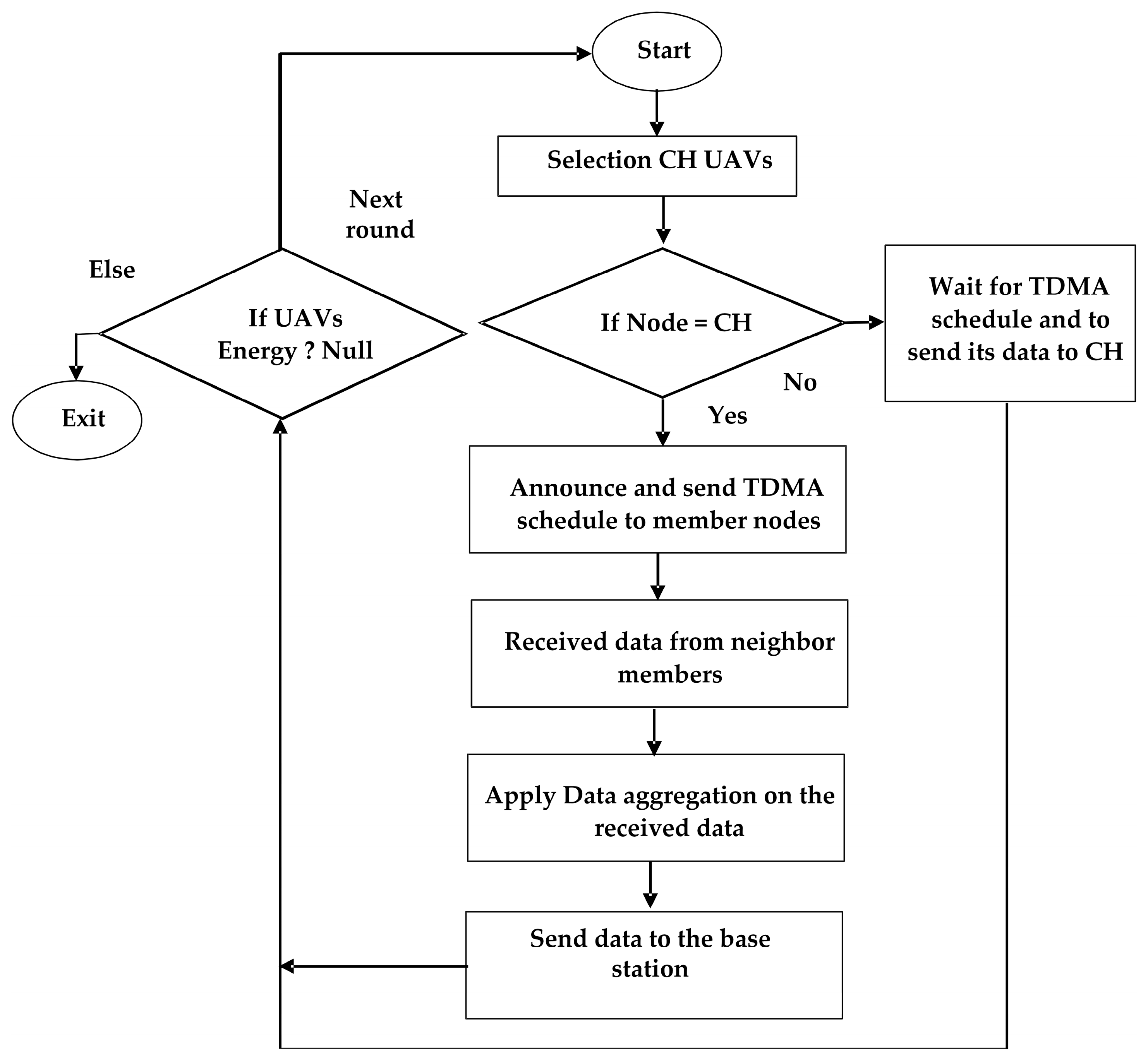
Clustering Setup

The HBA is applied in the cluster setup phase to determine the optimal CHs [37]. The CH selection is based on the HBA to form a balanced cluster. When selecting CHs, the UAV mobility and neighbor criteria are considered to minimize re-clustering. In FSNet, once CHs are selected, they broadcast a message containing ID, position, and status. All UAVs in CH range will receive broadcast messages and join the cluster. Once UAVs join a cluster, they become CMs and share information with CH. If a UAV receives membership messages from multiple CH, joining will be based on the distance between the UAV and CH. If the distance is the same, the random UAVS-CH selection mechanism will take place. The working of the cluster setup phase is shown in Algorithm 1 below. Once the cluster is formed, the data-aggregation-and-communication phase is initiated to transmit the data to the BS.

Algorithm 1: Pseudo Code of UAVs Enabled CH Selection.
1	Procedure CH-Selection-Multi-UAVs (MUAVs)()
2	$\mathrm{Input}: \mathrm{Swarm} \mathrm{of} \mathrm{UAVs} S{W}_{UAV}$$, \mathrm{UAV} \mathrm{nectar} [n_{UAV}$$], \mathrm{and} \mathrm{cluster} C_{FSNet}$.
3	Output: UAVs-CH
4	call function calculate-UAVs-Nectar ($n_{UAV}$) // v1 represents the number of nodes (UAVs) when there are n total UAVs in the network
5	$\mathrm{f}\mathrm{o}\mathrm{r}\left(v=1;v\le C_{\mathit{FSNet}};v++\right)$ do // selection of UAVs-CH in a random way
6	$\text{UAVs-CH}\left[\mathrm{v}\right]=\mathrm{functionRand} (S{W}_{UAV}$)
7	end for
8	while (highest-value! = yes) do
9	$\mathrm{f}\mathrm{o}\mathrm{r}\left(v1=1;v1\le n_{\mathit{UAV}};v1=v1+1\right)$ do // the suitability of current selection is computed
10	if (v1 in UAVs-CH) then
11	$\mathrm{Fitness} \mathrm{Value} FValu{e}_{UAV}=FValu{e}_{UAV}+1\left(S{W}_{UAV}\right[u]+AF{V}_{UAV})$ $// \mathrm{Average} \mathrm{fitness} \mathrm{value} AF{V}_{UAV}$
12	end if
13	end for
14	$\mathrm{if} (FValu{e}_{UAV}<PFValu{e}_{UAV}$) then $//PFValu{e}_{UAV}$ is the suitable value in the existing solution
15	$\mathrm{swap} FValu{e}_{UAV}$
16	end if
17	if (UAVs-CH-optimum! = yes) then
18	$\mathrm{w}\mathrm{h}\mathrm{i}\mathrm{l}\mathrm{e}(\mathrm{e}\mathrm{m}\mathrm{p}\mathrm{b}!=0)$ do   // Employed bee (empb) $// \mathrm{visiting} \mathrm{of} \mathrm{bees} \mathrm{employed} \mathrm{till} \mathrm{empty}, \mathrm{where} {\alpha }_{ij}$ is UAV affiliation with the current round while y is the neighborhood size
19	$UA{V}_j(x+1)=UA{V}_j\left(x\right)+{\alpha }_{ij}\ast y$ // selection of different UAVs from fellow citizen
20	end while
21	${\mathit{Pr}}_i=\frac{W_{UA{V}_i}}{{\sum }_{j=1}^k{W}_{UA{V}_j}}$ //$\mathrm{the} \mathrm{new} \mathrm{UAVs} \mathrm{probability} {Pr}_i$$\mathrm{will} \mathrm{be} \mathrm{calculated} \mathrm{based} \mathrm{on} \mathrm{Weight} \mathrm{of} \mathrm{UAV} (W_{UAV}$)
22	while (the Obees ≠ Є) do  //Onlooker bees (Obees)
23	$\mathrm{Selection} \mathrm{of} \mathrm{another} \mathrm{set} \mathrm{of} \text{UAVs-CH} \mathrm{will} \mathrm{be} \mathrm{carried} \mathrm{out} \mathrm{subject} \mathrm{to} \mathrm{the} \mathrm{probability} {Pr}_i$
24	end while
25	Else
26	return UAVs-CH
27	end while
28	end procedure

4. Data Aggregation and Communication

We collect data from flying UAVs and match the data to discard similar data sent by multiple sensors in the data aggregation process. Data aggregation is divided into two levels. In level 1, the data are collected using a TDMA schedule when multiple sensors simultaneously communicate data.

A near-linear time algorithm is proposed in this paper for the data aggregation level 2 problem in FSNet. The data coming from sensors is converted into a long string. According to our knowledge, this is the leading work to assume nontrivial alignment among the strings and the patterns. Specifically, we demonstrate the data aggregation problem in two ways: First, to sanction approximating $D\left[i\right]$’s, and second, an additional procedure sanction named partial data move, for the movement of partial data from one position to another in a data.

This similarity among the $X$ and $Y$ data is known as data match with moves (DMM) and designated as $d(X,Y)$ [38]. DMM is a powerful data-matching tool that can greatly benefit FSNet data aggregation. By using DMM, network operators can easily match data from different sources, allowing for a more accurate and comprehensive analysis of the data. The DMM algorithm can take advantage of UAV mobility by assigning them to different regions and optimizing their movement patterns to efficiently collect data. Moreover, DMM can provide a wide range of benefits, including reducing the amount of data, reducing bandwidth usage, increasing energy efficiency, and supporting proximity-based data aggregation. There are various applications in computational biology where partial data matches are considered a primeval in multiple situations. Moving a larger subsequence is similar to the insert or delete operation; during text processing, moving a large array together might be assumed, like reordering to deleting or inserting typescripts. Keep in mind that the nontrivial placements are still a challenge for DMM. Hence, $d(X,Y)$ is the size of the small structure of edit procedures that convert $Y$ to $X$; the allowable procedure affects the data stated. The deletion of a character at location, $loc$, transforms $X$ to $X\left[1\right]\dots X[loc-1],X[loc+1]\dots X\left[n\right]$.

• The insertion of a character, $“c”$ at a location, $“loc”$, gives $X\left[1\right]\dots X[loc-1],c,X\left[loc\right]\dots X\left[n\right]$.
• The substitution of a character at the location, $“loc”$, with character, $”c”$, results in $X\left[1\right]\dots X[loc-1],c,X[loc+1]\dots X\left[n\right]$.
• The partial data movement with factors $1\le loc\le lo{c}_2\le k\le n$ converts $X\left[1\right]\dots X\left[n\right]$ into $X\left[1\right]\dots X[loc-1],X\left[lo{c}_2\right]\dots X[lo{c}_3-1],X\left[loc\right]\dots X[lo{c}_2-1],X\left[lo{c}_3\right]\dots X\left[n\right]$.

The data are identical when the edit distance between two data is “0”. The metric represents its measure. The transformation is performed in several operations, and each operation’s cost is equal even in the inverse case. Hence, $d(X,Y)=d(Y,X)$; then, every distance resulting from transforming one datum to another must follow the triangular inequity. The restrictions of the interaction of edit operations are none. These restrictions may be as follows: it is relatively conceivable for a fractional data move to take a fractional datum to a different position and then for a successive data move to function on a fractional datum that overlays the relocated fractional datum and its neighboring typescripts.

The deterministic algorithm results in the DMM problem, and the running time complexity is $O\left(n\mathit{log}n\right)$. An algorithm returns the equivalent array, $\mathrm{“}Ar\mathrm{”}$, where every $Ar\left[loc\right]$ is estimated to be close to the $O\left(\mathit{log}n{\mathit{log}}^{*}n\right)$ factor. The proposed methodology depends on inserting data to a vector of arrays below $L1$ metric. The $L1$ size among these arrays is $O\left(\mathit{log}n{\mathit{log}}^{*}n\right)$, the estimate of the DMM between the two original data.

The proposed method can further solve several problems beyond the primary data aggregation Level 2 problem. These contain data-similarity search problems. A study presented in [39] showed that calculating the distance among two datasets is NP-Complete. An approximation algorithm with complexity $O\left(\mathit{log}n\right)$ was presented to find the distance among datasets. However, the approximation may not resolve the data-match problem.

The proposed scheme focuses on the vital components. Firstly, we parsed data into a hierarchy of partial data. We use a simple hierarchical mechanism for parsing called edit-sensitive parsing (ESP), which generates a tree with three degrees [40]. ESP may not be an innovative parsing method; however, it is an effort to make straightforward the procedural details of relating predefined coin throwing to obtain classified data fragmentation. It is expected that the ease of ESP assists in/exposes more uses of classified data decays. The next module of this research is the approximate distance preservative data inserting to array spaces based on hierarchical parsing.

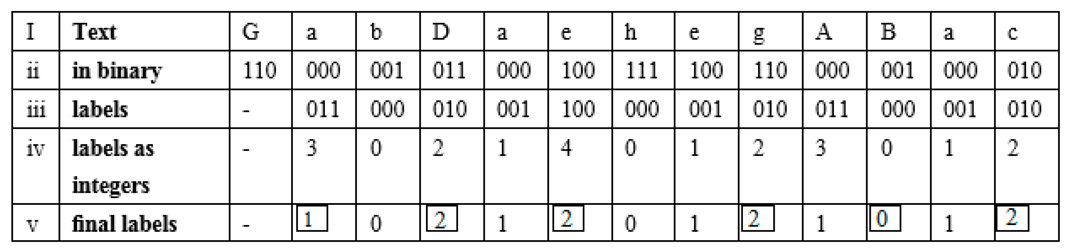
4.1. Data Embedding

We demonstrate a data-embedding scheme, which embeds data into a multidimensional matrix. Assume some data, $X$, over an alphabet, $\sum$. The data, $X$, will be embedded as $Em\left(X\right)$, an array with multi-magnitudes, $O\left(\right|\sum \left|\right|X\left|\right)$, but the number of magnitudes of the nonzero array will be relatively minimum, indeed $O\left(\right|X\left|\right)$.

The time complexity of the embedding $Em$ process is linear. The proposed scheme will parse X into different fractional data and reflect the multi-set $T\left(X\right)$ of these fractional data. We confirm that the size of $T\left(X\right)$ is as a maximum $2\left|X\right|$. Hence, $Em\left(X\right)$ is the distinguishing array for $T\left(X\right)$. The process through which the parse tree $T\left(X\right)$ will generate is known as ESP. The following subsection explores the ESP.

4.1.1. EPS

The parse tree, $EST\left(X\right)$, that is formed for data $X:X$ is the breakdown structure of partial data analogous to the nodes of $EST\left(X\right)$. The aim is to limit the data-editing operations. A clear EST contains all dynamic data of length $2^{loc}$, namely $X[lo{c}_2{2}^{loc}\dots ((lo{c}_2+1)2^{loc}-1\left)\right]\in loc$ and $lo{c}_2$; it results in a complete binary tree. However, if $X$ is updated using addition or removal to obtain $X^{\prime },X$ and $X^{\prime }$ will be construed using the same technique to two dissimilar hierarchical partial datasets; thus, the resultant embedding will not preserve approximation.

Suppose we have data $X$; the next step is to form an ESP tree in a hierarchal fashion with $P_i\left(X\right)$ repetitions. Every repetition produces a different level of EST. At every repetition, $i$, the process initiates with data, $Xi$, and divides them into chunks of size two or three. We substitute every chunk analogous to $X[lo{c}_3\dots lo{c}_2]$ by name and refer to the pair $(loc,h(X[lo{c}_3\dots lo{c}_2]\left)\right)$. Moreover, $h$ corresponds to a 1-1 hash function on partial data $X$.

Suppose $X0=X$, and the repetitions until the length of data left become 1. The EST tree of $X$ contains levels, and for every string of $Xloc-1$, a node at level $i$ must exist, and the children are the nodes in level $loc-1$. Here, a leaf node is each data unit of $X0=X$. More precisely, we can make the partitions of $Si$ data into dissimilar non-overlapping units. The data can be divided into non-overlapping units in three ways:

(a)

Maximum adjacent partial data of $Xi$ that comprise a repetitive sign ($X0$ shows in the form $a^l$ for $a\in {\mathsf{\Sigma }}_i$ where $l>1$).

(b)

Length of partial data (Long) at least ${\mathit{log}}^{*}|\sum loc-1|$ not of type 1 above.

(c)

Length of partial data (short) less than ${\mathit{log}}^{*}|\sum loc-1|$ not of type 1.

The general term “meta block” (mb) is used for all such partial data. To produce next-level parsing, we process each mb as demonstrated in the following subsections.

4.1.2. Type 2: Long Data without Duplications

We assume a dataset where two consecutive symbols are duplicates and represent an mb of type 2. Assuming a structure, $X$, without duplications (i.e., $X\left[loc\right]6=X[loc+1]$ for $loc=1\dots \left|X\right|-1$), we select as a maximum $\left|X\right|/2$ and minimum $\left|X\right|/3$ partial data of $X$ as a node. We obtain $X$ upon concatenating these nodes. The first phase comprises repeating the reduction process of an alphabet.

Reduction of alphabet ($\sum$): For every character $C\left[loc\right]$, calculate a new tag. $C[loc-1]$ is the symbol located to the left of $C\left[loc\right]$, and assume $C\left[loc\right]$ and $C[loc-1]$ are denoted as binary numbers. The least-significant bit (LSB) key where $C\left[loc\right]$ differs from $C[loc-1]$ is represented by $Le$, and assume bit ($Le,C\left[i\right]$) is the value of $C\left[i\right]$ at the $L{e}^{th}$ bit position. For example, the location of bit $Le$ is next to the character at the former index, i.e., form label ($C\left[loc\right]$) as $Le+bit(Le,C[loc\left]\right)$.

Lemma 1.

For some loc, if $C\left[loc\right]\ne C[loc+1]$, then $C\left[loc\right]\ne label\left(C\right[loc+1\left]\right)$.

Proof. 

Supposing the LSB location, where $C\left[loc\right]$ differs from $C[loc+1]$, is similar in a way where $C\left[loc\right]$ also differs from $C[loc-1]$ (else, $labelC\left[loc\right]\ne label\left(C\right[loc+1\left]\right)$). However, the bit character at this position in every symbol must be different; therefore, $labelC\left[loc\right]\ne label\left(C\right[loc+1\left]\right)$.

Adopting this method, we create an innovative series. If the existing alphabets have length, ɳ, then the extracted alphabets have size, $2\mathit{log}\left|\eta \right|$. We currently repeat (repetition is orthogonal to the duplication that produces an EST tree of $X$; repeating on $C$ that is a subseries with no matching contiguous characters) and make the character decrease until the length of the alphabet is unable to shrink. This will take ${\mathit{log}}^{*}\left|\eta \right|$ repetitions. Note that the labels for the first ${\mathit{log}}^{*}\left|\eta \right|$ symbols will not exist.

The lemma states that if a symbol at position $C\left[loc\right]$ is not equal to the symbol at position $C[loc+1]$, then the label assigned to $C\left[loc\right]$ is not equal to the label assigned to $C[loc+1]$. Lemma 1’s goal is to establish a connection between symbols and their corresponding labels based on how they differ from one another. Lemma 1’s proof demonstrates that if there is a difference between two symbols, ($C\left[loc\right]$ and $C[loc+1]$), their labels will also be different. The subsequent actions and procedures in the text are theoretically justified by this lemma. □

Lemma 2.

After the last reiteration of the $\sum$reduction, the size of $\sum$is 6.ɳ.

Proof. 

Upon every repetition of cataloguing, the size of the alphabet is reduced from $\left|\sum \right|$ to $2\left[\mathit{log}\left|\sum \right|\right]$. If $\left|\sum \right|>6$, then $2\left[\mathit{log}\left|\sum \right|\right]$ is firmly smaller than 6. A has no duplicate symbols contiguously, nor do the final order of tags on A by Lemma 1 iteratively.

Lemma 2 plays a crucial role in establishing the size of the alphabet $(\sum )$ after the last iteration of cataloguing in the given text. It states that the size of $\sum$ is 6 times the original alphabet size (ɳ) after the last repetition of cataloguing. The proof of Lemma 2 demonstrates that if the initial alphabet size is greater than 6, then the reduction process reduces the alphabet size to a value that is strictly smaller than 6.

Lastly, three passes over the order of labels were accomplished to decrease the alphabet from {0, 1, 2}: initially, we substitute every 3 with the minimum item from {0, 1, 2} that is not in the neighborhood of 3, and then we perform the same operation for every 4 and 5. This produces a series of symbols extracted from the $\sum \{\mathrm{0,1},2\}$, where no contiguous labels are equal. We designate this series $A^{\prime }$.

We currently choose distinct positions, known as landmarks, from the structures that are closely related to each other. We initially chose some location, I, and a local maximum as a landmark, such as $A^{\prime }[loc-1]<A^{\prime }\left[loc\right]>A^{\prime }[loc+1]$. □

Two local maximums might have four overriding symbols. Moreover, we chose some i as a landmark, i.e., local minima, such as $A^{\prime }[loc-1]<A^{\prime }\left[loc\right]<A^{\prime }[loc+1]$, that was not contiguous to a previously selected landmark. In Figure 2 and Figure 3, the process is depicted graphically.

Lemma 3.

For some two consecutive landmark locations,$loc$ and $lo{c}_2,2\le \left|loc-lo{c}_2\right|\le 3$.

Proof. 

Using our tagging mechanism, we claim that no contiguous pair of symbols is tagged—subsequently, we may not have two contiguous local maximums and specifically inhibit tagging local minima next to a local minimum. A modest case investigation demonstrates that the parting of landmark locations is two overriding labels. □

Lemma 4.

Defining the nearby landmark to location, $loc$, subject to only 5 adjacent locations to the right and ${\mathit{log}}^{*}\left|\eta \right|+5$ to the left.

Proof. 

Once a reiteration of alphabet reduction is performed, every symbol depends merely on its left label. We iterate this ${\mathit{log}}^{*}\left|\eta \right|$ time; therefore, the symbol at a location, $i$, is based on ${\mathit{log}}^{*}\left|\eta \right|$ for the left labels. As soon as we accomplish the last step of reducing the $\sum$ form $\sum$ of six (6) to $\sum$ of three (3), the last label at a location, $i$, is based on a max of three extra labels to its right and left. We must tag every local maximum location and, formerly, every local minimum position not contiguous to a local maximum; therefore, we must inspect max two symbols to the right of i and two labels to the left, which, in order, depends on three labels to the right and ${\mathit{log}}^{*}\left|\eta \right|+3$ labels to the left. The aggregate dependence is, hence, as indicated. We currently demonstrate how to divide A into units of size 3 or 2 nearby landmarks. □

4.1.3. Type 1 (Repeating mbs) and Type 3 (Short mbs)

We look for landmarks discovered without any difficulty in the local neighborhood. Hence, we assume data blocks containing a distinct repetitive symbol as big landmarks. Type 3 and Type 1 blocks are parsed in a usual way; the details are given for completeness. The mbs having size one are attached to the left or the right of the repeating mb. The attachment will preferably be to the left if both are possible. The mbs of size two or three are remembered as blocks without further splitting, whereas an mb of length four is allocated into two blocks of size two. In each mb with a size of five or greater, the parsing may be carried out on the leftmost three labels as a block, and then reiterate the rest.

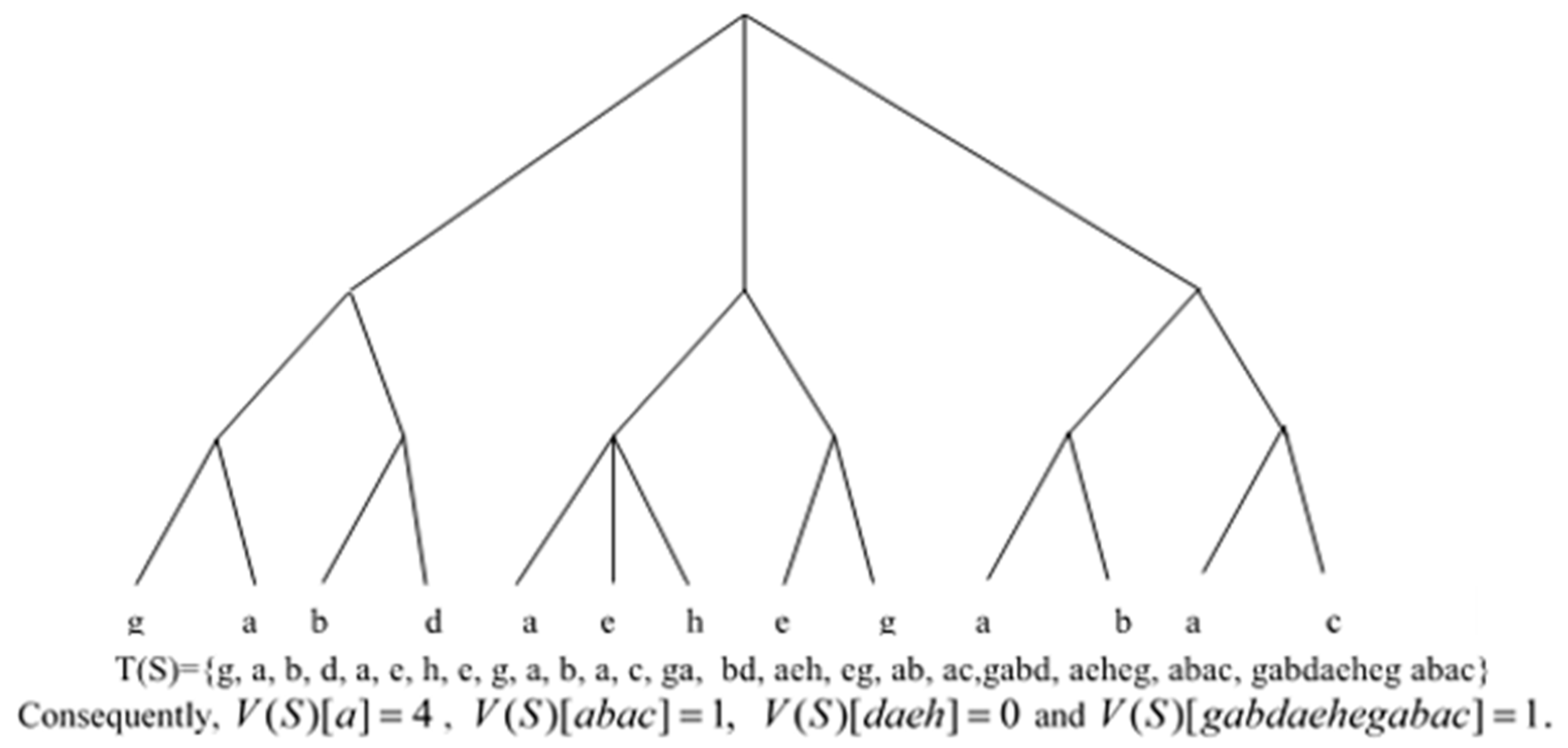
4.1.4. Constructing ET (X)

While partitioning $Xloc$ into 2 or 3 labels, $Xloc+1$ is constructed by substituting every block, $bl$, by $hf\left(bl\right)$, where $hf$ is a 1-1 naming hash function. It is essential to mention that the units of distinct levels will call hash functions onto distinct domains to compute names. To this point, the focus is on any given level $i$. Using the random property, the computation of $hf\left(\right)$ for a specific unit of size 2 or 3 will take $O\left(1\right)$ time. This produces the series $Xloc+1$; this process is reiterated till the series is of size one or till the tree root. Let $P_i\left(X\right)$ represent total nodes at level i in $ET\left(X\right)$. The original data, $M_0\left(X\right)=\left|X\right|$, are used to design the first (leaf) level from the symbols. We have $P_i\left(X\right)/3\le P_{i+1}\left(X\right)\le \left[P_i\right(X)/2]$. Hence, $\frac{3}{2}\left|X\right|\le P_i\left|X_i\right|\le 2\left|X\right|$. Therefore, for every $i$, $\left|{\sum }_i\right|\le \left|X\right|$ and, thus, ${log}^{*}\left|{\sum }_i\right|\le {log}^{*}\left|X\right|$ are shown in Figure 4.

Theorem 1.

Given the data, $X$, the $ET\left(X\right)$ can be calculated in $O(\left|X\right| {log}^{*}\left|X\right|)$ time.

4.1.5. Properties of ESP

How to calculate the$ET\left(X\right)$ for some data $X$ is defined above. Every node n in $ET\left(X\right)$ denotes the partial data of $X$ obtained from the leaf nodes on the merging in the subtree at the root node $n$.

Definition 1.

Describe the multi-set $T\left(X\right)$ such that all partial data of  $X$ are designated by the nodes of  $ET\left(X\right)$ (for each level). The characteristic array  $A\left(X\right)$ of $T\left(X\right)$, i.e., $A\left(X\right)\left|n\right|$, can be defined as the sum of occurrences a partial data $n$ appears in $T\left(X\right)$. In conclusion, $A_i\left(X\right)$ the features array limited to those nodes appear at a level $i$ in $ET\left(X\right)$.

$T\left(X\right)$ contains as a maximum $2\left|X\right|$ data having size $\left|X\right|$ An (X) is $O(\left|\sum \right|+\left|X\right|)$ dimensional array as its dominion is some data that exist in $T\left(X\right)$.

The typical $L_1$ distance between two arrays $a_1$ & $a_2$ by $\left|\left|a_1-a_2\right|\right|1$ is specified. $‖A\left(X\right)-A\left(Y\right)‖1=P_{X\in T\left(X\right)\cup T\left(Y\right)}\left|A\left(X\right)\left[x\right]\right.-\left.A\left(Y\right)\left[x\right]\right|$. Recall that $d(X,Y)$ indicates the match with moves among data Y and X.

Theorem 2.

For data $Y$ & $X$, suppose $n$ be maximum $(\left|Y\right|,\left|X\right|)$. Then $‖A\left(Y\right)-A\left(X\right)‖1=O\left(\mathit{log}n{\mathit{log}}^{*}n\right)d(X,Y)$.

4.2. Upper Bound Proof $‖A\left(Y\right)-A\left(X\right)‖1=O\left(\mathit{log}n{\mathit{log}}^{*}n\right)d(X,Y)$

Proof. 

Express this bound on $L1$ space, assume the impact of the edit procedures, and show that all adds a role to the $L1$ distance limited by $O\left(\mathit{log}n{\mathit{log}}^{*}n\right)$. Editing processes are permitted to overlay on blocks. We present a Lemma applicable to all data, except with no contiguous repetitive alphabets. □

Lemma 5.

The nearby landmark to any character of $X_{loc}$ is computed by at most five successive characters of $X_{loc}$ to the right and at most ${\mathit{log}}^{*}\left|{\Sigma }_{loc}\right|+5$ repeated characters of $X_i$ to the left.

Proof. 

Assume that a character of $X_{loc}$, i.e., $X_{loc}\left[lo{c}_2\right]$, indicates the mechanism to identify the nearby landmark.

Type 1 Iterating mb: A lengthy duplication of a character, $c$, is considered a distinct and larger landmark. $X_{loc}\left[lo{c}_2\right]$ is contained within such an mb if $X_{loc}\left[lo{c}_2\right]=X_{loc}[lo{c}_2+1]$ or if $X_{loc}\left[lo{c}_2\right]=X_{loc}[lo{c}_2-1]$. We also assume $X_{loc}\left[lo{c}_2\right]$ to be part of a reiterating partial data if $X_{loc}[lo{c}_2-1]=X_{loc}[lo{c}_2-2];X_{loc}[lo{c}_2+1]=X_{loc}[lo{c}_2+2];$ and $X_{loc}\left[lo{c}_2\right]6=X_{loc}[lo{c}_2+1]$ and $X_{loc}\left[lo{c}_2\right]6=X_{loc}[lo{c}_2-1]$.

Type 2 and type 3 Nonrepeating mbs: When $X_{loc}\left[lo{c}_2\right]$ is not a character in re-counting mb, formerly choose it either in a long or short mb. We investigate the partial data $X_{loc}[lo{c}_2-\mathit{log}\ast \left|{\Sigma }_{loc}\right|-3\dots lo{c}_2-1]$. When there is a $k$ such that $X_{loc}\left[lo{c}_3\right]=X_{loc}[lo{c}_3-1]$ and $lo{c}_3$ is more significant than all, a repeating mb ending at location $lo{c}_3$ exists. In the landmark, thus, we analyze $X_{loc}\left[lo{c}_2\right]$ as a short mb part, beginning at $X[lo{c}_3+1]$. Inspecting the partial data $X[lo{c}_2+1\dots lo{c}_2+5]$ permits us to find if there is an additional repeating mb nearby location, $lo{c}_2$, and we can decide the formation of a node comprising $X_{loc}\left[lo{c}_2\right]$. When no repeating mb is marked in $X_{loc}[lo{c}_2-{\mathit{log}}^{*}\left|{\Sigma }_{loc}\right|-3\dots lo{c}_2-1]$, it is possible to use the alphabet decrease procedure to find a landmark. The ability to find a nearby landmark to a character through observing only a limited number of successive nearby codes demonstrates that if a modification occurs outside this area, a similar landmark will be found; hence, a similar node will be shaped comprising that symbol. This permits the verification of the subsequent lemma. □

Lemma 6.

Inserting $lo{c}_3\le {\mathit{log}}^{*}n+10$ contiguous symbols into $X$ to obtain $X^{\prime }$ means $‖A_i\left(X\right)-A_i\left(X^{\prime }\right)‖1\le 2({\mathit{log}}^{*}n+10)$ Є levels.

Proof. 

We have a contribution after the insertion itself into the $L1$ distance and its effect on the nearby vicinity. Assume that the aggregate of characters at the level $i$ break down to distinct nodes next to addition equated to earlier nodes. Consider the total characters at a level $i$ break down in a different way as a result of the insertion $P_i$. Lemma 4.5 proves that in a non-overlapping mb, any character ${\mathit{log}}^{*}\left|{\mathsf{\Sigma }}_{loc}\right|+5$ indexes to the right or above five indexes to the left of each character can be altered and will identify the identical nearby landmark; hence, it will be shaped according to similar nodes. Hence, it will not pay for $P_i$. In the same way, for an overlapping mb, any character within the block will be parsed into a similar node (i.e., into a tripartite of that character), excluding the last four characters and depending on the block size.

Thus, for an overriding mb, $P_i\le 4$. The total characters that are lower-level parsed in a different way into nodes as a result of the insertion are max $P_i-\frac{1}{2}$, and there is an area of 5 characters at maximum to the left, plus ${\mathit{log}}^{*}\left|{\mathsf{\Sigma }}_i\right|+5$ characters on the right side are parsed differently at a level $i$. As noted earlier, $\left|{\mathsf{\Sigma }}_i\right|\le \left|X\right|\le n$, and the recurrence $P_i\le P_i-\frac{1}{2}+{\mathit{log}}^{*}n+10$ can consequently form. If $P_i-1\le 2({\mathit{log}}^{*}n+10)$, then $P_i\le 2({\mathit{log}}^{*}n+10)$. Insertion point, $P_0\le {\mathit{log}}^{*}n+10$. To conclude, $‖A_i\left(X\right)-A_i\left(X^{\prime }\right)‖1\le 2(P_i-\frac{1}{2})$, so then we might miss $P_i-\frac{1}{2}$ ancient nodes and obtain these various new nodes. □

Lemma 7.

Removing $k<{\mathit{log}}^{*}n+10$ contiguous characters from  $X$ to obtain $X^{\prime }$ means $‖A_i\left(X\right)-A_i\left(X^{\prime }\right)‖1\le 2({\mathit{log}}^{*}n+10)$ .

Proof. 

Notice that the removal of a series of symbols is exactly the double to addition of that series at the similar index. Assume that a series of symbols pop in and then are removed; the resulting data are the same as the original data. Hence, the modified nodes number must be essentially limited by its equal quantity to the insert, as proved in Lemma 6. We merge both lemmas to confirm that modifying processes limited the parse-tree influences. □

Lemma 8.

When a particular allowed operation of edit distance alters data $X$ to $X^{\prime }$, then $‖A\left(X\right)-A\left(X^{\prime }\right)‖1\le 8\mathit{log}n({\mathit{log}}^{*}n+10)$.

Proof. 

Each permissible procedure is assumed.

Character edit processes

The scenario for inserting follows straightaway from Lemma 6, as the character insertion operation will influence the breakdown of max $2({\mathit{log}}^{*}n+10)$ characters at all levels and the maximum levels $\mathit{log}2n.$ Overall, $‖A\left(X\right)-A\left(X^{\prime }\right)‖1\le 2\mathit{log}n({\mathit{log}}^{*}n+10)$. Likewise, the scenario for deletion follows instantaneously from Lemma 7. To conclude, the case for substitution is presented by noticing that a symbol substitution assumed that can be used for removing instantly contiguous to an addition.

Partial data Moves

If the size of partial data being moved is ${\mathit{log}}^{*}n+10$ at maximum, then a move can be said to be a deletion of the partial data following its reinsertion somewhere else. From Lemma 6 and Lemma 7, we see that $‖A\left(X\right)-A\left(X^{\prime }\right)‖1\le 4\mathit{log}n({\mathit{log}}^{*}n+10)$. Otherwise, we assume parsing of partial data by ESP. Assume a symbol in a non-iterating mb greater than ${log}^{*}+5$ symbols from the beginning of partial data and greater than 5 symbols from the tail. As per Lemma 5, only symbols inside the partial data being moved decide how that symbol is parsed. Therefore, the parsing of these symbols and, hence, the contribution to $A\left(X\right)$ are free of the position of partial data in original data. Only the ${\mathit{log}}^{*}n+5$ symbols at the start and 5 symbols of the partial data at the end will influence the data-parsing procedure. We can consider these to be the deletion of two partial data of the size $k\le {\mathit{log}}^{*}n+10$ and their reinsertion somewhere else.

Lemma 8 demonstrates that each permissible action influences the $L1$ conversion distance by $8\mathit{log}n({\mathit{log}}^{*}n+10)$ maximum. Assume we initiate with $Y$ and accomplish a sequence of $d$ editing processes, generating $Y_1,Y2,\dots Y_d$ as a result. To conclude, $Y_d=X$, so $‖A\left(Y_d\right)-A\left(X\right)‖1=0$. We start with a number, $‖A\left(Y\right)-A\left(X\right)‖1$; in addition, we are aware that $‖A\left(Y_{lo{c}_2}\right)-A\left(Y_{lo{c}_2+1}\right)‖\le 8\mathit{log}n({\mathit{log}}^{*}n+10)$ was discussed above. Henceforth, as $d(X,Y)$ steps, convert $Y$ to $X$, and then $‖A\left(Y\right)-A\left(X\right)‖\frac{1}{8}\mathit{log}n({\mathit{log}}^{*}n+10)\le d(X,Y)$, giving around $d(X,Y).8\mathit{log}n({\mathit{log}}^{*}n+10)$. □

4.3. Data Aggregation Level 2 Problem Solution

In this subsection, an algorithm is proposed that solves the problem of DMM. For any data $X$, we adopt that $A\left(X\right)$ needs to be placed in the space of $O\left(\left|X\right|\right)$ via registering nonzero parts only of $\left|X\right|$. Furthermore, appropriately, we save $A\left(X\right)\left[x\right]$ as an array indexed by $h\left(x\right)$ if it is nonzero, and we hold $x$ as a reference to $X$, along with $\left|x\right|$.

The following outcome on pairwise data association is tracked directly from Theorems 1 and 2 composed with the surveillance that is given: $A\left(Y\right)$ and $A \left(X\right)‖A\left(Y\right)-A\left(X\right)‖1$ found in $O(\left|Y\right|+\left|X\right|)$ time.

Theorem 3.

Given data $X$ and $Y$ with $n=max\left(\left|X\right|,\left|Y\right|\right)$, to approximate a deterministic algorithm used for $d\left(X, Y\right)$ to precise up to an $O\left(\mathit{log}n{\mathit{log}}^{*}n\right)$ factor in $O\left(n{\mathit{log}}^{*}n\right)$ time with $O\left(n\right)$ space.

4.3.1. Pruning Lemma

Before solving the data-match problem, pattern p of size m associate with $t[loc\dots n]$ for each $i$, then there will be $O\left(n\right)$ comparisons. Moreover, we have to calculate the distance among $p$ and $t[loc\dots lo{c}_3]$ for all possible $lo{c}_3\ge loc$ to calculate the optimal placement beginning at the location $i$, that shows sub-problems generally $O\left(mn\right)$. In the worst case, the algorithm of classical dynamic programming accomplishes the whole evaluations in $O\left(mn\right)$ time at max by using the dependency between sub-problems. In the algorithm, a different methodology is proposed. Initially, the below crucial observations were made:

Lemma 9.

(Pruning Lemma) Given an arrangement, t, and string, $s$, $\forall loc,lo{c}_2:1\le loc\le lo{c}_2\le n, d(t,s[loc\dots loc+m-1]\le 2d(t,s[loc\dots lo{c}_2])$.

Proof. 

Note that for all $j$ values in lemma, $d(t,s[loc\dots lo{c}_2\left]\right)\ge \left|(Y-loc+1)-m\right|$, as these multiple symbols must be deleted or inserted. By triangle inequality of match with moves, for all, $lo{c}_{2}d(t,s[loc\dots loc+m-1]$.

$$\begin{array}{c}\le d\left(t,s\left[\mathit{loc}\dots lo{c}_2\right]\right)+d(s\left[\mathit{loc}\dots lo{c}_2\right],s\left[\mathit{loc}\dots \mathit{loc}+m-1\right]\hfill \\ \hspace{1em}=d\left(t,s\left[\mathit{loc}\dots lo{c}_2\right]\right)+\left|\left(Y-\mathit{loc}+1\right)-m\right|\hfill \\ \le 2d\left(t,s\left[\mathit{loc}\dots lo{c}_2\right]\right)\hfill \end{array}$$

The lengthiest common prefix followed to assume $s\left[\mathit{loc}\dots lo{c}_2\right]$ and $s\left[\mathit{loc}\dots \mathit{loc}+m-1\right]$.

The above Lemma importance is that it serves to estimate only $O\left(n\right)$ distances, such as $d(t,s\left.\mathit{loc}\dots \mathit{loc}+m-1\right)$ for all $i$ values, to solve the data-match problem DMM, equal to a factor 2 approximation. Therefore, it trims away candidates from the “quadratic” number of distance calculations that an honest process would require. □

4.3.2. ESP Sub-Trees

We estimate distance among partial data s and the pattern t by matching the parsing ESP of two patterns. On the other hand, it would be costly and useless to parse the partial data s. In this subsection, we indicate that an ESP tree is assigned to a datum, and being inspired by a partial datum means that the subtree will have similar editing sensitivity features as the complete one.

Definition 2.

Let $E{T}_{loc}{\left(X\right)}_{lo{c}_2}$ at $lo{c}_2$, such that loc represents the level of UAV in the breakdown of $X$.

The set of values $X\left[a_1\dots a_n\right]$ to the tags on last level of the sub-tree, where (root) $E{T}_{loc}{\left(X\right)}_{lo{c}_2}$ is defined as range, $\left(E{T}_{loc}{\left(X\right)}_{lo{c}_2}\right)$, and relates to the partial data, $X\left[a_1\dots a_n\right]$.

The ESP subtree of data $X$ can be defined $EST\left(X,l,r\right)$ as the sub-tree $ET\left(X\right)$ that comprises all $X\left[loc\right]$, such that $l\le \mathit{loc} \le r$, plus all parent UAVs. Formally, we search and discover UAVs of $E{T}_{loc}{\left(X\right)}_{lo{c}_2}$, where $\left[l\dots r\right]\cap range\left(E{T}_{loc}\left(X\right)lo{c}_2\right)6=\mathrm{\varnothing }.$ A name node is derived from $E{T}_{loc}{\left(X\right)}_{lo{c}_2}$, which is $loc,hX\left.range\left(E{T}_{loc}\left(X\right)lo{c}_2\right)\cap \right[a\dots b\left)\right)$.

This results in an appropriate sub-tree of $ET\left(X\right)$, as a node is part of the sub-tree if one of its children is counted in as a minimum. As stated earlier, we can define an array that represents this $ET$.

Definition 3.

Define $AX\left(X, l, r\right)$ as the characteristic array of $EST\left(X\right)$ by similarity with $A\left(X\right)$; namely $AX\left(X, l, r\right)\left[x\right]$ represents the the total times the partial data x are denoted as a node in $EST\left(X, l, r\right)$. In this regard, $EST\left(X, 1, \left|X\right|\right)=ET\left(X\right)$; however, if not, generally $EST\left(X, l, r\right)=ET\left(X\left[l\dots r\right]\right)$. Through $EST\left(X, l, r\right)$, it send the features of the edit-sensitive parsing. Similar to Theorem 2, Theorem 4 is stated as follows.

Theorem 4.

Let $d$ be $d\left(Y\left[l_p\dots r_p\right], X \left[l_q\dots r_q\right]\right)$. Then, $d\le 2\left|\left|A.XY, l_p, r_p)-A X(X, l_q, r_q\left]\right)\right|\right|1=O\left(logn{ log}^{*}n\right)d$.

Proof. 

Definitely, as Lemma 9 does not assume anything regarding the tree structure, the lower bound exists, meaning that the edit distance is simply double the length of the difference amongst the ESP subtrees.

For the higher limit, assume implementing the required editing processes to the partial data of $X$ and $Y$. The impact on the ordinary ESP trees is observed, $ET\left(Y\right)$ and $ET\left(X\right)$. Theorem 2 verified that all editing processes could create a divergence of $O\left(logn{log}^{*}n\right)$ maximum among $A\left(X\right)$ and $A\left(X^{\prime }\right)$. Following this, the variance in $AS\left(X,l,r\right)$ should be limited as a result of similar volume: it seems impossible to remove additional UAVs, as the UAVs of $EST\left(X,l,r\right)$ is the subset of UAVs of $ET\left(X\right)$. Hence, as demonstrated in Theorem 2, the aggregate divergence $\left|\left|A.X\left(Y,l_p,r_p\right)-A.X\left(X,l_q,r_q\right)\right|\right|1=d·O\left(logn{log}^{*}n\right)$. □

Lemma 10.

$A X\left(X, l+1, r+1\right)$ can be calculated from $A X\left(X, l, r\right)$ in time $O\left(log \left|X\right|\right)$.

Proof. 

Remember that a UAV is contained within $EST\left(X,l,r\right)$ once any dependent is last-level analogous to $X\left[i\right]$ contained when $i\in \left[l\dots r\right]$. It results in an easy method for discovering $EST\left(X,l+1,r+1\right)$ from $EST\left(X,l,r\right)$ and $AX\left(X,l+1,r+1\right)$. We need to eliminate $X$ and some parents that do not cover $X\left[l\right]$ from $EST\left(X,l,r\right)$ to generate $AX\left(X,l+1,r+1\right)$.

Each parent $X$ is adjusted to guarantee that its tag is accurate. The UAV located at i(level) matching to the partial data $X\left[lo{c}_2\dots lo{c}_3\right]$, which is a parent of $X$, was earlier denoted in the sub-tree via the $\left(loc,h\left(X\left[l\dots lo{c}_3\right]\right)\right)$; it is required to be substituted with $\left(loc,h\left(X\left[l+1\dots lo{c}_3\right]\right)\right)$.

Suppose y is a UAV conforming to $X\left[r+1\right]$ in $ET\left(X\right)$ at the right. We add $y$ to $EST\left(X,l+1,r\right)$ to generate $EST\left(X,l+1,r+1\right)$, and we give the ancestor of $y$ and designate her ancestor in $ET\left(X\right)$; give her the parent addition of your choice when it is absent. Alter each parent of $y$ to guarantee that their name is accurate: a parent of $y$ corresponding to the data $X\left[lo{c}_2\dots lo{c}_3\right]$ will set $\left(loc,h\left(X\left[lo{c}_2\dots r+1\right]\right)\right)$. As these circumstances, we simply assume parents of a child UAV since the depth of tree is $O\left(log\left|X\right|\right)$, and this shows that the process complexity with respect to time is $O\left(log\left|X\right|\right)$. □

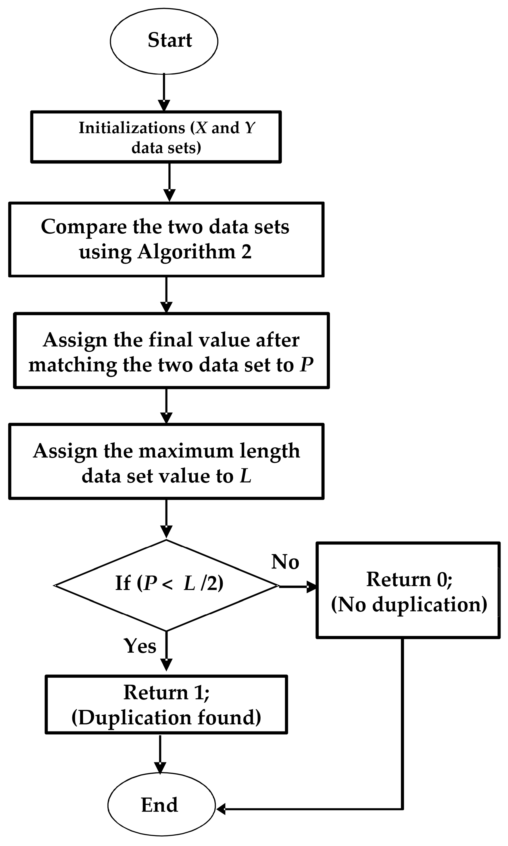
4.4. Data Aggregation Level 2 Algorithm

Theorem 5.

Given a text, $t$, and string $s$, to resolve the data-matching issue with moves by calculating an $O(log n {log}^{*}n)$ approximation to $D\left[loc\right]=min\_loc\le lo{c}_3\le n d\left(s, t\left[\mathit{loc}\dots lo{c}_3\right]\right)$ for each $loc$ in time $O\left(n log n\right)$.

Proof. 

Our algorithm is as follows:

Given a dataset $X$ of size m and dataset $Y$ of size $n$, we calculate $ET\left(s\right)$ and $ET\left(t\right)$ in time $O\left(m{log}^{*}n\right)$ as per Theorem 1.

Measure $EST\left(t,1,m\right)$. This can be performed in the $O\left(n\right)$ worst case, as a pre-order traversal of $ET\left(t\right)$ will be performed to determine which nodes are in $EST\left(t,1,m\right)$. From this, we can calculate $\widehat{D}\left[1\right]\left|\left|AX\left(t,1,m\right)-AX\left(p,1,m\right)\right|\right|1$. We then recursively calculate $\left|\left|AX\left(t,\mathit{loc}+1,\mathit{loc}+m\right)-AX\left(s,1,m\right)\right|\right|1$ from $\left|\left|AX\left(t,\mathit{loc},\mathit{loc}+m-1\right)-AX\left(s,1,m\right)\right|\right|1$ via Lemma 7 to discover which nodes we need to add to or remove from $EST\left(t,loc,loc+m-1\right)$ and regulate the total of the difference properly. □

This requires n comparisons and will take $O\left(logn\right)$ time for each. By Theorem 4 and Lemma 9, $D\left[loc\right]\le \widehat{D}\left[loc\right]\le O\left(logn{log}^{*}n\right)D\left[loc\right]$. If $logn$ is $O\left(logm\right)$, as one would expect for some rational size string and text, then a tighter investigation demonstrates the running time to be $O\left(nlogm\right)$. This is for the reason that we merely want to assume the lower $logm$ levels of the parse trees; above, this $EST\left(t,loc,loc+m-1\right)$ has only one node in each level. Figure 5 shows the flow of data aggregation Algorithm 2 to find the duplicated data in two datasets, X and Y.

Algorithm 2: Data Aggregation Algorithm to Find the Duplicated Data in Two Datasets, X and Y
Procedure Data_Match_with_Moves (DMM)
Input: Datasets, X and Y
Output: True/False // Duplication Found or Not Found
1.	Initializations Xlen ← X.length() Ylen ← Y.length ()
2.	Allocate vector space V[0:m, 0:n] ▷ V[i, j] will contain the length of X[1:i] and Y[1:j].
3.	V[0, j] ← 0 for all 0 ≤ j ≤ n and V[i, 0] ← 0 for all 0 ≤ i ≤ m. ▷ Base Cases
4.	for (i ← 1 to Xlen) then
5.	for (j ← 0 to Ylen) then // matching the symbols from X with Y symbols
6.	if (j = 0) then // if Y is blank then eliminate all X symbols // if symbol from both dataset is matching then no operation is required
7.	V[i % 2][j] ← i;
8.	else if (X[j − 1] = Y[i − 1]) then
9.	V[i % 2][j] ← V[(i − 1) % 2][j − 1];
10.	end else if // if symbols from both datasets do not match, then we take the smallest from 3 operations. // i.e., insert, delete and substitute
11.	else then
12.	V[i % 2][j] ← 1 + min(V[(i − 1) % 2][j],
13.	min(V[i % 2][j − 1],
14.	V[(i − 1) % 2][j − 1]));
15.	end if
16.	end for
17.	end for // after filling the V vector, if the size of Xlen is even, then //we end up in the 0th row else //we end up in the ith row, so we take Xlen % 2 to get row
18.	P←V[Xlen % 2][Ylen] // the final value after matching two datasets
19.	L←max (Xlen, Ylen)
20.	if (P < L/2), then
21.	return 1 // true value will return, i.e., duplication found
22.	else then
23.	return 0 // false value will return, i.e., duplication not found
24.	end if
25.	end procedure DMM

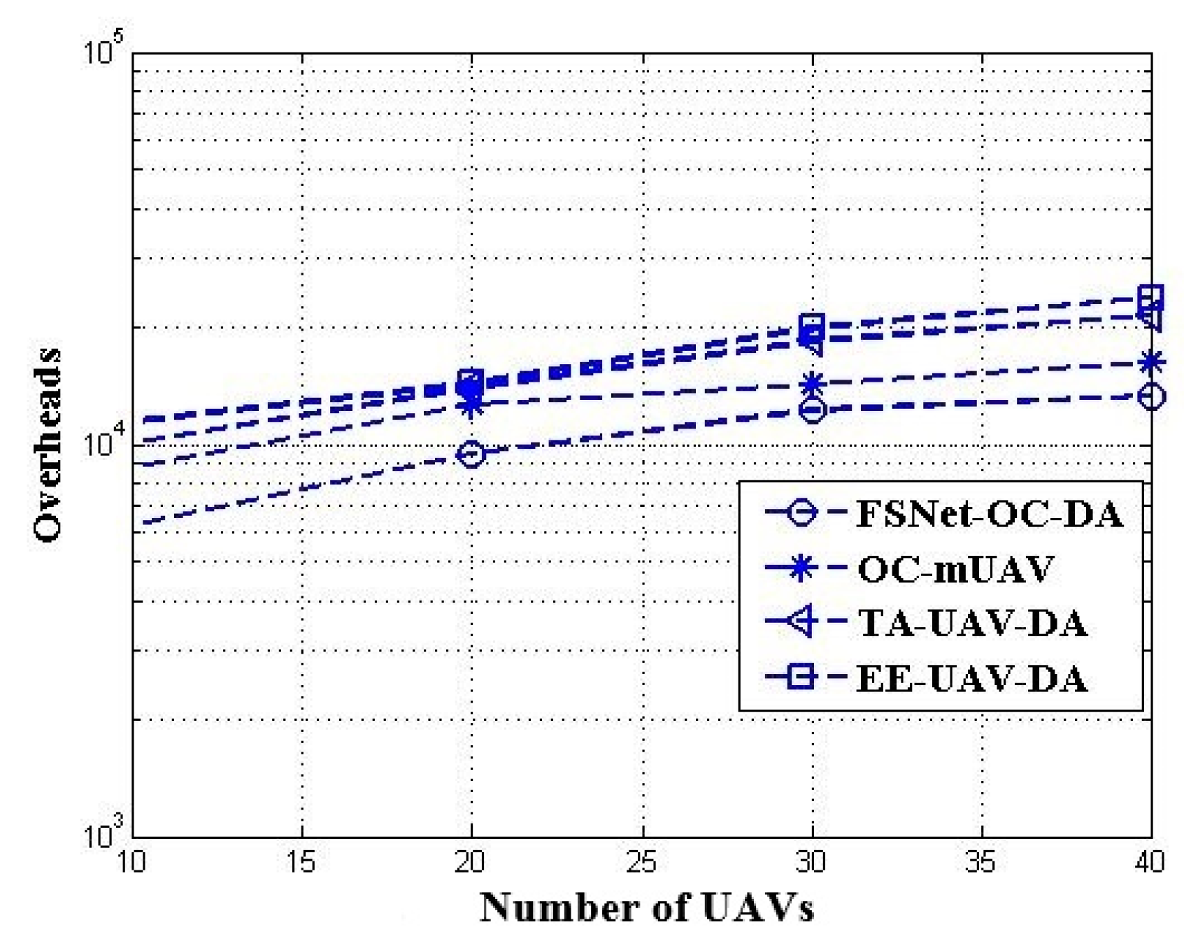
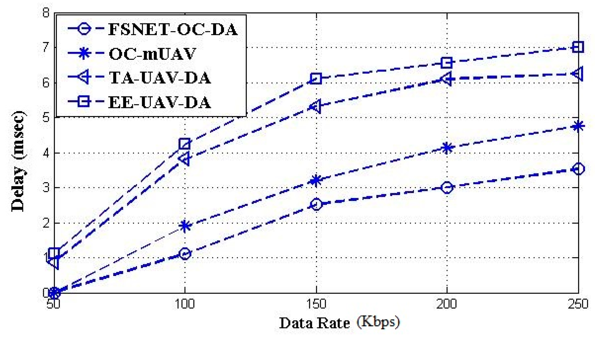
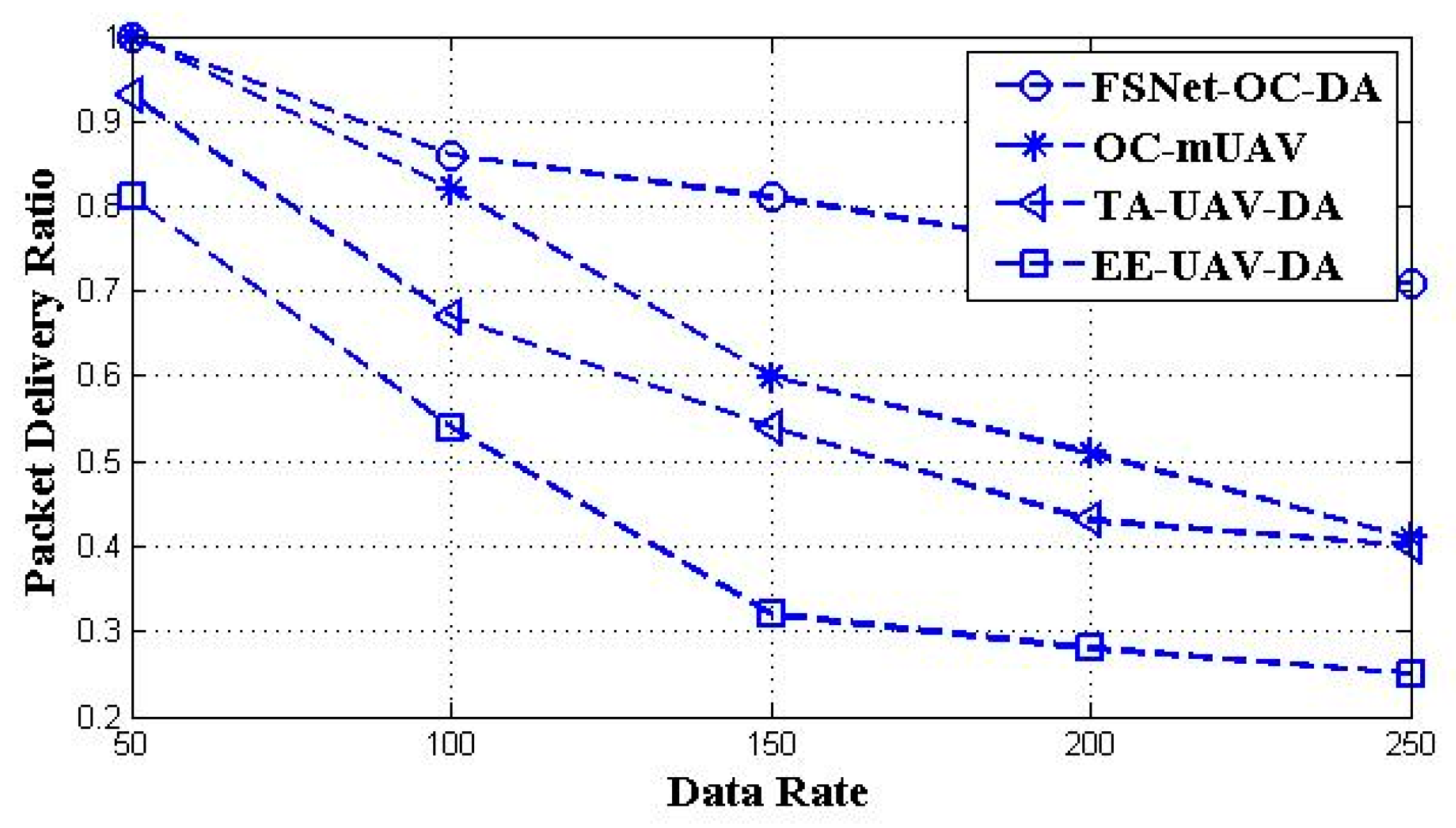
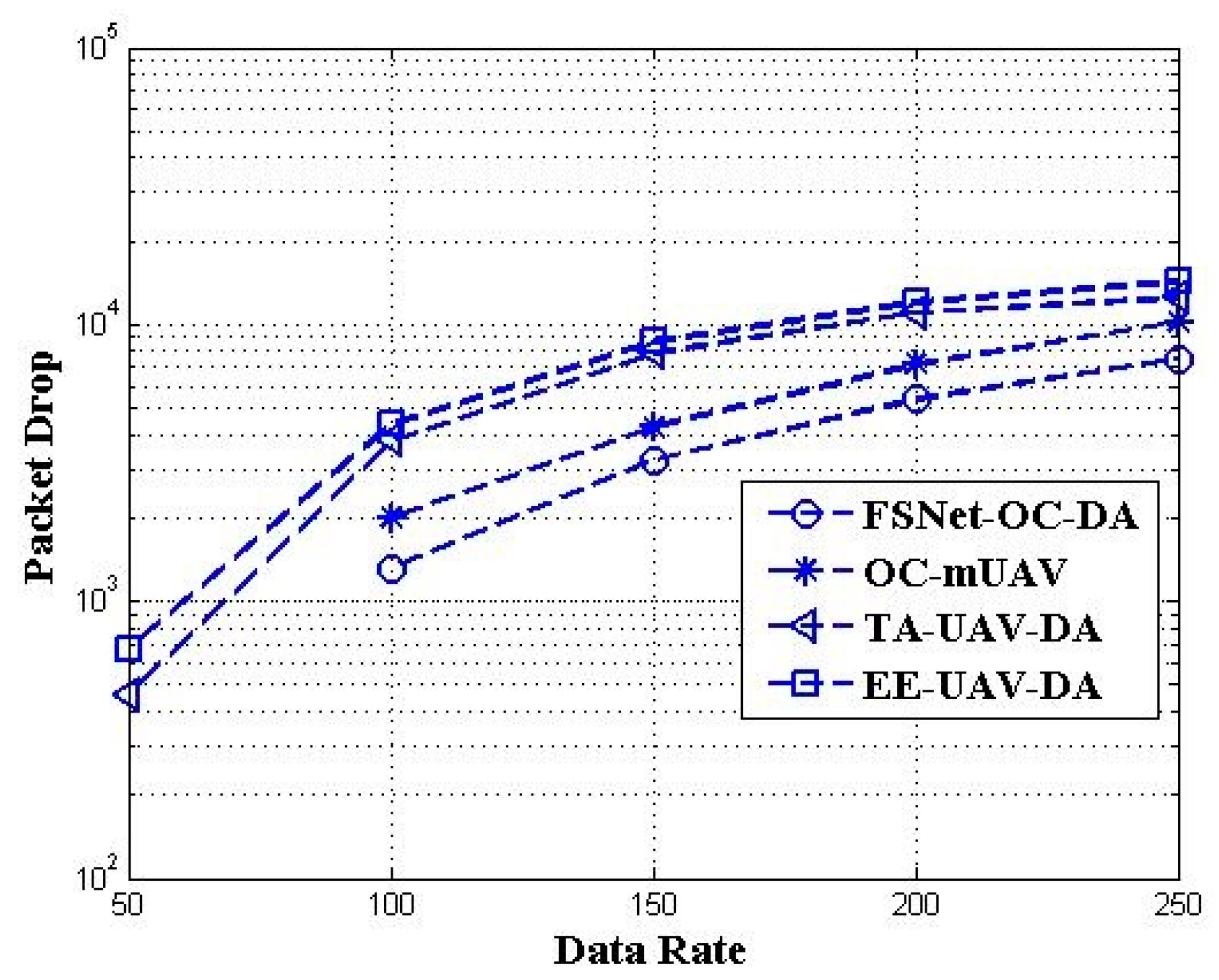
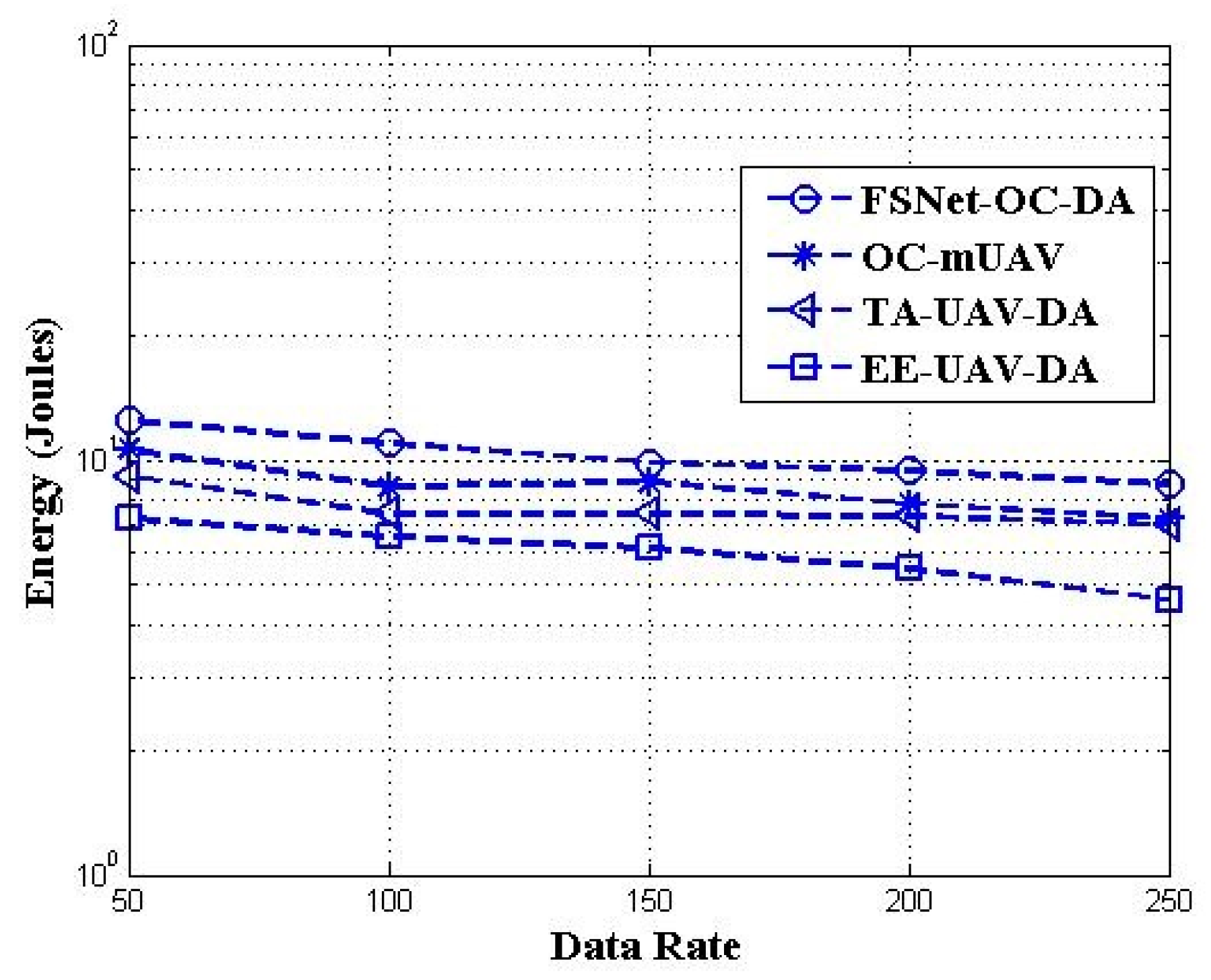
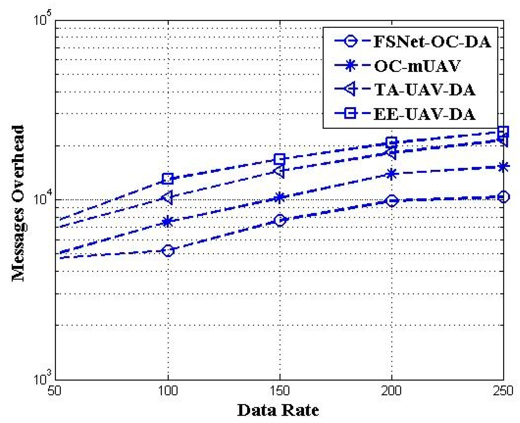
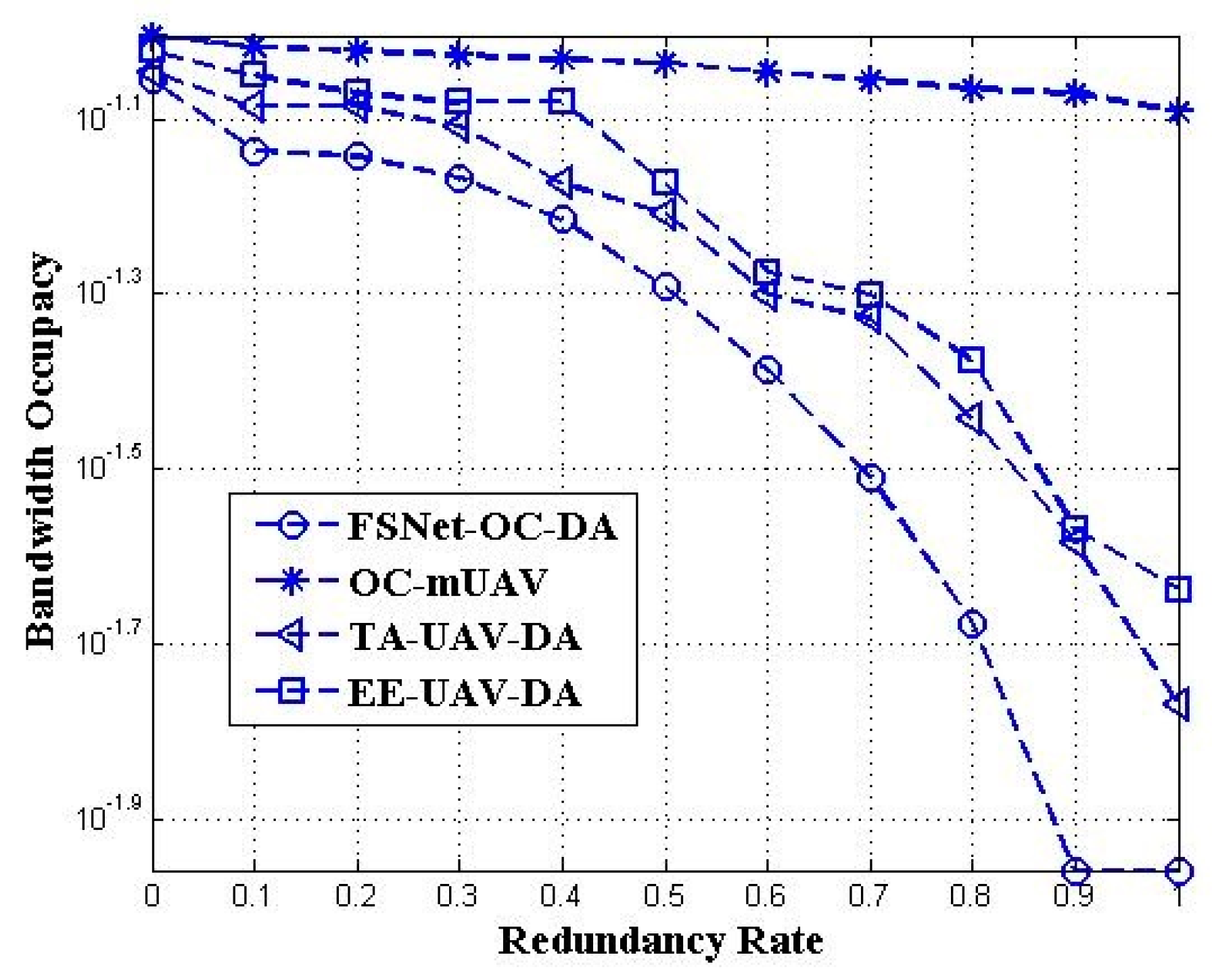
5. Performance Evaluation and Simulation Study

The performance metrics for evaluating the proposed scheme were measured with the mean packet delivery ratio (PDR), mean energy consumption, end-to-end delay, packets drop ratio, communication overhead, and bandwidth utilization [41,42,43]. The PDR is the ratio of packets received by the receiver UAVs versus the packet sent by the sender UAVs. The higher ratio means that the performance of the proposed scheme is better. The energy consumption shows the mean amount of energy consumed by the UAVs for data transmission. The end-to-end delay means the time taken by the UAVs for packets’ sending and receiving. It also measures the delay caused during route discovery and waiting in a queue. The packet drop ratio means that the packets may be dropped during the transmission, and it counts the ratio of the total number of packets received and packets sent. Sometimes, the same packets or the additional information communicated to the UAVs-CH reduces communication speed and consumes energy. The details of the simulation parameters are given in

Table 1. Simulation parameters.

Parameter	Value
Network Simulator	MATLAB
Covered Area	2 km × 2 km
MAC Protocol	IEEE 802.11 and IEEE 802.16
Antenna Type	Omni directional
Propagation Model	Two-ray ground reflection model (intra-cluster) Long-distance propagation loss model (inter-cluster)
Radio Frequency	2.4 GHz, 5 GHz
Number of UAVs	10 to 60
UAV Altitude	40–50 m
UAV Transmission Range	200 to 300 m
UAV Mobility Model	Random waypoint model
Transport Protocol	Stream control transmission protocol (SCTP)
Traffic Model	Poisson traffic model
Application Packet Size	1000 Bytes
Initial Energy	2 to 5 J
Channel Model	Multi-Propagation Channel (MPC) Model

.

The performance of the proposed redundant data elimination aggregation approach was compared with non-redundant data elimination aggregation approaches, i.e., EE-UAV-DA, OC-mUAV, and TA-UAV-DA. The data rate was fixed in the simulation, i.e., 250 Kbps, and the number of UAVs varied from 10 to 60.

Figure 6 shows the number of UAVs and the mean end-to-end delay. It is observed that with the increase in UAVs, the proposed scheme has less of a mean delay as compared to the EE-UAV-DA, OC-mUAV, and TA-UAV-DA. The FSNet-OC-DA uses HBA to form clusters and data aggregation. Selecting optimized cluster heads has a strong impact on end-to-end delay. The results show that our proposed scheme (FSNet-OC-DA) performs better than other schemes under consideration.

Figure 7 presents the number of UAVs vs. PDR. The simulation results show that, initially, the PDR decreased with an increase in UAVs. The PDR of the proposed scheme falls, while the EE-UAV-DA, OC-mUAV, and TA-UAV-DA have more decreases than our proposed algorithm. The impact of optimum cluster formation using HBA reflects that once optimized cluster heads are selected, this will increase the PDR. This is because the cluster heads belong to optimal zones with high energy, relative mobility, and high density. As the packets are routed via cluster heads, the proposed scheme with optimal cluster heads performs better than others.

Figure 8 illustrates the number of UAVs and packet drop ratio of the proposed scheme and other existing approaches. The simulation result shows that the drop ratio increased in the existing methods and our proposed scheme with the increase in UAVs. The packet drop ratio increased in all schemes because, in dense networks, the number of packets increases, and the load on other nodes also increases. This results in packet drops because the nodes are overloaded. The packet drop in our proposed scheme is less than others because we optimized cluster formation using HBA.

The increase in the number of UAVs has a direct impact on residual energy. Figure 9 shows that the proposed FSNet-OC-DA residual energy (recorded in round 10) is better than all existing approaches. The proposed scheme eliminates duplicate data transmission to the UAVS-CH by using a near-linear time algorithm. Eliminating data reduces long-distance communication. As we already know, communication consumes more energy than computation. Our model focuses on optimization and reduces communication costs. The efficient optimization and data aggregation enable nodes to consume less energy. Hence, FSNet-OC-DA energy consumption is better than the other schemes.

Figure 10 shows that the communication overhead increases with the increase in UAVs, but the FSNet-OC-DA has significantly less communication overhead. The number of UAVs in each cluster is fixed in the simulation, i.e., 40, and the data rate varies from 50 to 250 Kbps. Figure 11 represents the UAVs’ data rate and end-to-end delay of the FSNet-OC-DA, EE-UAV-DA, OC-mUAV, and TA-UAV-DA. The simulation result in Figure 10 shows that the end-to-end delay increases with the increase in data rates from 50 to 250 Kbps. It is observed that the FSNet-OC-DA has less end-to-end delay than the existing approaches. The PDR for different data rates (50 to 250 Kbps) is represented in Figure 12. Initially, when the data rate is 50 Kbps, the PDR is very high, but the delivery ratio decreases gradually with the increase in the data rate.

Figure 13 shows that, initially, the UAVs’ data rate is 50 Kbps, and the packet drop ratio is very minimal. Still, with the increase in the UAVs’ data rate, the packet drop ratio increases up to the highest level. The FSNet-OC-DA packet drop ratio is always lower when the data rate varies from 50 to 250 Kbps.

Figure 14 represents the data rate and residual energy of UAVs. The residual energy decreases with the increase in the data rate of UAVs. The remaining residual energy of the FSNet-OC-DA is still better among other existing approaches.

Figure 15 represents the UAVs’ data rate and the ratio of the message overhead. The non-redundant data elimination approaches’ communication overhead is higher than the proposed redundant data elimination schemes. Bandwidth is the capacity of communication channels among the UAVs. The bandwidth occupancy rate is the ratio of the bandwidth used by the redundant data elimination aggregation approach and without redundant aggregation approaches.

Figure 16 represents the bandwidth occupancy and redundancy rate of each UAV. The bandwidth occupancy of the FSNet-OC-DA is moving towards close to zero compared to the existing approaches. In FSNet-OC-DA, the UAVs avoid redundant data and transmit only actual data to a UAVS-CH. At the same time, the conventional data aggregation approaches utilize (50) percent bandwidth of the total available bandwidth.

6. Conclusions and Future Work

Sensors and UAVs have made it easier to monitor, observe, and share information about an area of interest remotely. The researchers proposed energy-efficient schemes by considering different parameters, such as reducing communication distance, computation cost, mobility, and degree. However, data collection minimizes the communication load to save bandwidth and energy.

In this study, the honeybee foraging property was first used to select the optimal CH set and form stable and balanced clusters. The modified HBA selects UAVs-CH based on residual energy, UAV degree, and relative mobility. To transmit data, the UAV connects to the nearest CH. Ordinary UAVs choose CH randomly if they have the same distance with more than one CH. The reaffiliation rate will decrease with the proposed stable clustering procedure. Secondly, ordinary UAVs transmit data to their CH once clusters are formed. An aggregation method based on dynamic programming is proposed to save energy consumption and bandwidth. The data aggregation procedure is applied at the cluster level to minimize communication and save bandwidth and energy. Simulation experiments validate the proposed FSNet-OC-DA. FSNet-OC-DA is compared with non-redundant data elimination and aggregation approaches, such as EE-UAV-DA, OC-mUAV, and TA-UAV-DA, in terms of the end-to-end delay, PDR, packet drop ratio, residual energy, communication overhead, bandwidth occupancy with varying numbers of UAVs, data rate, and redundancy rate. The simulation results show that our proposed FSNet-OC-DA outperforms state-of-the-art cluster-based data aggregation schemes.

References

- Alam, M.M.; Arafat, M.Y.; Moh, S.; Shen, J. Topology control algorithms in multi-unmanned aerial vehicle networks: An extensive survey. J. Netw. Comput. Appl. 2022, 207, 103495. [Google Scholar] [CrossRef]
- Sarkar, N.I.; Gul, S. Artificial Intelligence-Based Autonomous UAV Networks: A Survey. Drones 2023, 7, 322. [Google Scholar] [CrossRef]
- Abu-Baker, A.; Shakhatreh, H.; Sawalmeh, A.; Alenezi, A.H. Efficient data collection in UAV-assisted cluster-based wireless sensor networks for 3D Environment: Optimization Study. J. Sens. 2023, 2023, 9513868. [Google Scholar] [CrossRef]
- Luo, X.; Chen, C.; Zeng, C.; Li, C.; Xu, J.; Gong, S. Deep Reinforcement Learning for Joint Trajectory Planning, Transmission Scheduling, and Access Control in UAV-Assisted Wireless Sensor Networks. Sensors 2023, 23, 4691. [Google Scholar] [CrossRef] [PubMed]
- Ahmad, S.; Zhang, J.; Khan, A.; Khan, U.A.; Hayat, B. JO-TADP: Learning-Based Cooperative Dynamic Resource Allocation for MEC–UAV-Enabled Wireless Network. Drones 2023, 7, 303. [Google Scholar] [CrossRef]
- Zhou, R.; Zhang, X.; Song, D.; Qin, K.; Xu, L. Topology Duration Optimization for UAV Swarm Network under the System Performance Constraint. Appl. Sci. 2023, 13, 5602. [Google Scholar] [CrossRef]
- Salam, A.; Javaid, Q.; Ali, G.; Ahmad, F.; Ahmad, M.; Wahid, I. Flying Sensor Network optimization using Bee Intelligence for internet of things. In Advances in Intelligent Systems and Computing, Proceedings of the International Conference on Computer Science and Information Technologies, Zbarazh, Ukraine, 23–26 September 2020; Springer: Cham, Switzerland, 2020; Volume 1252, pp. 331–339. [Google Scholar]
- Chen, T.; Dong, F.; Ye, H.; Wang, Y.; Wu, B. Data Collection Mechanism for UAV-Assisted Cellular Network Based on PPO. Electronics 2023, 12, 1376. [Google Scholar] [CrossRef]
- Amodu, O.A.; Nordin, R.; Jarray, C.; Bukar, U.A.; Raja Mahmood, R.A.; Othman, M. A Survey on the Design Aspects and Opportunities in Age-Aware UAV-Aided Data Collection for Sensor Networks and Internet of Things Applications. Drones 2023, 7, 260. [Google Scholar] [CrossRef]
- Xiong, J.; Li, Z.; Li, H.; Tang, L.; Zhong, S. Energy-Constrained UAV Data Acquisition in Wireless Sensor Networks with the Age of Information. Electronics 2023, 12, 1739. [Google Scholar] [CrossRef]
- Kim, T.; Lee, S.; Kim, K.H.; Jo, Y.-I. FANET Routing Protocol Analysis for Multi-UAV-Based Reconnaissance Mobility Models. Drones 2023, 7, 161. [Google Scholar] [CrossRef]
- Arafat, M.Y.; Moh, S. JRCS: Joint Routing and charging strategy for logistics drones. IEEE Int. Things J. 2022, 9, 21751–21764. [Google Scholar] [CrossRef]
- Arafat, M.Y.; Habib, M.A.; Moh, S. Routing Protocols for UAV-Aided Wireless Sensor Networks. Appl. Sci. 2020, 10, 4077. [Google Scholar] [CrossRef]
- Noh, K.-L.; Wu, Y.-C.; Qaraqe, K.; Suter, B.W. Extension of pairwise broadcast clock synchronization for Multicluster sensor networks. EURASIP J. Adv. Signal Process. 2008, 2007, 286168. [Google Scholar] [CrossRef]
- Cheng, K.-Y.; Lui, K.-S.; Wu, Y.-C.; Tam, V. A distributed Multihop Time Synchronization Protocol for wireless sensor networks using pairwise broadcast synchronization. IEEE Trans. Wirel. Commun. 2009, 8, 1764–1772. [Google Scholar] [CrossRef]
- Alam, M.M.; Moh, S. Survey on Q-Learning-Based Position-Aware Routing Protocols in Flying Ad Hoc Networks. Electronics 2022, 11, 1099. [Google Scholar] [CrossRef]
- Xiong, F.; Zheng, H.; Ruan, L.; Wang, H.; Tang, L.; Dong, X.; Li, A. Energy-saving data aggregation for Multi-UAV system. IEEE Trans. Veh. Technol. 2020, 69, 9002–9016. [Google Scholar] [CrossRef]
- Aadil, F.; Raza, A.; Khan, M.F.; Maqsood, M.; Mehmood, I.; Rho, S. Energy Aware Cluster-Based Routing in Flying Ad-Hoc Networks. Sensors 2018, 18, 1413. [Google Scholar] [CrossRef]
- Arafat, M.Y.; Moh, S. Localization and clustering based on swarm intelligence in UAV Networks for Emergency Communications. IEEE Internet Things J. 2019, 6, 8958–8976. [Google Scholar] [CrossRef]
- Yang, J.; Wang, X.; Li, Z.; Yang, P.; Luo, X.; Zhang, K.; Zhang, S.; Chen, L. Path planning of unmanned aerial vehicles for farmland information monitoring based on WSN. In Proceedings of the 2016 12th World Congress on Intelligent Control and Automation (WCICA) 2016, Guilin, China, 12–15 June 2016. [Google Scholar]
- Yu, Y.; Ru, L.; Chi, W.; Liu, Y.; Yu, Q.; Fang, K. Ant colony optimization based polymorphism-aware routing algorithm for ad hoc UAV network. Multimed. Tools Appl. 2016, 75, 14451–14476. [Google Scholar] [CrossRef]
- Holtorf, L.; Titov, I.; Daschner, F.; Gerken, M. UAV-Based Wireless Data Collection from Underground Sensor Nodes for Precision Agriculture. AgriEngineering 2023, 5, 338–354. [Google Scholar] [CrossRef]
- Zhang, X.; Cao, Y. Memetic Algorithm with Isomorphic Transcoding for UAV Deployment Optimization in Energy-Efficient AIoT Data Collection. Mathematics 2022, 10, 4668. [Google Scholar] [CrossRef]
- Bharany, S.; Sharma, S.; Frnda, J.; Shuaib, M.; Khalid, M.I.; Hussain, S.; Iqbal, J.; Ullah, S.S. Wildfire Monitoring Based on Energy Efficient Clustering Approach for FANETS. Drones 2022, 6, 193. [Google Scholar] [CrossRef]
- Wang, X.; Zhou, Q.; Cheng, C.-T. A UAV-assisted topology-aware data aggregation protocol in WSN. Phys. Commun. 2019, 34, 48–57. [Google Scholar] [CrossRef]
- Wu, Q.; Sun, P.; Boukerche, A. An energy-efficient UAV-based data aggregation protocol in Wireless Sensor Networks. In Proceedings of the 8th ACM Symposium on Design and Analysis of Intelligent Vehicular Networks and Applications 2018, Montreal, QC, Canada, 28 October—2 November 2018; pp. 34–40. [Google Scholar]
- Thammawichai, M.; Baliyarasimhuni, S.P.; Kerrigan, E.C.; Sousa, J.B. Optimizing Communication and computation for Multi-UAV information gathering applications. IEEE Trans. Aerosp. Electron. Syst. 2018, 54, 601–615. [Google Scholar] [CrossRef]
- Dong, M.; Ota, K.; Lin, M.; Tang, Z.; Du, S.; Zhu, H. UAV-Assisted Data Gathering in wireless sensor networks. J. Supercomput. 2014, 70, 1142–1155. [Google Scholar] [CrossRef]
- Liu, B.; Zhu, H. Energy-Effective Data Gathering for UAV-Aided Wireless Sensor Networks. Sensors 2019, 19, 2506. [Google Scholar] [CrossRef] [PubMed]
- Cvetković, A.; Blagojević, V.; Manojlović, J. Capacity Analysis of Power Beacon-Assisted Industrial IoT System with UAV Data Collector. Drones 2023, 7, 146. [Google Scholar] [CrossRef]
- Cao, J.; Zhu, X.; Sun, S.; Wei, Z.; Jiang, Y.; Wang, J.; Lau, V.K.N. Toward industrial metaverse: Age of information, latency and reliability of short-packet transmission in 6G. IEEE Wirel. Commun. 2023, 30, 40–47. [Google Scholar] [CrossRef]
- Li, Z.; Zhao, W.; Liu, C. Completion Time Minimization for UAV-UGV-Enabled Data Collection. Sensors 2022, 22, 5839. [Google Scholar] [CrossRef]
- Nie, M.; Huang, P.; Zeng, J.; Lu, Y.; Zhang, T.; Lv, T. A Novel Dynamic Transmission Power of Cluster Heads Based Clustering Scheme. Electronics 2023, 12, 619. [Google Scholar] [CrossRef]
- Zhang, M.; Li, J.; Wu, X.; Wang, X. Coalition Game Based Distributed Clustering Approach for Group Oriented Unmanned Aerial Vehicle Networks. Drones 2023, 7, 91. [Google Scholar] [CrossRef]
- Mehmood, A.; Iqbal, Z.; Shah, A.A.; Maple, C.; Lloret, J. An Intelligent Cluster-Based Communication System for Multi-Unmanned Aerial Vehicles for Searching and Rescuing. Electronics 2023, 12, 607. [Google Scholar] [CrossRef]
- Chen, G.; Chen, G. A Method of Relay Node Selection for UAV Cluster Networks Based on Distance and Energy Constraints. Sustainability 2022, 14, 16089. [Google Scholar] [CrossRef]
- Salam, A.; Javaid, Q.; Ahmad, M. Bioinspired mobility-aware clustering optimization in flying ad hoc sensor network for internet of things: Bimac-FASNET. Complexity 2020, 2020, 9797650. [Google Scholar] [CrossRef]
- Cormode, G.; Muthukrishnan, S. The string edit distance matching problem with moves. ACM Trans. Algorithms 2007, 3, 1–19. [Google Scholar] [CrossRef]
- Shapira, D.; Storer, J.A. Edit Distance with Move Operations. In Combinatorial Pattern Matching, Proceedings of the CPM 2002, Fukuoka, Japan, 3–5 July 2002; Lecture Notes in Computer Science; Apostolico, A., Takeda, M., Eds.; Springer: Berlin/Heidelberg, Germany, 2002; Volume 2373, p. 2373. [Google Scholar] [CrossRef]
- Maruyama, S.; Nakahara, M.; Kishiue, N.; Sakamoto, H. ESP-index: A compressed index based on edit-sensitive parsing. J. Discrete Algorithms 2013, 18, 100–112. [Google Scholar] [CrossRef]
- Wheeb, A.H.; Nordin, R.; Samah, A.A.; Kanellopoulos, D. Performance Evaluation of Standard and Modified OLSR Protocols for Uncoordinated UAV Ad-Hoc Networks in Search and Rescue Environments. Electronics 2023, 12, 1334. [Google Scholar] [CrossRef]
- Liu, P.; Wang, X.; Hawbani, A.; Busaileh, O.; Zhao, L.; Al-Dubai, A. FRCA: A novel flexible routing computing approach for wireless sensor networks. IEEE Trans. Mob. Comput. 2020, 19, 2623–2639. [Google Scholar] [CrossRef]
- Hu, Y.; Liu, Y.; Kaushik, A.; Masouros, C.; Thompson, J. Timely data collection for UAV-based IOT Networks: A deep reinforcement learning approach. IEEE Sens. J. 2023, 23, 12295–12308. [Google Scholar] [CrossRef]