

Optimal Pricing in a Rented 5G Infrastructure Scenario with Sticky Customers

Abstract
:1. Introduction
- We introduce a demand function that takes into account factors that move the balance towards one of the operators other than pricing;
- We formulate a game model for the case where the infrastructure provider and virtual mobile operators compete for the same end customers;
- We show how shifting the power of setting prices from operators to a regulator changes profits and end prices and also benefits end customers.
2. Literature Review
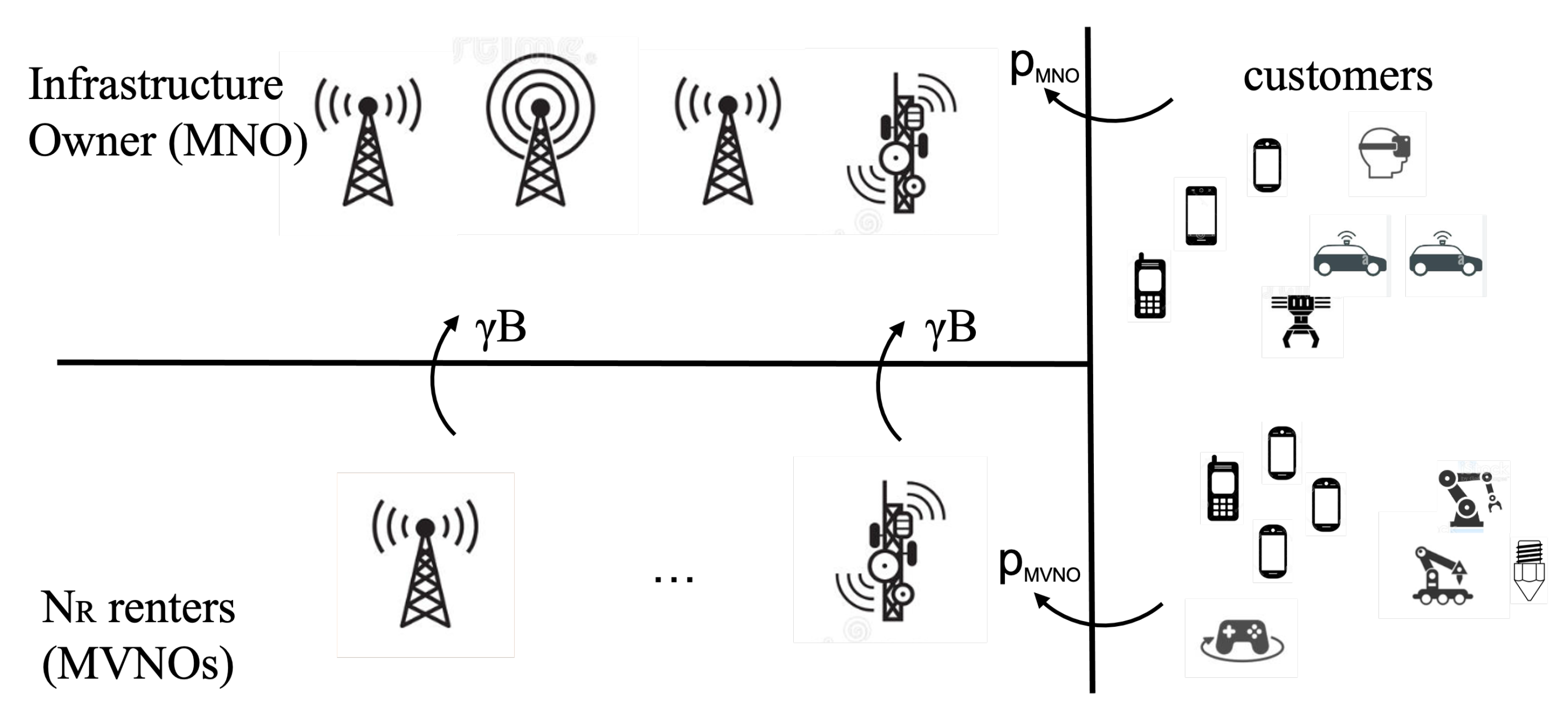
3. The 5G Infrastructure: Network Operators, Pricing Plans, and Customer Preferences
- The radio access network (RAN), which is responsible for connecting devices to the 5G network and providing wireless communication;
- The core network, which provides the routing and switching functionality needed to connect devices to the internet and other networks;
- The transport network, which provides the physical infrastructure needed to connect the RAN and core network;
- The management and orchestration layer, which is responsible for configuring and controlling the network elements and services;
- The security layer, which provides end-to-end security for the network and its users.
- Pay-as-you-go plans, which allow customers to pay for only the minutes, texts, and data that they use; this plan can be a good option for customers who do not use their phone frequently or who want to avoid the commitment of a long-term contract;
- Prepaid plans, which require customers to pay in advance for a set amount of minutes, texts, and data and to add more credit to continue using the service when they have used up their prepaid balance;
- Postpaid plans, which allow customers to use the service and pay for it at the end of the month and can be a good option for customers who use their phone frequently and want the convenience of not having to constantly add credit to their account;
- Monthly plans, which typically offer a set amount of minutes, texts, and data for a fixed monthly fee and can be a good option for customers who use their phone frequently and want a predictable monthly bill;
- Family plans, which allow multiple people on the same account to share minutes, texts, and data, and can be a good option for families or groups of friends who want to save money on their mobile service.
- Wholesale rate on a per-minute, per-text, or per-data-unit basis; this rate is typically lower than the retail rate that MNOs charge their own customers;
- Flat rate for a set amount of minutes, texts, and data, which can be a good option for MVNOs that want a predictable monthly bill and want to offer fixed plans to their customers;
- Reseller agreements, where the MVNOs resell the MNOs service with a markup;
- Revenue sharing agreements, where the MVNOs pay a percentage of their revenue to the MNOs in exchange for network access.
- Network coverage and reliability, because customers may prefer an operator with better network coverage and reliability; a good network coverage allows the customers to have seamless access to services and to be able to connect in more places;
- Quality of service, because customers may prefer an operator that offers a higher quality of service, such as faster internet speeds or better customer service;
- Brand reputation, because customers may prefer an operator that has a good reputation and a long history of providing quality service;
- Offered services, because customers may prefer an operator that offers additional services such as international roaming plans, more flexible plans, more family plans, more roaming plans, and more data plans;
- Device availability, because customers may prefer an operator that offers the latest and most desirable devices for purchase or on contract;
- Bundles and discounts, because customers may prefer an operator that offers bundled services such as TV, internet, and home phone services or offers discounts for combining services;
- Loyalty programs, because customers may prefer an operator that rewards loyal customers with discounts or other benefits.
4. Operators’ Costs, Revenues, and Profits
4.1. Cost Models
- The CAPEXs of the MNO are linearly related to the bandwidth;
- OPEXs are proportional to the CAPEXs;
- The CAPEXs and OPEXs of MVNOs are a fraction of those pertaining to the MNO;
- Renting is priced linearly in the bandwidth so that the renting fee is expressed per unit bandwidth.
4.2. The Demand Function
- when ;
- when all the renters give their service for free, i.e., , , so that .
4.3. Customers
4.4. Profits
5. The Owner–Renter Game
- Owner;
- Renters;
- Regulator.
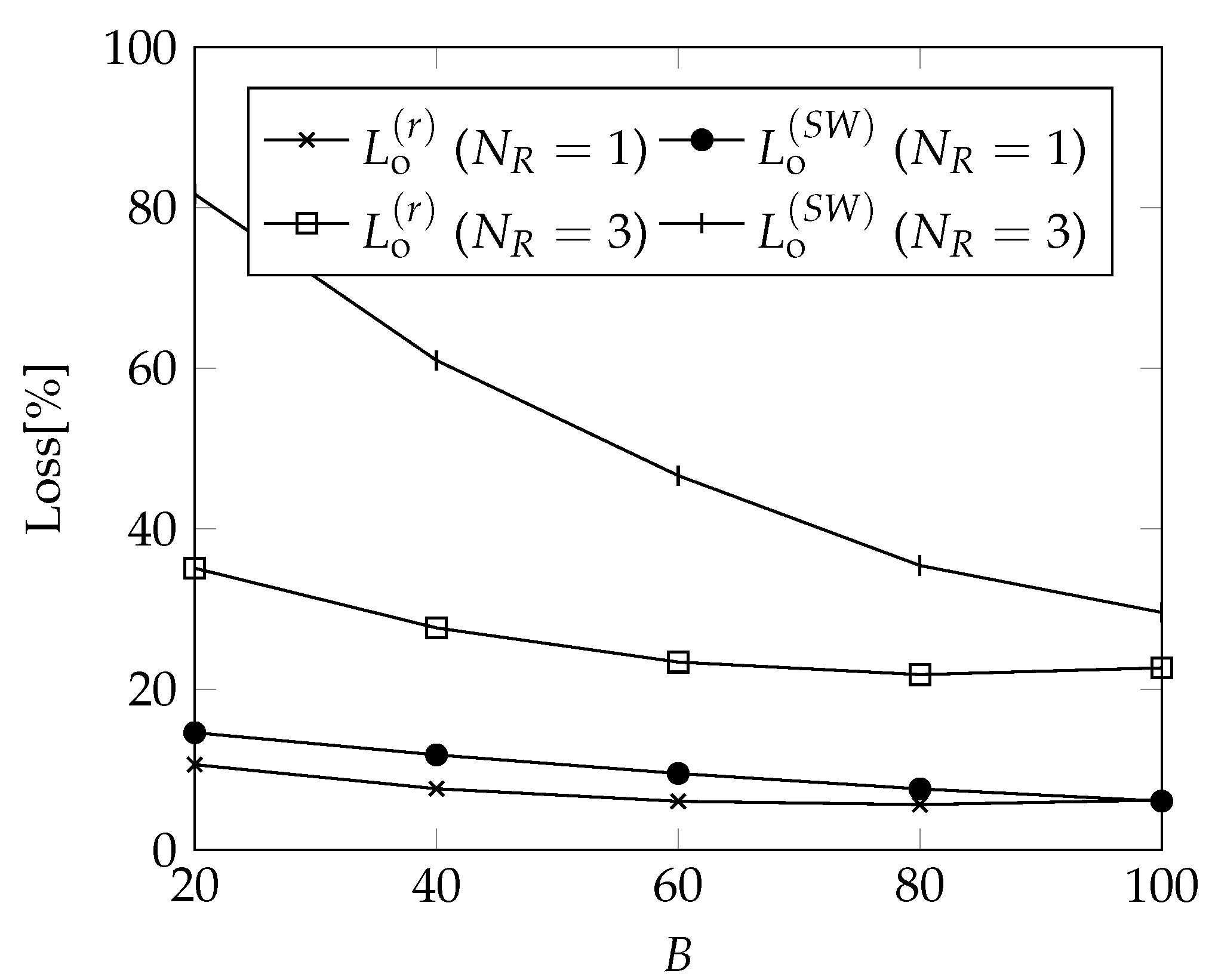
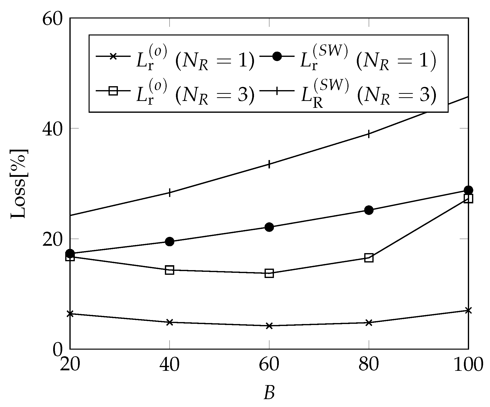
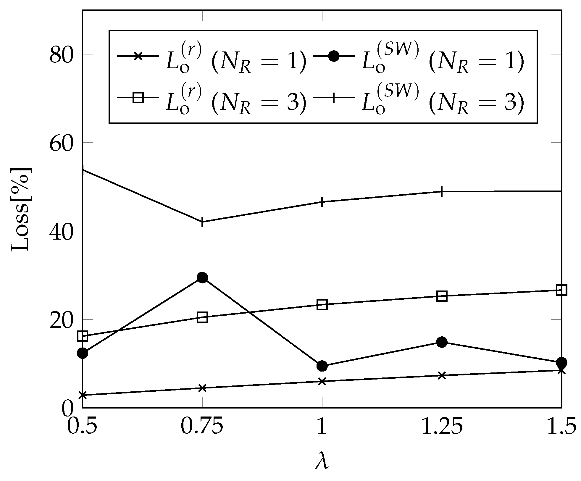
6. Results
7. Conclusions
Author Contributions
Funding
Data Availability Statement
Conflicts of Interest
Appendix A. Glossary of Terms

| Symbol | Definition/Description |
|---|---|
| n | number of potential customers |
| overall number of customers | |
| number of customers joining the operator x | |
| number of renters | |
| number of customers of the MNO | |
| number of customers of the generic MVNO | |
| CMNO | cost function for the MNO |
| cost function for the i-th MNVO | |
| price imposed by the MNO | |
| price imposed by the i-thMVNO | |
| average price imposed by the MVNO | |
| average price | |
| profit of MNO | |
| profit of the generic MVNO | |
| ratio of the number of actual customers to the number of potential customers | |
| quasi-elasticity of the demand function with respect to the average price | |
| price offered by operator h under price-setting scenario k ** | |
| profit of operator h under price-setting scenario k ** | |
| profit loss of operator h under price-setting scenario k ** | |
| SW | social welfare |
| zero-consumption fee in the linear cost model | |
| m | marginal cost of bandwidth |
| B | bandwidth |
| OPEX/CAPEX ratio | |
| CAPEX fraction borne by the i-th MVNO | |
| OPEX fraction borne by the i-th MVNO | |
| renting fee for each bandwidth unit | |
| z | value of the quasi-elasticity of the demand function with respect to the average price |
| stickiness factor |
Appendix B. Maximization of Profits
References
- Gohil, A.; Modi, H.; Patel, S.K. 5G technology of mobile communication: A survey. In Proceedings of the 2013 International Conference on Intelligent Systems and Signal Processing (ISSP), Vallabh Vidyanagar, India, 1–2 March 2013; IEEE: New York, NY, USA, 2013; pp. 288–292. [Google Scholar]
- Dogra, A.; Jha, R.K.; Jain, S. A survey on beyond 5G network with the advent of 6G: Architecture and emerging technologies. IEEE Access 2020, 9, 67512–67547. [Google Scholar] [CrossRef]
- García-Pineda, M.; Felici-Castell, S.; Segura-García, J. Adaptive SDN-based architecture using QoE metrics in live video streaming on Cloud Mobile Media. In Proceedings of the 2017 Fourth International Conference on Software Defined Systems (SDS), Valencia, Spain, 8–11 May 2017; IEEE: New York, NY, USA, 2017; pp. 100–105. [Google Scholar]
- Segura-Garcia, J.; Felici-Castell, S.; Garcia-Pineda, M. Performance evaluation of different techniques to estimate subjective quality in live video streaming applications over LTE-Advance mobile networks. J. Netw. Comput. Appl. 2018, 107, 22–37. [Google Scholar] [CrossRef]
- Oughton, E.J.; Katsaros, K.; Entezami, F.; Kaleshi, D.; Crowcroft, J. An open-source techno-economic assessment framework for 5G deployment. IEEE Access 2019, 7, 155930–155940. [Google Scholar] [CrossRef]
- Naldi, M.; Pacifici, A.; Tagliacozzo, A.; Nicosia, G. Build or Merge: Locational Decisions in Mobile Access Networks. In Proceedings of the 2018 UKSim-AMSS 20th International Conference on Computer Modelling and Simulation (UKSim), Cambridge, UK, 27–29 March 2018; IEEE: New York, NY, USA, 2018; pp. 133–138. [Google Scholar]
- Village, J.; Worrall, K.; Crawford, D. 3G shared infrastructure. In Proceedings of the Third International Conference on 3G Mobile Communication Technologies, London, UK, 8–10 May 2002; IET: London, UK, 2002; pp. 10–16. [Google Scholar]
- Samdanis, K.; Costa-Perez, X.; Sciancalepore, V. From network sharing to multi-tenancy: The 5G network slice broker. IEEE Commun. Mag. 2016, 54, 32–39. [Google Scholar] [CrossRef] [Green Version]
- Afraz, N.; Slyne, F.; Gill, H.; Ruffini, M. Evolution of access network sharing and its role in 5G networks. Appl. Sci. 2019, 9, 4566. [Google Scholar] [CrossRef] [Green Version]
- Sciancalepore, V.; Samdanis, K.; Costa-Perez, X.; Bega, D.; Gramaglia, M.; Banchs, A. Mobile traffic forecasting for maximizing 5G network slicing resource utilization. In Proceedings of the IEEE INFOCOM 2017-IEEE Conference on Computer Communications, Atlanta, GA, USA, 1–4 May 2017; IEEE: New York, NY, USA, 2017; pp. 1–9. [Google Scholar]
- Larsen, K. Network sharing fundamentals. Technol. Bus. 2012, 7. [Google Scholar]
- Smura, T.; Kiiski, A.; Hämmäinen, H. Virtual operators in the mobile industry: A techno-economic analysis. NETNOMICS Econ. Res. Electron. Netw. 2007, 8, 25–48. [Google Scholar] [CrossRef]
- Varoutas, D.; Katsianis, D.; Sphicopoulos, T.; Stordahl, K.; Welling, I. On the economics of 3G mobile virtual network operators (MVNOs). Wirel. Pers. Commun. 2006, 36, 129–142. [Google Scholar] [CrossRef]
- Luong, N.C.; Wang, P.; Niyato, D.; Liang, Y.C.; Han, Z.; Hou, F. Applications of economic and pricing models for resource management in 5G wireless networks: A survey. IEEE Commun. Surv. Tutorials 2018, 21, 3298–3339. [Google Scholar] [CrossRef] [Green Version]
- Guijarro, L.; Pla, V.; Vidal, J.R.; Naldi, M. Maximum-profit two-sided pricing in service platforms based on wireless sensor networks. IEEE Wirel. Commun. Lett. 2015, 5, 8–11. [Google Scholar] [CrossRef] [Green Version]
- Guijarro, L.; Vidal, J.R.; Pla, V.; Naldi, M. Economic analysis of a multi-sided platform for sensor-based services in the internet of things. Sensors 2019, 19, 373. [Google Scholar] [CrossRef] [Green Version]
- Guijarro, L.; Pla, V.; Vidal, J.R.; Naldi, M. Competition in data-based service provision: Nash equilibrium characterization. Future Gener. Comput. Syst. 2019, 96, 35–50. [Google Scholar] [CrossRef]
- Sapavath, N.N.; Rawat, D.B. Wireless virtualization architecture: Wireless networking for Internet of Things. IEEE Internet Things J. 2019, 7, 5946–5953. [Google Scholar] [CrossRef]
- Chang, Z.; Zhu, K.; Zhou, Z.; Ristaniemi, T. Service provisioning with multiple service providers in 5G ultra-dense small cell networks. In Proceedings of the 2015 IEEE 26th Annual International Symposium on Personal, Indoor, and Mobile Radio Communications (PIMRC), Hong Kong, China, 30 August–2 September 2015; IEEE: New York, NY, USA, 2015; pp. 1895–1900. [Google Scholar]
- Zhao, H.; Deng, S.; Liu, Z.; Xiang, Z.; Yin, J.; Dustdar, S.; Zomaya, A.Y. Dpos: Decentralized, privacy-preserving, and low-complexity online slicing for multi-tenant networks. IEEE Trans. Mob. Comput. 2021, 21, 4296–4309. [Google Scholar] [CrossRef]
- Assila, B.; Kobbane, A.; Elmachkour, M.; El Koutbi, M. A dynamic stackelberg-cournot game for competitive content caching in 5G networks. In Proceedings of the 2017 International Conference on Wireless Networks and Mobile Communications (WINCOM), Rabat, Morocco, 1–4 November 2017; IEEE: New York, NY, USA, 2017; pp. 1–6. [Google Scholar]
- Zhang, W.; Li, X.; Zhao, L.; Yang, X. Competition of duopoly MVNOs for IoT applications through wireless network virtualization. Wirel. Commun. Mob. Comput. 2020, 2020, 8880307. [Google Scholar] [CrossRef]
- Gang, J.; Friderikos, V. Optimal resource sharing in multi-tenant 5G networks. In Proceedings of the 2018 IEEE Wireless Communications and Networking Conference (WCNC), Barcelona, Spain, 15–18 April 2018; IEEE: New York, NY, USA, 2018; pp. 1–6. [Google Scholar]
- Akgul, O.U.; Malanchini, I.; Capone, A. Slice-Aware Capacity Expansion Strategies in Multi-Tenant Networks. In Proceedings of the 2019 IEEE Global Communications Conference (GLOBECOM), Waikoloa, HI, USA, 9–13 December 2019; IEEE: New York, NY, USA, 2019; pp. 1–6. [Google Scholar]
- Gedel, I.; Nwulu, N. Infrastructure Sharing for 5G Deployment: A Techno-Economic Analysis; International Association of Online Engineering: Vienna, Austria, 2021. [Google Scholar]
- Landertshamer, O.; Benseny, J.; Hämmäinen, H.; Wainio, P. Cost model for a 5G smart light pole network. In Proceedings of the 2019 CTTE-FITCE: Smart Cities & Information and Communication Technology (CTTE-FITCE), Ghent, Belgium, 25–27 September 2019; IEEE: New York, NY, USA, 2019; pp. 1–6. [Google Scholar]
- Bugár, G.; Vološin, M.; Maksymyuk, T.; Zausinová, J.; Gazda, V.; Horváth, D.; Gazda, J. Techno-economic framework for dynamic operator selection in a multi-tier heterogeneous network. Ad. Hoc. Netw. 2020, 97, 102007. [Google Scholar] [CrossRef]
- Sacoto-Cabrera, E.J.; Guijarro, L.; Vidal, J.R.; Pla, V. Economic feasibility of virtual operators in 5G via network slicing. Future Gener. Comput. Syst. 2020, 109, 172–187. [Google Scholar] [CrossRef]
- Hou, J.; Sun, L.; Shu, T.; Xiao, Y.; Krunz, M. Economics of strategic network infrastructure sharing: A backup reservation approach. IEEE/ACM Trans. Netw. 2020, 29, 665–680. [Google Scholar] [CrossRef]
- Khamse-Ashari, J.; Senarath, G.; Bor-Yaliniz, I.; Yanikomeroglu, H. An agile and distributed mechanism for inter-domain network slicing in next-generation mobile networks. IEEE Trans. Mob. Comput. 2021, 10, 3486–3501. [Google Scholar] [CrossRef]
- Barua, B.; Matinmikko-Blue, M.; Latva-aho, M. On emerging contractual relationships for local 5G micro operator networks. In Proceedings of the 2019 16th International Symposium on Wireless Communication Systems (ISWCS), Oulu, Finland, 27–30 August 2019; IEEE: New York, NY, USA, 2019; pp. 703–708. [Google Scholar]
- Qian, B.; Zhou, H.; Ma, T.; Yu, K.; Yu, Q.; Shen, X. Multi-operator spectrum sharing for massive IoT coexisting in 5G/B5G wireless networks. IEEE J. Sel. Areas Commun. 2020, 39, 881–895. [Google Scholar] [CrossRef]
- Flamini, M.; Naldi, M. Cournot equilibrium in an owner-renter model for 5G networks under flat-rate pricing. In Proceedings of the 2020 43rd International Conference on Telecommunications and Signal Processing (TSP), Milan, Italy, 7–9 July 2020; IEEE: New York, NY, USA, 2020; pp. 158–161. [Google Scholar]
- 3GPP TS 38.300 ETSI Technical Specification: NR and NG-RAN Overall Description; Version 16.2.0; 3GPP: Sophia Antipolis, France, 2020.
- 3GPP TS 23.501 ETSI Technical Specification: System Architecture for the 5G System; Version 15.2.0; 3GPP: Sophia Antipolis, France, 2018.
- Khalifa, N.B.; Benhamiche, A.; Simonian, A.; Bouillon, M. Profit and strategic analysis for MNO-MVNO partnership. In Proceedings of the 2018 IFIP Networking Conference (IFIP Networking) and Workshops, Zurich, Switzerland, 14–16 May 2018; IEEE: New York, NY, USA, 2018; pp. 325–333. [Google Scholar]
- Debbah, M.; Echabbi, L.; Hamlaoui, C. Market share analysis between MNO and MVNO under brand appeal based segmentation. In Proceedings of the 2012 6th International Conference on Network Games, Control and Optimization (NetGCooP), Avignon, France, 28–30 November 2012; IEEE: New York, NY, USA, 2012; pp. 9–16. [Google Scholar]
- Knoll, T.M. A combined CAPEX and OPEX cost model for LTE networks. In Proceedings of the 2014 16th International Telecommunications Network Strategy and Planning Symposium (Networks), Funchal, Portugal, 17–19 September 2014; IEEE: New York, NY, USA, 2014; pp. 1–6. [Google Scholar]
- Rahman, M.; Despins, C.; Affes, S. Analysis of CAPEX and OPEX benefits of wireless access virtualization. In Proceedings of the 2013 IEEE International Conference on Communications Workshops (ICC), Budapest, Hungary, 9–13 June 2013; IEEE: New York, NY, USA, 2013; pp. 436–440. [Google Scholar]
- Youssef, M.; Al Zahr, S.; Gagnaire, M. Translucent network design from a CapEx/OpEx perspective. Photonic Netw. Commun. 2011, 22, 85–97. [Google Scholar] [CrossRef]
- Gruber, C.G. Capex and opex in aggregation and core networks. In 2009 Conference on Optical Fiber Communication-Incudes Post Deadline Papers; IEEE: New York, NY, USA, 2009; pp. 1–3. [Google Scholar]
- Jarray, A.; Jaumard, B.; Houle, A.C. CAPEX/OPEX effective optical wide area network design. Telecommun. Syst. 2012, 49, 329–344. [Google Scholar] [CrossRef]
- Hardin, A.; Ergas, H.; Small, J. Economic depreciation in telecommunications cost models. In Industry Economics Conference Regulation, Competition and Industry Structure; NECG: Claremont, CA, USA, 1999; pp. 12–13. [Google Scholar]
- Nikolikj, V.; Janevski, T. Cost-effectiveness assessment of 5G systems with cooperative radio resource sharing. Telfor J. 2015, 7, 68–73. [Google Scholar] [CrossRef] [Green Version]
- Verbrugge, S.; Colle, D.; Pickavet, M.; Demeester, P.; Pasqualini, S.; Iselt, A.; Kirstädter, A.; Hülsermann, R.; Westphal, F.J.; Jäger, M. Methodology and input availability parameters for calculating OpEx and CapEx costs for realistic network scenarios. J. Opt. Netw. 2006, 5, 509–520. [Google Scholar] [CrossRef]
- Pei, J.; Hong, P.; Xue, K.; Li, D. Efficiently embedding service function chains with dynamic virtual network function placement in geo-distributed cloud system. IEEE Trans. Parallel Distrib. Syst. 2018, 30, 2179–2192. [Google Scholar] [CrossRef]
- Reyes, R.R.; Sultana, S.; Pai, V.V.; Bauschert, T. Analysis and evaluation of CAPEX and OPEX in intra-data centre network architectures. In Proceedings of the 2019 IEEE Latin-American Conference on Communications (LATINCOM), Salvador, Brazil, 11–13 November 2019; IEEE: New York, NY, USA, 2019; pp. 1–6. [Google Scholar]
- Talluri, K.T.; Van Ryzin, G.; Van Ryzin, G. The Theory and Practice of Revenue Management; Springer: Berlin/Heidelberg, Germany, 2004; Volume 1. [Google Scholar]
- Postigo-Boix, M.; Melus-Moreno, J.L. A proposal for pricing substitute guaranteed services. IEEE Commun. Lett. 2010, 15, 100–102. [Google Scholar] [CrossRef]
- Postigo-Boix, M.; Melús-Moreno, J.L. Generating demand functions for data plans from mobile network operators based on users’ profiles. J. Netw. Syst. Manag. 2018, 26, 904–928. [Google Scholar] [CrossRef] [Green Version]
- Shankar, A.; Morya, K.K. Pricing of Mobile Telephony Services in India. Int. J. Emerg. Technol. 2020, 11, 120–134. [Google Scholar]
- Turel, O.; Serenko, A. Satisfaction with mobile services in Canada: An empirical investigation. Telecommun. Policy 2006, 30, 314–331. [Google Scholar] [CrossRef]
- Choi, J.; Seol, H.; Lee, S.; Cho, H.; Park, Y. Customer satisfaction factors of mobile commerce in Korea. Internet Res. 2008, 18, 313–335. [Google Scholar] [CrossRef]
- Gerpott, T.J.; Rams, W.; Schindler, A. Customer retention, loyalty, and satisfaction in the German mobile cellular telecommunications market. Telecommun. Policy 2001, 25, 249–269. [Google Scholar] [CrossRef]
- Calvo-Porral, C.; Lévy-Mangin, J.P. Switching behavior and customer satisfaction in mobile services: Analyzing virtual and traditional operators. Comput. Hum. Behav. 2015, 49, 532–540. [Google Scholar] [CrossRef]
- Ida, T.; Sakahira, K. Broadband migration and lock-in effects: Mixed logit model analysis of Japan’s high-speed Internet access services. Telecommun. Policy 2008, 32, 615–625. [Google Scholar] [CrossRef]
- Czajkowski, M.; Sobolewski, M. How much do switching costs and local network effects contribute to consumer lock-in in mobile telephony? Telecommun. Policy 2016, 40, 855–869. [Google Scholar] [CrossRef]
- Calvo-Porral, C.; Faíña-Medín, A.; Nieto-Mengotti, M. Satisfaction and switching intention in mobile services: Comparing lock-in and free contracts in the Spanish market. Telemat. Inform. 2017, 34, 717–729. [Google Scholar] [CrossRef]
- Lu, N.; Lin, H.; Lu, J.; Zhang, G. A customer churn prediction model in telecom industry using boosting. IEEE Trans. Ind. Informatics 2012, 10, 1659–1665. [Google Scholar] [CrossRef]
- Mahajan, V.; Misra, R.; Mahajan, R. Review on factors affecting customer churn in telecom sector. Int. J. Data Anal. Tech. Strateg. 2017, 9, 122–144. [Google Scholar] [CrossRef]
- Dasgupta, K.; Singh, R.; Viswanathan, B.; Chakraborty, D.; Mukherjea, S.; Nanavati, A.A.; Joshi, A. Social ties and their relevance to churn in mobile telecom networks. In Proceedings of the 11th International Conference on Extending Database Technology: Advances in Database Technology, Nantes, France, 25–29 March 2008; pp. 668–677. [Google Scholar]
- Sherrington, S. 2020 in Review 5G Networks, Spectrum & Devices; Technical Report; Global mobile Suppliers Association: Farnham, UK, 2020. [Google Scholar]
- Meddour, D.E.; Rasheed, T.; Gourhant, Y. On the role of infrastructure sharing for mobile network operators in emerging markets. Comput. Netw. 2011, 55, 1576–1591. [Google Scholar] [CrossRef] [Green Version]
- Dennis, J.E., Jr.; Schnabel, R.B. Numerical Methods for Unconstrained Optimization and Nonlinear Equations; SIAM: Philadelphia, PA, USA, 1996. [Google Scholar]


| Parameter | Value |
|---|---|
| 11.5 | |
| m | 0.0003 |
| B | 60 |
| 0.5 | |
| 0.1 | |
| 0.5 | |
| 0.7 | |
| z | 0.0005 |
| 0.5 |
| monopoly | 116,439 | NA | NA | NA | NA | NA |
| 63,083 | 51,899 | 59,276 | 54,194 | 57,088 | 42,208 | |
| 38,564 | 23,655 | 29,548 | 27,424 | 20,591 | 27,350 |
Disclaimer/Publisher’s Note: The statements, opinions and data contained in all publications are solely those of the individual author(s) and contributor(s) and not of MDPI and/or the editor(s). MDPI and/or the editor(s) disclaim responsibility for any injury to people or property resulting from any ideas, methods, instructions or products referred to in the content. |
© 2023 by the authors. Licensee MDPI, Basel, Switzerland. This article is an open access article distributed under the terms and conditions of the Creative Commons Attribution (CC BY) license (https://creativecommons.org/licenses/by/4.0/).
Share and Cite
Flamini, M.; Naldi, M. Optimal Pricing in a Rented 5G Infrastructure Scenario with Sticky Customers. Future Internet 2023, 15, 82. https://doi.org/10.3390/fi15020082
Flamini M, Naldi M. Optimal Pricing in a Rented 5G Infrastructure Scenario with Sticky Customers. Future Internet. 2023; 15(2):82. https://doi.org/10.3390/fi15020082
Chicago/Turabian StyleFlamini, Marta, and Maurizio Naldi. 2023. "Optimal Pricing in a Rented 5G Infrastructure Scenario with Sticky Customers" Future Internet 15, no. 2: 82. https://doi.org/10.3390/fi15020082