1. Introduction
Due to various climate changes as well as the increasing depletion of resources, conventional energy sources are becoming less important. Photovoltaics, breeze, biomass, as well as other quasi-energy sources are free of the aforementioned issues and hence are set to play a big role in the long term [
1], and investigated the impact of anticipated worldwide warming with the efficiency of PV installations. Renewable radiation is quickly emerging among the most potent sources of power for home, commercial, and commercial applications [
2]. Nonetheless, among the most significant drawbacks of alternative energy sources are their unpredictability. PV plants create various quantities of power depending on solar irradiance and other weather variables [
3]. There could be large differences in electricity production not only between months but as well as between hours and even between minutes [
4]. This would have the possibility to trigger grid load-generation mismatches, making solar photovoltaic prediction critical, especially in systems with significant PV systems [
5]. The penetration of renewable into the electrical grid is becoming increasingly important, but it is also posing tough possibilities for electricians and academics. Photovoltaic power’s irregular and unpredictable nature complicates network administration and contributes to the difficulty of balancing electrical energy supply and demand [
6]. Regarding electrical operators, striking a balance across power systems has become a major task. Further challenges that develop as a result of solar energy’s unpredictable nature include voltage swings, poor power quality, as well as inertness. The primary technological issues electricity administrators face when combining alternative fuels with the power grid are variability, unpredictability, and parallel activities [
7]. As more than just a result, reliable predicting of Photovoltaic solar output is essential for proper microgrids [
8]. Photovoltaic prediction is necessary for scheduling, estimating stocks, managing produced electricity supply, improving power grid functioning, lowering costs of generated electrical energy, and managing congestion, and because of the aforementioned power issues currently, solar power forecast has become more crucial in prevalence among solar grid growth [
9]. To manage energy variance, research recommends combining storage systems with clean energy forecasts.
Storage technologies capture additional power, moderate oscillations, and keep the electricity flowing [
10]. This whole article will address and relate various prediction methods for estimating PV output power in two directions: (i) straightforward prediction, which either forecasts additional power utilizing chronological PV energy data, and (ii) indirect predicting, which also utilizes solar insulation accurate forecasts, as well as other weather parameters that directly impact solar PV manufacturing [
11]. Related to physical hypotheses about the air, a variety of methodologies enabling PV power prediction have indeed been presented. A good number of the extensively worn physiological model is the NWP [
12]. The weather data forecast model is technologically complicated and challenging due to the atmosphere’s fluctuation and unexpectedness [
13]. Machine learning approaches are becoming more prominent as the area of computer engineering expands as well as its capacity to interact with non-linearity improves [
14]. One such study analyses, assesses, and then contrasts several types of panel irradiance estimate algorithms and PV-performing metrics in the domain of PV power predictions [
15], in addition to the immediate and oblique PV power forecasting utilizing ML approaches. There are two types of solar power PV panels. One is on a large scale, i.e., on account of its power capacity, in megawatts scale, being installed over a wide area [
16]. Most of this electricity is used by the companies that installed them or sold them to power companies. Second, small power capacity solar panels are installed on roofs of houses, hotels, and commercial establishments for personal use [
17]. In this, it is connected to the electrical connection of the power company and operates; On the other hand, there are two types of independent operation without connection to the mains. There are many difficulties operating without a proper electrical connection [
18]. First, it needs a battery. Battery maintenance costs are also a problem. When electricity is produced more than we need, the electricity from sunlight goes to waste when the battery is full of capacity [
19]. Apart from this, 15 to 20 percent of energy is wasted due to the storage and reuse of electricity in batteries.
Solar panels or photovoltaic systems using panels (SPV panels) are placed on rooftops or solar farms arranged so that solar radiation falls on the solar photovoltaic panels to facilitate the reaction of converting sunlight into electricity [
20]. A solar photovoltaic system converts solar energy into electrical energy. A battery converts chemical energy into electrical energy, an automobile engine converts chemical energy into mechanical energy, or an electric motor (in an electric vehicle, EV) converts electrical into mechanical energy [
21]. An SPV cell converts solar energy into electrical energy. A solar cell does not use the sun’s heat to generate electricity, but light rays interact with semiconductor materials to generate electricity. This current flows from the semiconductor to the output leads. These leads are connected to batteries or grids through some electronic circuits and inverters to control and generate alternating currents [
22]. Solar energy is used for a home, industrial unit, or small community. A disadvantage of this system is that when the power goes out, the system also shuts down. It is for safety reasons, as grid-tied inverters should automatically disconnect when they do not sense the grid. It means that during a blackout or emergency, It cannot supply power and store energy for later use [
23,
24]. The following are the key contributions of the manuscript:
The main contribution of this research is to develop autonomous forecasting models with a larger range of features that accurately recognizes occurrences. Here, an AUTO-encoded-based Neural Network (AUTO-NN) forecast model combines a Restricted Boltzmann Machines (RBM) for image retrieval and a Back Propagation Neural Network (BPNN) for component categorization.
The organization of this article is given as the following
Section 1 illustrates the locale of photovoltaic plants, energy generation, and the role of deep learning in the energy prediction field. In
Section 2, the literature on energy prediction is reviewed.
Section 3 explains the projected energy forecasting process by means of constructing an arrangement. In
Section 4, the investigational study is specified among graphs by evaluating three customary techniques. Finally,
Section 5 presents the conclusion and future research direction.
2. Related Works
Sittón-Candanedo et al. [
25] expressed a Review on Edge Computing in Smart Energy using a Systematic Mapping Study. Renewable energy is critical to the long-term viability of energy and the environment. The highly recommended energy projects in Malaysia found that the most useful elements in fuel consumption are modern energy availability, particularly for low individuals as well as remote regions. Kim, T et al. [
26] discussed the analysis and Impact Evaluation of Missing Data Imputation in Day-ahead PV Generation Forecasting. Bayesian network analysis was used to predict the most electricity main refrigerants. A construction dataset with good energy efficiency was used to train the Bayesian network approach. The learning algorithm was used to determine which buildings’ major refrigerants should be installed. D. Hartono et al. [
27] expressed Modern energy consumption assessment for accessibility and affordability. These observations backed up the overall validity of data-driven architecture. The data-driven methodologies for monitoring energy and costs were examined. Their findings indicated that data-driven techniques, including load projections, energy consumption profiles, and retrofit solutions, have indeed been widely utilized in the energy domain.
Z. Tian et al. [
28] discussed an application of the Bayesian Network approach for selecting energy-efficient HVAC systems. The ANNs concept was shown to be the majority accepted in applications ranging from force forecast to retrofit resolution, according to their research. Because of their ease of development, SVM models were frequently utilized for extensive construction liveliness analyses. W. Tian et al. [
29] expressed an identifying informative energy data in Bayesian calibration of building energy models. Here the authors looked studied information ways for estimating energy use in buildings. This research looked into the predictive ranges, pre-processing stage methodologies, machine learning classification algorithms, and assessment key metrics. K. Amasyali et al. [
30] provide a review of data-driven building energy consumption prediction studies. There have been two types of building structures of prediction points of view: industrial and residential structures; five different concentrations have been used: sub-hourly, regular, weekly, quarterly, and annually. In terms of information size, the majority of the research examined used a one-month interval between individual samples.
N. Somu et al. [
31] discussed a deep learning framework for building energy consumption forecasts To model urban energy consumption in buildings. They introduced a novel infrastructure machine learning method (ResNet). Researchers employed the benchmark energy modeling model to create the needed periodical collected information for every property, which was then used to train the data-driven model. M. Najafzadeh et al. [
32] expressed a Riprap incipient motion for overtopping flows with machine learning models. Furthermore, to model the ‘hidden’ effects of the urban environment, which are not represented in the actual building computation, a deep residual program was built. Researchers developed a hybrid methodology for simulating power usage in various spatiotemporal qualities by disciplines’ expertise with neural networks. S. Seyedzadeh et al. [
33] discussed Tuning machine learning models for the prediction of building energy loads. Unfortunately, extracting the thickness of hidden units in ResNet can understand the relationships among demand in nearby buildings are time-consuming, and obtaining data and information beginning a physics-induced form was taking more time.
Luis Hernández et al. [
34] provided an introduction to a multi-agent system architecture for smart grid management and forecasting of energy demand in virtual power plants. The SVM, MARS, and RF models were used to forecast the approaches dens metric Froude score at the impending movement of riprap particles, which could also prevent streams against degradation. N. R. Canada et al. [
35] provided High-resolution solar radiation datasets. The performance of the machine learning model that can predict indoor thermal comfort in buildings was assessed. Autoencoders, gradient boosting analysis, Gaussian procedure (GP), randomized forest, and gradient boosted regression trees were among the Machine learning they looked into it. It had superior performance in terms of the RMSE (root-mean-square error) ratio, according to their findings. P. Shamsi et al. [
36] express Preemptive control: A paradigm in supporting high renewable penetration levels. Researchers also concluded that with complicated datasets, the ANNs approach had been the perfect suit. The ANNs paradigm has a faster computational effort than the other ML mode studied throughout the investigation.
J. Logeshwaran et al. [
37] discuss the role of integrated structured cabling systems for reliable bandwidth optimization in the high-speed communication network. Through the assessment of the current state of knowledge introduced above, a genuine need disparity in the existing research. Shisheng Fu et al. [
38] discussed Automatic RF-EMF Radiated Immunity Test System for Electricity Meters in Power Monitoring Sensor Networks. It can be identified that improving a precise long-term hourly prediction for the period consumed energy in the presence of a wide variety of electricity consumers without experiencing a significant drop in forecasting accuracy, which typically occurs after the first two weeks.
Balasubramaniam S et al. [
39] expressed Fractional Feedback Political Optimizer with Prioritization-Based Charge Scheduling in Cloud-Assisted Electric Vehicular Network. Energy can be transferred to a particular place or element, but it is something that cannot be created or destroyed. Energy, absorbed in the various forms it can take, has the potential to be used in a variety of ways. Focusing on energy and every variation of each model would be too broad and complex. Visser L et al. [
40] discussed Operational day-ahead solar power forecasting for aggregated PV systems with a varied spatial distribution. Some of the main sources of global warming are derived from thermal processes due to the exchange reaction of CO
2. The transfer of CO
2 from energy conversion is essentially non-existent.
Tamoor M et al. [
41] expressed the Designing and energy estimation of photovoltaic energy generation systems and prediction of plant performance. Conversion of thermal energy from other forms of energy can be given with high efficiency. Between non-convertible resources or thermal energy, they can be generated with high levels of efficiency, although a certain amount of energy is always wasted in a thermal way, which is similar to friction and process. Khan W et al. [
42] discussed Improved solar photovoltaic energy generation forecast using a deep learning-based ensemble stacking approach. When the minimum approximation point is reached, the process is reversed to go in the opposite direction. It is further increased and converts potential energy into kinetic energy. The process has maximum efficiency as this environment is not practical. Li P et al. [
43] expressed the Effect of the temperature difference between land and lake on photovoltaic power generation. It should be noted that heat energy is specific because it cannot be converted into other energy. It is only possible to use the variation in density that has thermal energy to perform the work, and the efficiency of this variation is less than one hundred percent.
Ren Y et al. [
44] discussed the Optimal design of hydro-wind-PV multi-energy complementary systems considering smooth power output. Thermal energy represents a peculiarly disordered or chaotic energy that is distributed without a particular continuity in the multitude of situations available to the group of particles that make up the systematic mechanism. Rodríguez F et al. [
45] expressed Forecasting intra-hour solar photovoltaic energy by assembling wavelet-based time-frequency analysis with deep learning neural networks. Every type of PV equipment requires energy to operate. All matter that alters or produces changes in its environment contains energy. In all kinds of activities undertaken, energy is of utmost importance. Gao X et al. [
46] discussed Followed The Regularized Leader (FTRL) prediction model-based photovoltaic array reconfiguration for the mitigation of mismatch losses in partial shading conditions. Everything from electrical appliances to electric vehicles requires fuel to run. It combines blocks of chemical energy, which, when placed in contact with a particular hot element, are converted into thermal energy and then into kinetic energy. The comprehensive analysis has shown in the following
Table 1.
The main novelty of this research is to predict the utilization of the PV-based solar-powered and PV-based utility-powered power plants. Hence the method of operating without matching this electrical connection is not popular. Each kilowatt-capacity solar PV system can generate 1500 units of electricity per year. Power generation is likely to vary depending on the amount of solar energy, the angle at which the solar system panels are installed, the weather conditions, the availability of utility power, and the cleanliness of the solar system panels. About six to eight units of electricity are likely to be available daily.
The existing methods of storing and processing naturally generated solar PV energies have some drawbacks. Encoder-based neural network algorithm is designed to solve this problem. The importance of this is that the amount of energy generated can be predicted in advance. Thus the amount of energy generated by Solar PV Plant can be calculated, and design methods can be carried out accordingly. As a result, following this road leads to a dependable, accurate forecasting approach that meets the needs of the contractor, assisting them in achieving long-term economic, business, and management commercial operations.
3. Proposed Model
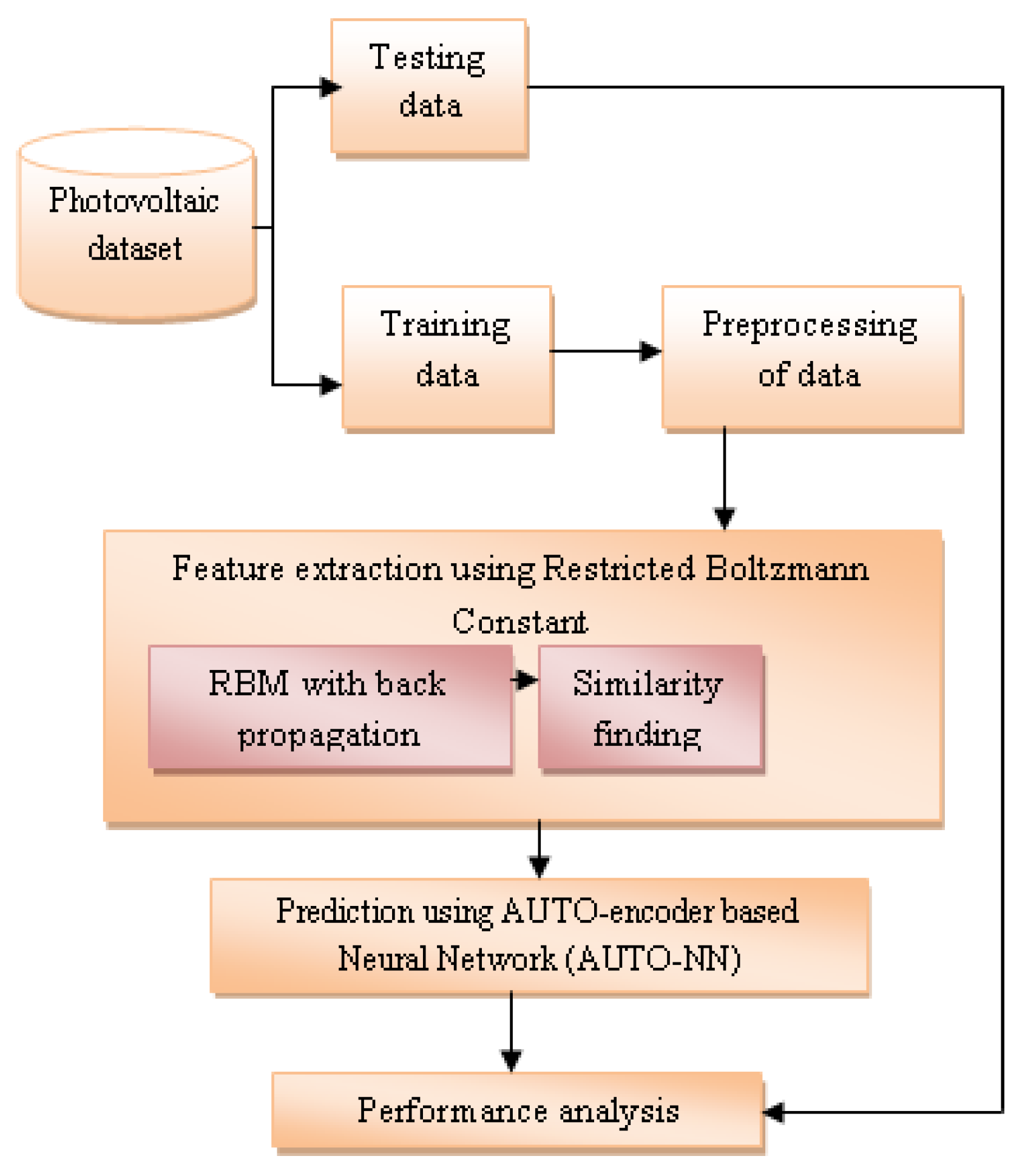
The proposed model was constructed as the listed renewable information is stored in the server. During forecasts, the collected data is loaded into an AUTO-encoder-based Neural Network (AUTO-NN). The photovoltaic dataset is prepared with several inputs based on the first given solar prediction data. Its essential parts can be divided into two categories: testing and training. When the training dataset starts to be managed, its types are first preprocessed. Here, data types of PV models can be collected based on specific attributes and classified into small energy modules. Then feature extraction is done. It is governed by the Boltzmann constant. First, RBM propagation is done. Similarity findings are made from the data obtained through the results. Energy prediction is made based on this data. Finally, a performance comparison is made. It is conducted by comparing test and training data. Based on the results of this, the final results are obtained. Thus the proposed method works.
Figure 1 illustrates the implementation of the energy consumption forecast manner.
Such information was pre-processed utilizing a normalization approach and then used to extract the Restricted Boltzmann Constant automatically. The entire data was divided into two parts: the learning dataset and the testing data, in order to construct computational methods to adjust their strategies. Based on the given data, two types of data set are divided into test data set and training data set. The critical requirements of these data modules become important in correctly segmenting existing data in the proposed method, and by preprocessing the existing data in this proposed method, it is possible to calculate the exact requirements of the input data. These calculations help to accurately predict the amount of energy stored and carry out analyses. Then the data is entered by Restricted Boltzmann Constant, and feature extraction is done. At this point, similarity calculation is done using RBM with backpropagation data. The prediction method based on this data is calculated using the AUTO-encoder-based Neural Network algorithm. Based on these results, the overall system efficiency is calculated.
3.1. Dataset Description
The PV output power dataset (PVOD) is made up of descriptive storage and information records for 10 PV sites using CSV format that might be effortlessly observed in Microsoft Excel Software otherwise Windows. Information is the substance of these documents. The .csv file contains the fundamental data for all PV installations, but the port* file contains extra details. The specifications of weather conditions and in situ observations are contained in the .csv file. Likewise, the number of observations should be large enough for various types of computational modeling training processes to be productive and convenient. PVOD seems to have a cumulative of 271,968 records at the present time and provides numerical weather prediction (NWP) information with a 15-min sampling rate, which is the same as LMD from PV locations. The NWP model that generated the PVOD data is a variant of the Meteorological Studies and Forecasting (WRF) program, especially the Translational edition 4.3.1 techniques to help. ARW is a totally flexible, Iterative quasi model that employs landscape hydrostatic vertical coordinates as well as an Arakawa C-grid staggered spatially singular value decomposition. The model is routinely run thrice during daylight hours with a horizontal lattice frequency of 4 km and 45 landscape (Eta) vertical stages first from level to the top at a pressure of 70 hPa. The simulation is started with 3-hourly, 0.1250.125 global-scale NWP projections from the European Centre for Medium-Range Weather Forecasting (ECMWF), which would be generally observed with one of the universal NWP currently distributed regularly at 12:00 Combined Universal Time (UTC).
3.2. Preprocessing of Training Data
The information is an elevated time series recorded at a resolution of 0.1 kHz. Such elevated data can aid in the prediction of uncommon events and the implementation of preventative measures such as which was before control. The sun irradiation was measured with something such as a LI 200S testing instrument at a wavelength of 1000 Hz and averaged more than 0.01 second quarter. Direct and diffuse irradiance and global tilted brightness, as well as the associated time, are included in the database. Since there are incorrect observations, including such low GHI findings, the information needs to be pre-processed to remove the false reading and night hours, as well as normalize the information. To process raw data, a variety of strategies have been proposed. The most straightforward method is to remove false readings and swap these, including an approximation of prior and subsequent data. The highest constraint is being used to substitute erroneous readings, while linear extrapolation will be used to replace lost data. The material has become clean; however, it contains irrelevant info, including brightness readings that are slightly blurry. It looks for a straight line that connects the two end locations,
xa and
xb. This approach has a number of comparable formulae.
where
α is the interpolation value, which ranges from 0 to 1, and is a number between 0 and 1. Every information is normalized between 0 and 1, as well as the entire posterior distribution of the input parameters is aligned
wherein,
is the input,
= 1 is the number, and
= 0 is the number. One such method assumes that the data before preprocessing contains solely actual values. Adaptive Normalizing is a new data normalization method designed specifically for the non-stationary variables response variables. Its entire data normalizing technique may be broken down into three phases: (i) converting quasi-time series into stable sequences, those results in a set of disjoint shutters (which do not coincide); (ii) anomaly elimination; and (iii) data normalization. The information gathered as a result of these processes is sent into a training algorithm. Examine the normalized series
of a time series
. A fresh sequence
can indeed be described given a set of fixed length
n,
moving average its rolling averages of width, and a sliding window length
,
for all
This series
is broken up into
separate sliding window. As seen, the denominators of all the portions are about the same. This component is critical for maintaining the small–time’ initial trend and ensuring that all values have the same inertia. Every loop has one final output and one input value. Thus the way to build the series R, one must first compute. Afterward, reject the very first values of S if
k > 1, i.e., if the time series order is greater than the number of inputs. For example, if
k == 3, the very first term of series
S should be removed. To begin, we determine the level of modification for each of the training dataset
It really is chosen to be utilized in Adaptive Standardization because it provides the minimum compensation value. The disparity between regression coefficients and residuals of every proportion was employed as our metric, with the primary intent of saving the string R numbers as near to unity as possible. The elimination of outliers from the data sample is a critical process in the data initialization phase, as well as for time series analysis. The fundamental issue with data normalization would be when outliers appear at the outer edges of time–series data, resulting in illogical upper and lower bounds. Because numbers may well be focused on a certain extent of both the normalized range, this will have an impact on the time series statistical data as well as the data normalization accuracy.
3.3. Feature Extraction Using Restricted Boltzmann Machine
The power spectral density E in RBM seems to have the parameterization using weighted vector W as in equation, using variables
v and
h indicating a pair of transparent and concealed variables correspondingly in (6).
The biased factors for transparent and concealed units are indicated by
a and
b, respectively. The probability density
P is calculated using Equation (12) with
v and
h in parameters of
E:
Equation (7) gives the normalizing variable
Z:
Furthermore, the likelihood of v across hidden neurons is provided by Equation (8), which is the combination of the above-mentioned formulae:
Log-likelihood Equation (9) is used to evaluate the variance in training data on the basis of
W:
Here
represent the values expected for the data and distribution model, respectively. The training data is used to calculate weights in the network for document training examples, as shown in Equation (10):
It is feasible to get independent information from that because neurons are not coupled at the concealed or transparent levels. Furthermore, for specified
h and
c, the activating of hidden or visible units is uncorrelated. The conditional property of is provided in Equation (11) for a provided
v:
where
hj ∈ {0,1} and the probability of
hj = 1 is given in Equation (12):
Here the logistic function
σ is specified as in Equation (13):
Likewise, when
vi = 1, the conditional property is estimated by Equation (15),
In practice, unbiased testing is difficult with >, but it could be used to recreate the very first testing of v from h, and thereafter Gibbs sampling will be used for several repetitions. Each component of the concealed and transparent layers is modified in tandem using Gibbs sampling. Finally, by combining the anticipated and modified quantities of h and v, the right selection is calculated with >. Recurrent neural networks can be started with RBM parameters
3.4. Similarity Finding
The frame patterns vary progressively in the incremental changeover, based on development in the
Zij denotes similarity indicators and relationships between pictures. This degree is known as the angular measurement and pertains to the interior production line. The
Zij denotes similarity
zij (sim) could be written as follows:
where, ‘
a’ denotes the anticipated vector based on the most recent observations, while
b denotes the claimed vector based on the most recent data. Let
b = (
xb,
yb,
vb) and
a = (
xb,
yb,
vb) (
xa,
ya,
va). Both of these vectors have three coordinates (
x,
y,
v), with x and y representing xy position information and v representing velocity. In (1),
xb,
yb are the data’s coordinates; vbis is the data’s velocity; and
xa,
ya are the estimated coordinates based on the data obtained well before the current one.
Initially, 3*3 Max-Pooling, as well as a dropout layer with such a parameter of 0.8, was introduced; second, local contrast normalization was employed in the output nodes; and third, during training and testing, the number of iterations was adjusted to 1000. A 3*3 filter with an exponentially quadratic unit activation function was employed in the convolution layer, which was followed by a pooling layer that lowered the dimension of the feature and minimized overfitting. The max-pool layer had a 4*4 filter, the dropout layer had a 0.8 parameter, and the upsampling layer had a 7*7 filter. The proposed Algorithm 1 is shown in the following,
| Algorithm 1: AUTO-encoder-based Neural Network (AUTO-NN) Algorithm |
In: Rx(t), x = 1,2,…n
Out: Out_x(t), out = 1,2,…K and (K + 1)_t of every Out_x(t),
For lay = 0 to lay-1 do
Ki(hi) = Direct(hi) + ki
For every lay do
Initiate {u,v{h<-discrimate (low) and discrimate (low)}
Find the weight (wei)<-0 Disc(sample),{low, high}
For wei (k); k = 1,2…N(iteration)
K > s = {{a1,b1},{a2,b2,}…{an,bn}}
K becomes shrouded layer (sh)
Sh = {1,2,…HH}.g where g = x(t)
Compute fx(t)
Update fx(t) as concealed unit
I(t) = fx(t) < concealed units then
Foundation = testing
else
foundation = concealed units
end if
end for |
The following is a summary of the predefined threshold detector:
Phase 1: If the normalized motion divergence is more than an upper bound thmax, the current frame is chosen as the prospective shot frame .
Phase 2: Finally, we compute the redefined variability as follows:
An equation must be greater than the estimated absolute difference
.
Phase 3: Ultimately, each estimated different segmentation value’s
Zij denbos based on the correlation distance is computed as:
It also has to be larger than a world average .
3.5. Similarity Updating
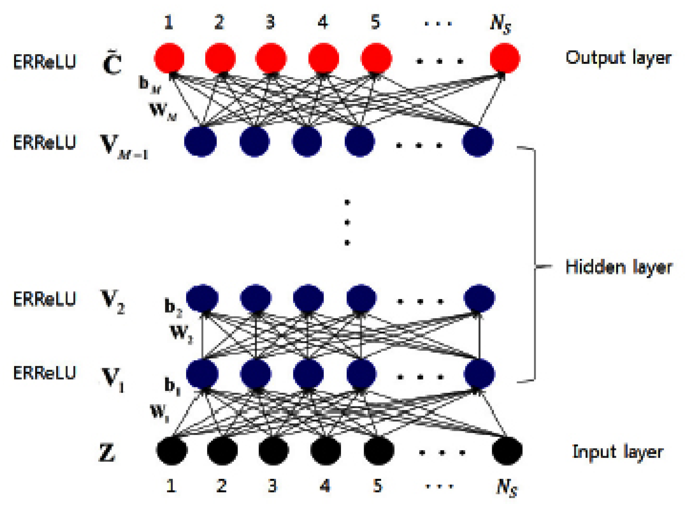
The entire network was smoothed through the aggregation of a convolution operation. Ultimately, as illustrated in
Figure 2, it was produced via the convolution layer as well as the polynomial kernel.
Every trainable characteristic is changed in the deleterious direction of the gradient with an adjustable step size given by a hyperparameter collectively called rate, and the gradients of the weight vector give the direction in which the function does have the sharpest rate of rise. The gradients are either of both the losses with regard to every learnable variable and a parametric iteration is written as follows in Equation (21) as well as Equation (22):
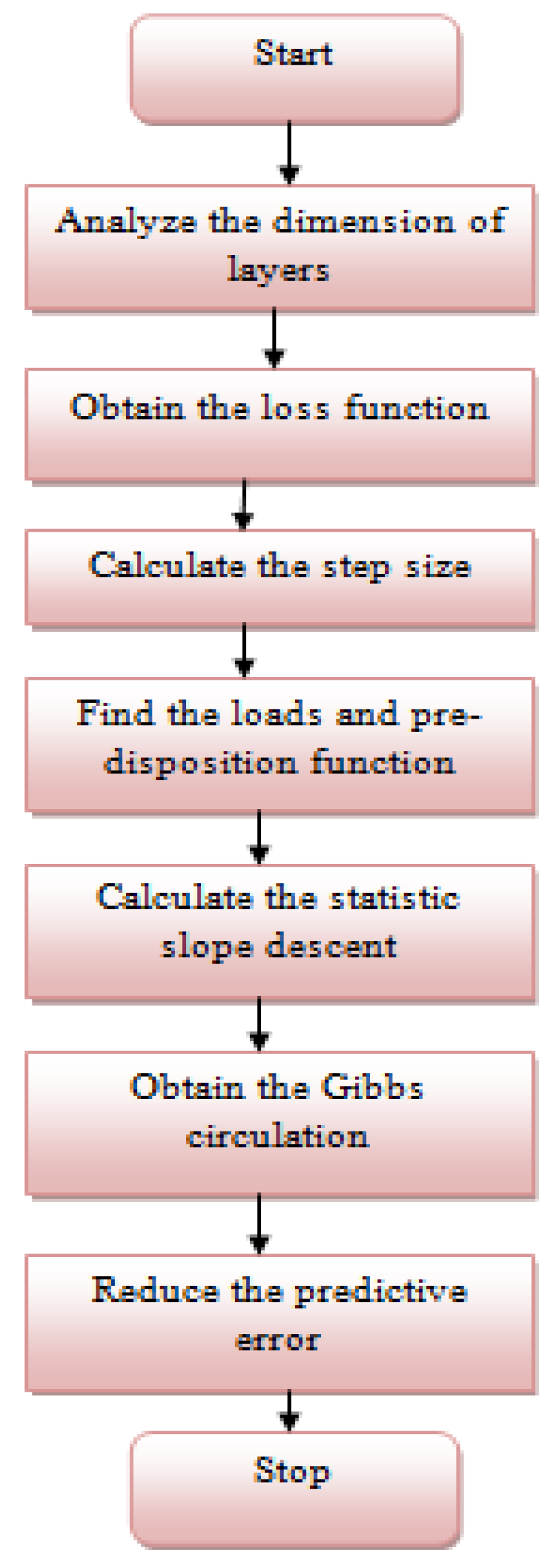
Figure 3 demonstrates the working flow of the proposed AUTO-NN for forecasting.
Where,
β is the parametric update rate,
x and
y are the weighted sum and offset vector for each tier, correspondingly, and (
a(
i),
b(
i)), 1 ≤
i ≤
N is a collection of samples Assuming the softmax has K neurons, with both the jth neurons assessing the prediction probability of class
j, provided the participation of
xH, which is the past layer’s output, and related to loads
W(
j) s as well as predilection
b(
j), as shown in Equation (23):
wherein,
xH is the previous layer’s payout. The created providing individualized expectations as shown in Equation (24) based on the probability assessment:
Over the large, statistical gradient decline greatly improved the variables 1, 2,...,
H,
s of the log-likelihood tragedy over the testing phase St. Parallel to ERReLU, our focus in this working framework, the irregularity factors (
V,
H) take esteem issues (
v,
h) ∈ {0, 1}
m+
n, and the combined probability distribution underneath the model. It is offered by the Gibbs circulatory with the vitality task presented in circumstance as shown in Equations (25) and (26)
Wij is a legitimate valued weight connected to the margin among components
Vjj and
Hii for all
ii 1,...,
n and
jj 1,...,
m, and
bjj and
cii are genuine esteemed inclination terms linked to the
jth. The predictor built from an ERReLU network has only correlations seen between the layer of hidden and noticeable components but among two factors from the same layer. As shown in Equations (27)–(29), the restricted probability of a single parameter becoming one could be calculated as the termination frequency of a (probability) neurons having parabolic initiating employment:
Gibbs sampling is particularly straightforward due to the independence of the components in a single layer: Rather than examining new qualities for all elements individually, the circumstances of all components in a thin layer can be simultaneously evaluated. As a result, Gibbs inspection can be done in just two phases: evaluating a state v for the obvious layer depending on p(v|h) as well as analyzing another state h for the input layers depending on p(h|v). Square Gibbs sample is another term for all of this.
4. Comparative Analysis
The proposed AUTO-encoder-based Neural Network (AUTO-NN) was evaluated among three standard models, namely Radial Belief Neural Network (RBNN), Deep Belief Network (DBN), and Artificial Neural Network (ANN), based on these parameters. For the purpose of analysis,
RMSE (Root Mean Square Error),
nRMSE (Normalized Root Mean Square Error),
MAE (Mean Absolute Error),
MaxAE (Maximum Absolute Error), and
MAPE (Mean Absolute Percentage Error) were selected as the parameters. Here MATLAB is the tool used to analyze the results and the proposed and existing models.
where
is the actual generated PV output and
is the predicted PV output.
is the total estimated points in the forecasting time period.
where
—capacity of each PV array for power generation.
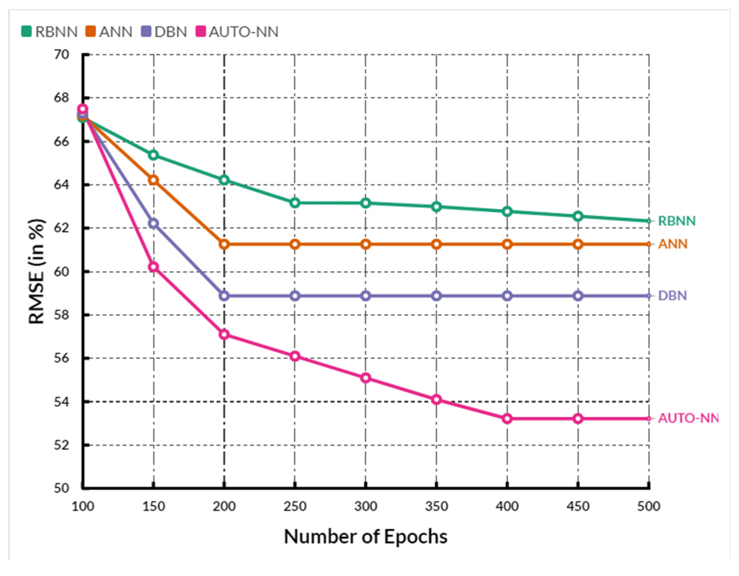
Figure 4 presents the comparison of
RMSE between the existing methods and the proposed method, in which the number of epochs used for analysis is given on the X-axis, and the
RMSE values in percentage are on the Y-axis. When compared, the existing RBNN, ANN, and DBN methods achieved
RMSE of 64%, 62.2%, and 60.52%, respectively. Comparatively, the proposed AUTO-NN method achieved an
RMSE of 58.72%, which is 6.72, 4.4, and 2.3 % lesser than the RBNN, ANN, and DBN methods.
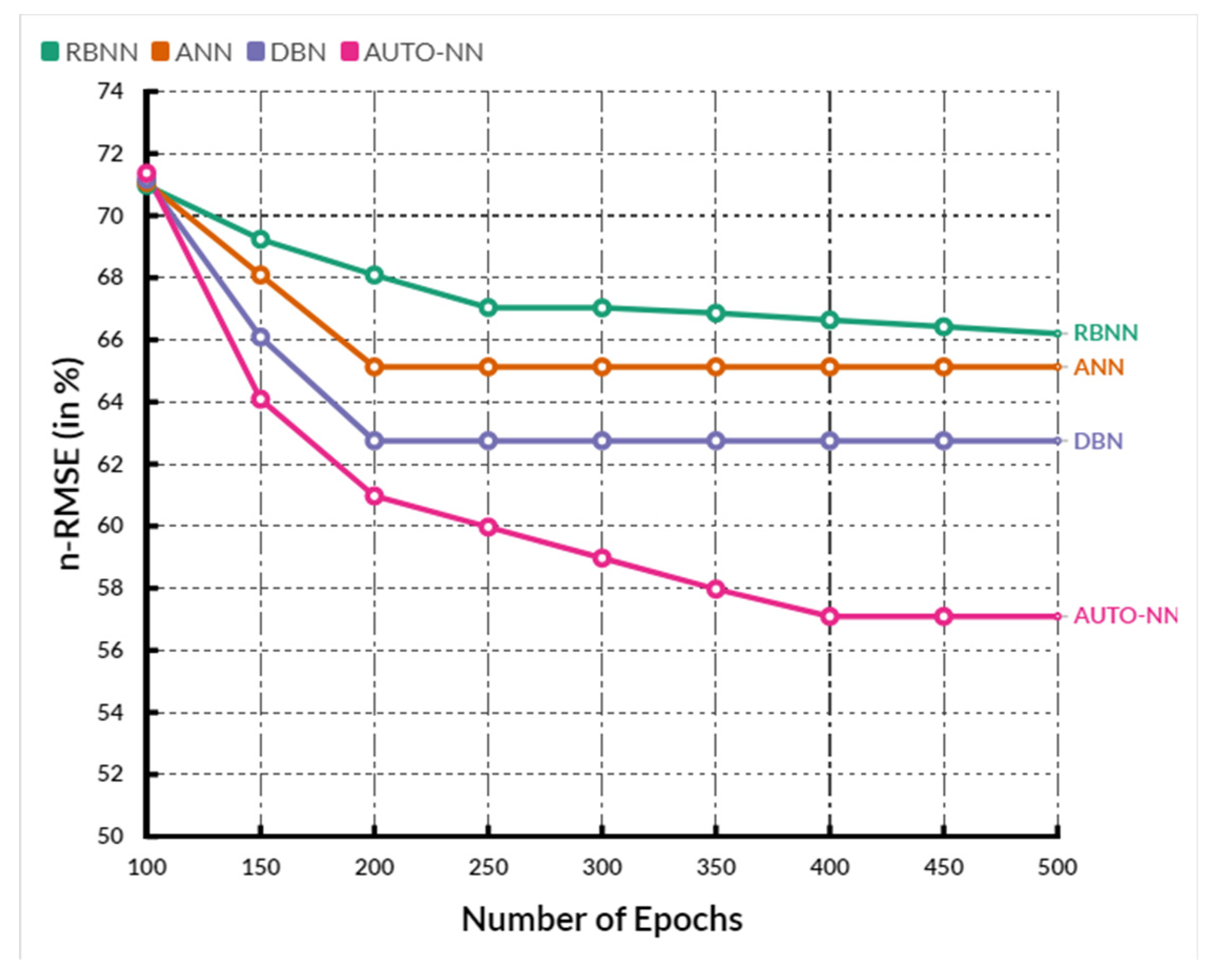
Figure 5 presents the comparison of
nRMSE between the existing RBNN, ANN, and DBN methods and the proposed AUTO-NN method. The X-axis displays the number of epochs used for analysis, and the Y-axis gives the
nRMSE values obtained in percentage. The existing RBNN, ANN, and DBNN methods achieved nRMSE of 67.48%, 66.58%, and 64.74%, respectively. In comparison, the proposed AUTO-NN method achieved an nRMSE of 62.7%, which is 5.36% lesser than RBNN, 4.5% lesser than ANN, and 2.02% lesser than the DBN method.
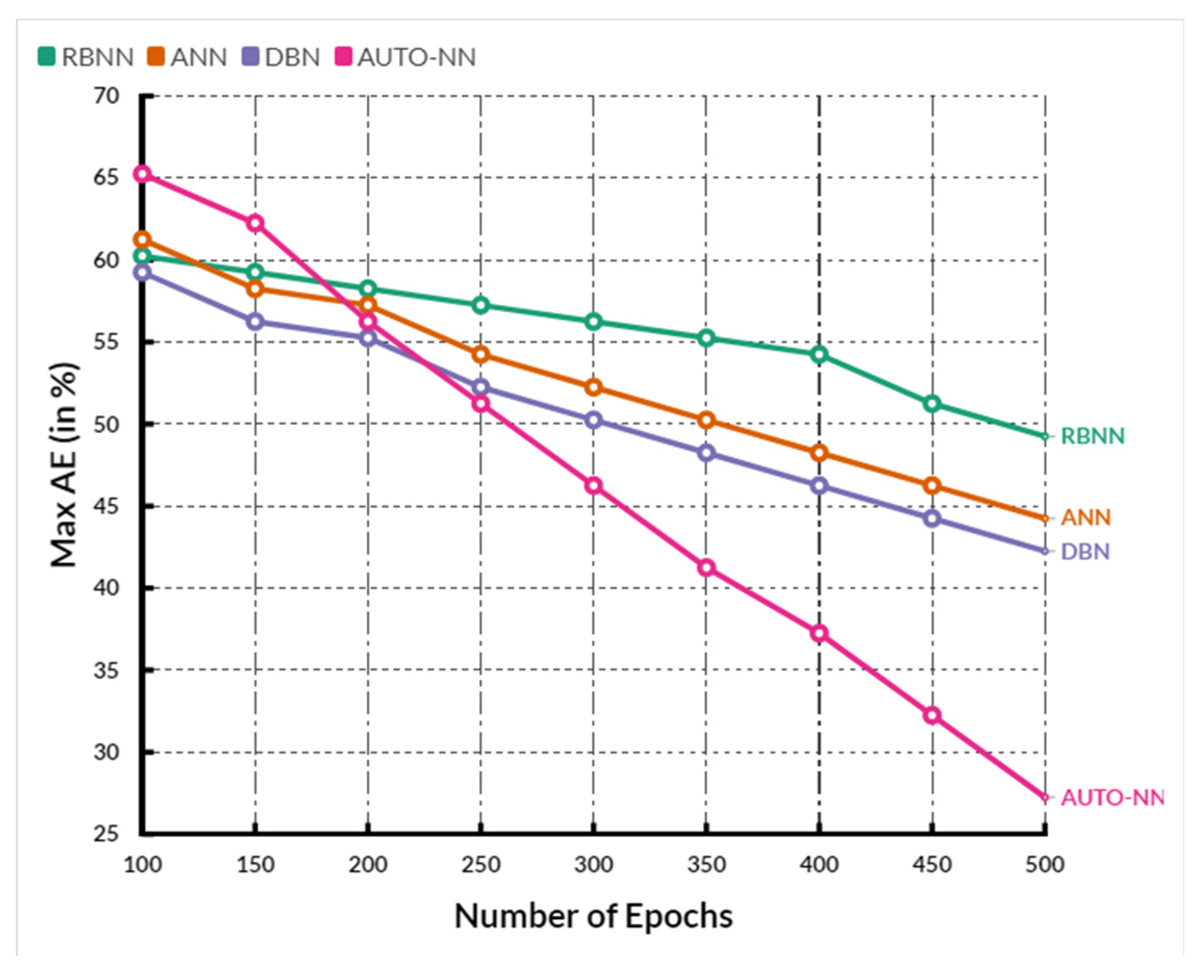
Figure 6 shows the comparison of
MaxAE between the existing RBNN, ANN, and DBN methods and the proposed AUTO-NN method, where the X-axis shows the number of epochs, and the Y-axis shows the
MaxAE values obtained in percentage. When compared, the existing RBNN, ANN, and DBN methods achieve 53.48%, 51.66%, and 50.54%, while the proposed AUTO-NN method achieves 48.04%, which is 5.44% better than RBNN, 3.62% better than ANN and 2.5% better than DBN.
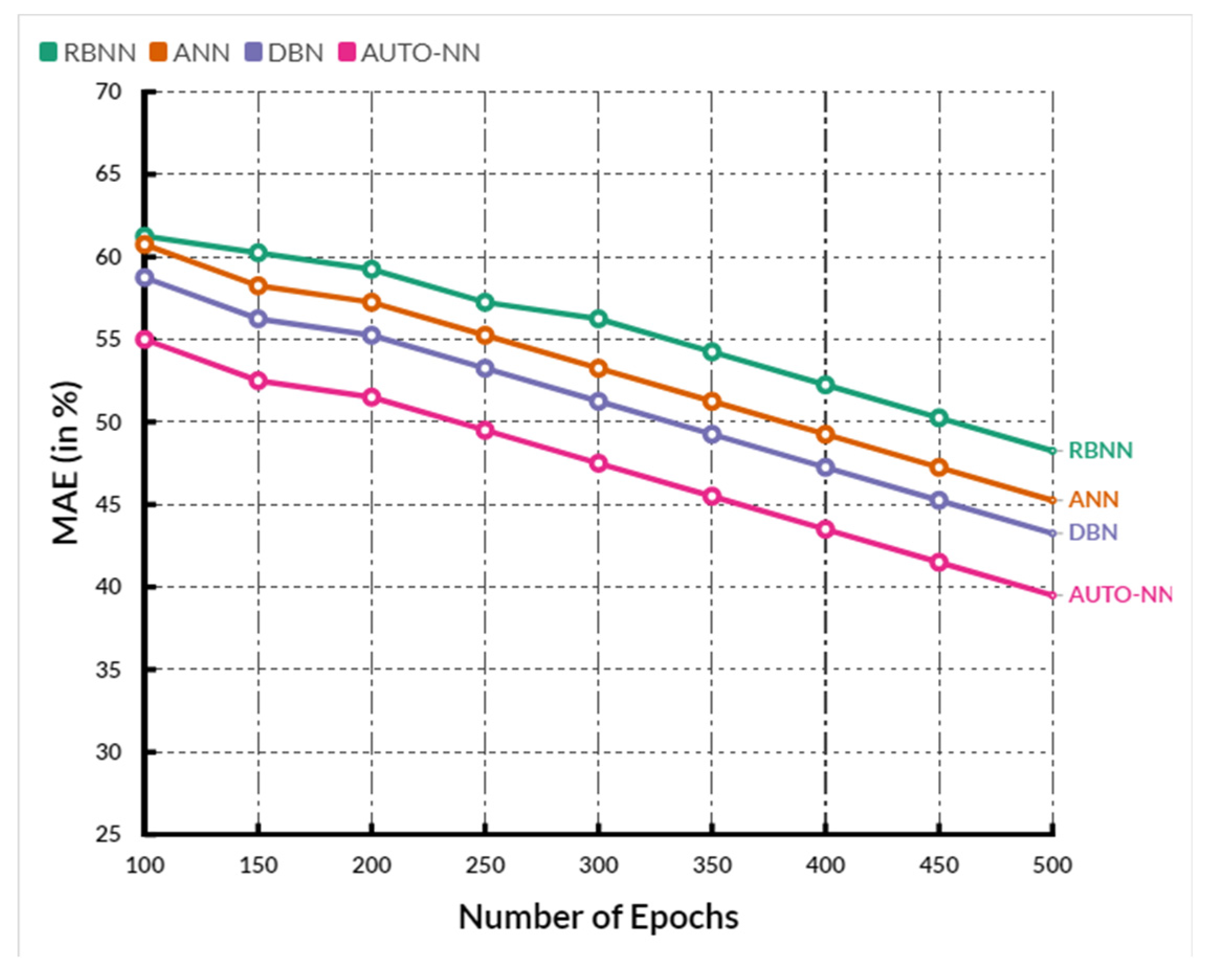
Figure 7 shows the comparison of
MAE between the existing RBNN, ANN, and DBN methods and the proposed AUTO-NN method, where the X-axis shows the number of epochs, and the Y-axis shows the MAE values obtained in percentage. When compared, the existing RBNN, ANN, and DBN methods achieve 57.26%, 56.2%, and 51.16%, while the proposed AUTO-NN method achieves 48.66%, which is 9.4% better than RBNN, 8.46% better than ANN and 3.5% better than DBN.
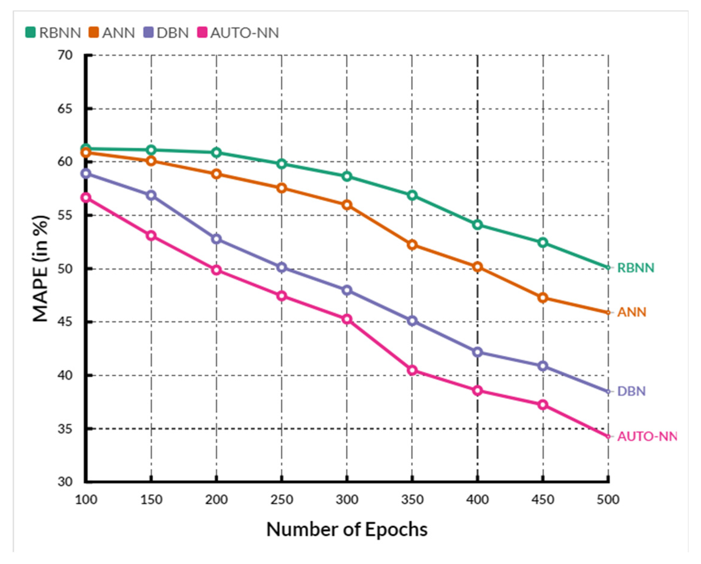
Figure 8 shows the comparison of
MAPE between the existing RBNN, ANN, and DBN methods and the proposed AUTO-NN method where the X-axis shows the number of epochs, and the Y-axis shows the
MAPE values obtained in percentage.
When compared, the existing RBNN, ANN, and DBN methods achieve 57.96%, 54.12%, and 48.96%, while the proposed method achieves 46.76%, which is 11.2% better than RBNN, 8.64% better than ANN and 2.2% better than DBN. The overall comparison between the existing and proposed model has shown in the following
Table 2In a comparison tip, the proposed AUTO-NN achieves 58.72% of RMSE (Root Mean Square Error), 62.72% of nRMSE (Normalized Root Mean Square Error), 48.04% of MaxAE (Maximum Absolute Error), 48.66% of MAE (Mean Absolute Error) and 46.76% of MAPE (Mean Absolute Percentage Error). While compared with the other existing models, the proposed model achieved better results.
The electricity produced by the solar panels is sent to the battery via an electronic controller, and the batteries store the energy. DC from the battery is inverted to AC; Electrical loads draw power from these batteries. In a straight-grid system (or grid-tied system), the SPV panels are connected to the public power supply lines through a controller and energy meter. No batteries are used here. Electricity is primarily used to power the household’s immediate power needs. When those requirements are met, a power meter sends additional power to the grid. Solar photovoltaic system cells convert only 10 to 14 percent of radiant energy into electrical energy. On the other hand, fossil fuel plants convert 30–40 percent of the chemical energy of their fuel into electrical energy. The conversion efficiency of electrochemical energy sources is as high as 90 to 95%.
Efficiency in a solar photovoltaic system is about 15%, meaning that for every 100 W/m
2 of radiation with 1 m
2 of the cell surface, only 15
W is transmitted to the circuit.
For lead-acid batteries, we can distinguish between two types of efficiency: coulombic efficiency and energy efficiency. During the charging process, which converts electrical energy into chemical energy, the Ah efficiency is about 90%, and the energy efficiency is about 75%
A large amount of solar and thermal energy makes it a beautiful energy source. This energy can be directly converted into direct current electricity and heat energy. Solar energy is the cleanest, most abundant, and inexhaustible renewable energy available on Earth. Solar panels or photovoltaic systems using panels (SPV panels) are placed on rooftops or solar farms arranged so that solar radiation falls on the solar photovoltaic panels to facilitate the reaction of converting sunlight into electricity. When pure silicon is at 0 K (0 degrees Kelvin–273 degrees Celsius), all positions in the outermost electron shells are occupied due to the absence of covalent bonds between atoms and the absence of free electrons. So the valence band is filled, and the conduction band is empty. Although valence electrons have the highest energy, they require the least energy to remove them from the atom (ionization energy). It can be illustrated with the example of a lead atom. Here the ionization energy (of a gas atom) of the first electron removal is 716 kJ/mol and that of the second electron is 1450 kJ/mol. The equivalent values for Si are 786 and 1577 kJ/mol.


