Article

High-Performance Computing and ABMS for High-Resolution COVID-19 Spreading Simulation

Department of Engineering and Architecture, University of Parma, 43124 Parma, Italy
*
Author to whom correspondence should be addressed.
Future Internet 2022, 14(3), 83; https://doi.org/10.3390/fi14030083
Submission received: 19 February 2022 / Revised: 7 March 2022 / Accepted: 9 March 2022 / Published: 11 March 2022
(This article belongs to the Special Issue Modern Trends in Multi-Agent Systems)

Abstract

:
This paper presents an approach for the modeling and the simulation of the spreading of COVID-19 based on agent-based modeling and simulation (ABMS). Our goal is not only to support large-scale simulations but also to increase the simulation resolution. Moreover, we do not assume an underlying network of contacts, and the person-to-person contacts responsible for the spreading are modeled as a function of the geographical distance among the individuals. In particular, we defined a commuting mechanism combining radiation-based and gravity-based models and we exploited the commuting properties at different resolution levels (municipalities and provinces). Finally, we exploited the high-performance computing (HPC) facilities to simulate millions of concurrent agents, each mapping the individual’s behavior. To do such simulations, we developed a spreading simulator and validated it through the simulation of the spreading in two of the most populated Italian regions: Lombardy and Emilia-Romagna. Our main achievement consists of the effective modeling of 10 million of concurrent agents, each one mapping an individual behavior with a high-resolution in terms of social contacts, mobility and contribution to the virus spreading. Moreover, we analyzed the forecasting ability of our framework to predict the number of infections being initialized with only a few days of real data. We validated our model with the statistical data coming from the serological analysis conducted in Lombardy, and our model makes a smaller error than other state of the art models with a final root mean squared error equal to 56,009 simulating the entire first pandemic wave in spring 2020. On the other hand, for the Emilia-Romagna region, we simulated the second pandemic wave during autumn 2020, and we reached a final RMSE equal to 10,730.11.

1. Introduction

In the earliest months of 2020, the unexpected COVID-19 spreading put all the world’s countries in difficulties because of the lack of countermeasures and knowledge about this novel virus to model its spreading. Moreover, since SARS-CoV-2 is an air-borne disease, it spreads among people due to everyday social interactions that represent themselves as a complex system to be modeled and simulated. Classical methods based on dynamic models like the Susceptible-Exposed-Infectious-Removed (SEIR) model [1,2] can only help with several limitations when high simulation resolution (fine-grained) is desired. Indeed, the class of SEIR models has to be extended to model particular conditions like social distancing, lockdown policies, and mask wearing. Although these extensions are easy to implement with additional equations in the basic model, these models do not still address the primary issue related to the basic reproduction number (R_0), which is not policy-invariant. Indeed, it depends on the average number of contacts among people, assuming that the population distribution is uniformly mixed. Moreover, the contact distribution is mixed heterogeneously in a natural population and shows some complex network characteristics.
Therefore, to avoid the problems of dynamic models, a different modeling and simulation approach should be used. Agent-based modeling and simulation (ABMS) is a better choice because it can model single individuals’ characteristics and behaviors with a common trade-off between resolution and population size [3]. This paper proposes a novel case study based on ABMS and on previous experiences to increase the simulation resolution in the same large-scale context of COVID-19 spreading in Italy. Therefore, to avoid the problems of dynamic models, a different modeling and simulation approach should be used. Agent-based modeling and simulation (ABMS) is a better choice because it can model single individuals’ characteristics and behaviors with a common trade-off between resolution and population size [3]. This paper proposes a novel case study based on ABMS and on previous experiences to increase the simulation resolution in the same large-scale context of COVID-19 spreading in Italy. The main contributions of our work are the following: (a) a software solution to model and execute millions of concurrent agents using the high-performance computing that maps individuals’ behavior to a high simulation resolution; (b) providing a simulator for COVID-19 based on our framework that reaches interesting performances when used to forecast new infections cases using only few days of real data for the initialization; and (c) we propose a commuting model that is suitable for the epidemic context but that can be reused also in different domains.
On the contrary to previous works, we did not assume an underlying network of contacts, modeling social meetings as a function of the geographical distance among the individuals exploiting the commuting properties at different resolution levels (municipalities and provinces). We defined a commuting mechanism combining two distance-based models: the radiation model [4] and the gravity model [5]. To achieve this goal, we implemented a spreading simulator using ActoDemic [6] and validated it on two of the most populated Italian regions: Lombardy and Emilia-Romagna. The next section shows the features of ABMS, and Section 3 introduces the main epidemic models. Section 4 discusses the use of actors in ABMS application. Section 4 introduces the case study and discusses the development. Section 5 and Section 6 discuss the features of our simulation model and introduces two simulation use cases. Section 7 discussed the results of the simulations of COVID-19 spreading in the Emilia Romagna and Lombardy regions. Finally, Section 8 concludes the paper by discussing its main features and the directions for future work.

2. Agent Based Modelling and Simulation

Agent-based modeling and simulation (ABMS) is a computational model for simulating phenomena in order to understand their behavior and what governs their results [3] and which exploits multi-agent systems and simulation models [7]. In particular, in an ABMS application, a simulation model is built on a generative and bottom-up process that integrates three types of components: the agents, who can perform one or more different behaviors, the environment in which the agents act by perceiving its state and acting accordingly, and, finally, the mechanisms that guide the interaction between the agents and exploit the direct and indirect exchange of information between system agents [8,9]. In particular, the generative and bottom-up nature of ABMS models offers great potential for addressing phenomena in which conventional modeling and simulation paradigms have difficulty in capturing their fundamental characteristics [10]. In fact, with an ABMS approach, instead of analyzing a phenomenon only in its entirety (as happens in discrete simulation systems), it is possible to analyze it, not only in its entirety but also in its components [11].
Furthermore, since a wide variety of research and application fields uses ABMS models, it follows that ABMS models can have very different characteristics when supporting the simulation of very different phenomena. According to [12], the most suggested ABMS models for complex systems modeling are cellular automata [13], flocking systems [14], and geographic information systems [15].
The success and diffusion of ABMS techniques is also due to the availability of software platforms that facilitate the development of models, the execution of simulations and the analysis of results [16,17,18,19]; in particular, among these software platforms, the best known and most used are: ASCAPE [20], MASON [21], Repast [22], AnyLogic [23] and NetLogo [24]. However, such platforms do not provide all the elements necessary to develop real intelligent agents, and so the development of the necessary models for some kinds of ABMS application may require the integration of an AI language (e.g., Prolog) or/and of some machine learning libraries. For example, Chumachenko et al. [25] proposed an intelligent information technology for integrating declarative languages and present an example of application that shows (i) how this technology allows the interoperability between NetLogo and Prolog, and (ii) how this kind of solution allows the resolution of decision-making problems and increases the efficiency of inference in a simulation environment.
Moreover, as introduced above, an important factor that can consolidate ABMS applications’ importance is the availability of software platforms that allow the development of highly complex and large-sized applications. A great deal of work has been done in this direction using compute clusters and graphics processing units (GPU)s. Among the main works, we can highlight [26,27,28,29,30]. However, the proposed solutions cannot solve all the problems that must be faced in developing complex ABMS applications with a large number of agents. This is due to many factors [31]; one of the most critical points is that the actions of agents drive the simulation, and each agent decided what to do by interacting with several other agents who, during the simulation, can always be the same or change, bit by bit, with a very high computational cost (n2) due to the need to identify the new agents at each simulation step. This is a big problem for applications running on a cluster of computers because, like this type of solution, execution is only effective if the processors spend most of their time processing rather than communicating [32]. Furthermore, it is often necessary to maintain the same order of execution of the agents to ensure the repeatability of the results, but in a multi-node system, this involves the use of synchronization protocols that at least increase execution times [33]. Finally, in such applications, the various agent’s creations may not be completely simple. In fact, it is possible to have sets of heterogeneous agents which probably require a different method of creation; it may be necessary to configure agents of the same type with different or random data, etc.

3. Agent Based Modeling and Simulation for Epidemic Scenarios

Different ABMS solutions have been proposed to model and solve real and complex epidemic scenarios and, in particular, COVID-19 spreading [34]. Dyke Parunak et al. [35] assert that such scenarios can be modeled both with agents (ABMS) and with equations (EBM), but also that: (i) ABMS is most appropriate for domains characterized by a high degree of localization and distribution and dominated by discrete decisions, and (ii) EBM is most naturally applied to systems that can be modeled centrally, and in which the dynamics are dominated by physical laws rather than information processing. Moreover, they foresee that ABMS will be offered better solutions than EBM if they will provide comparable tools for constructing and analyzing system dynamics models. Rahmandad and Sterman [36] demonstrated that stochastic ABMS can show better performance in respect to differential equation models, when several parameters are unknown and there is the need for capturing heterogeneity across individuals and their network of reciprocal interactions. Ajelli et al. [37] compare ABMS and meta-population strategies for modeling the epidemic in Italy, concluding that a trade-off between the two methods depends on data availability and suggesting the use of hybrid models.
Silva et al. [38] proposed an individual-based simulation model for exploring scenarios for COVID-19 where individuals are modeled as moving particles. In particular, COVID-19 infections take place when two particles come closer than a certain contact radius. Social distancing for COVID-19 is modeled as changes in the contact radius or introducing a momentum term. Hinch et al. [39] modeled COVID-19 spread by replacing the moving particles with contact networks for households, work, and random contacts. Their model should enable scientists and policymakers to quickly compare the effectiveness of non-pharmaceutical interventions like lockdowns, testing, quarantine, and digital and manual contact tracing. In particular, the model is experimented in an environment represented by a city with a default population of 1 million people whose ages and contact patterns are parameterized according to UK demographics. Moreover, the use of contact networks has been proposed by several researchers (see, for example, [40,41,42]). Truszkowska et al. [43] proposed a high-resolution model using single individuals’ features with real data about the COVID-19 outbreak in New Rochelle (NY), where thousands of citizens live. Moreover, they extend the typical simulation by modeling employees, hospitals, schools, and retirement homes and simulating the use of different test strategies, different types of treatment, and the presence of infections that cause similar COVID-19 symptoms. Finally, Chumachenko et al. [44] proposed an ABMS model that divides the individuals on the basis of their epidemic state (susceptible, exposed, infected and recovered); such conditions can be used to model the epidemic spread before the introduction of vaccination of the individuals. Individuals interact with each other and with the modeling environment, and transmission of morbidity and the transitions of individuals between states occur on the basis of probabilistic coefficients. These coefficients are determined experimentally on the basis of official statistics data on the incidence of COVID-19 coming from the Ukraine Health Center. The results of the simulations showed that the most effective measures to reduce epidemic dynamics are self-isolation of patients and tracking of contact individuals of the population, and that the isolation of the entire population is not necessary, but it is enough to isolate 80% of patients in the active phase.

4. Actor Based Modeling and Simulation

Actors are autonomous computational entities that can interact with other actors by exchanging asynchronous messages. When they receive any response, they can concurrently: send other messages, create new actors, and change their behavior to be ready to manage the next messages that they think to receive [45]. Moreover, actors have the suitable characteristics to define and implement the computational agents used in multi-agent systems and ABMS models [46]. Indeed, actors and computational agents share some characteristics: (i) both react to external stimuli (i.e., they are reactive), (ii) both act independently and exhibit control over their internal state (i.e., they are autonomous), and (iii) both interact through the exchange of asynchronous messages and through these messages they are able to coordinate and cooperate with each other (i.e., they are social) [47]. Therefore, the availability of some actor-based software frameworks can simplify the development of computational agents in domains where agents act dynamically, change their behavior, and need to coordinate or cooperate through direct interactions.

4.1. Using Actors for Large Scale ABMS Applications

Several researchers proposed interesting solutions for large scale ABMS applications. For example, Jang and Agha [48] proposed an actor-based software infrastructure, called the actor’s adaptive architecture. This infrastructure supports the construction of large-scale agent-based simulations and exploits some distributed computing techniques to optimize the distribution of the agents of the application on a network of computational nodes. Moreover, this software infrastructure uses some optimization techniques to reduce the amount of data exchanged between nodes and support dynamic agents’ distribution and search. Scheutz et al. [49] proposed a simulation environment, called SWAGES, that provides an automatic and dynamic distribution of simulations that supports the minimization of the simulation times. In particular, SWAGES allows the use of different programming languages for the definition of the agent models, and provides large data collections and data analysis techniques that can help to simplify the analysis of the results. Moreover, it provides a flexible scheduler offering automatic fault detection and error recovery mechanisms, and so improving the reliability of large-scale simulations. Cicirelli et al. [28] proposed the use of actors for the distribution of simulations on the Repast software platform [22]. In particular, they defined a software infrastructure that: (i) decomposes an application into subsystems (theaters), (ii) each subsystem hosts a set of actors and can be allocated on one of the computational nodes of the application, and (iii) supports agent migration, transparent location naming and efficient communication. Wittek and Rubio-Campillo [50] present an ABMS framework, called Pandora, that is designed for social scientists that uses HPC resources and implemented in the C++ programming language; moreover, Pandora provides a Python interface to the framework that should make possible the development of ABMS to people with minimal programming background. Pandora divides a simulation environment among different computer nodes, and each one of them will own a section of the environment and the agents located in this section. Moreover, data and agents located in the border between adjacent nodes will be copied and sent to neighbors at every time step of simulation, in order to keep data consistent in all the execution. Pandora was used for experimenting the tradeoff of replacing a traditional cluster with a cloud solution. Since the simulation framework requires a high-speed interconnection, this solution should provide low performance, but a cloud cluster should reduce losses and prove that even a cheap cloud cluster can provide interesting computational power for the simulations. However, the experimentation showed that the use of a cloud environment can provide a cost-effective solution. Collier and North [51] proposed an ABMS system, called Repast HPC, that extends the Repast framework (North and Collier, 2006), and is developed in C++ and uses Message Passing Interface (MPI) [52] for supporting large-scale distributed computing. In particular, Repast HPC is an environment where several processes are running in parallel and where a massive number of agents can be distributed across such processes. This is possible because each process has its own scheduler for processing the local events and all the schedulers are synchronized. Finally, Repast HPC allows the definition of a shared context for each process that can host local agents and remote agents copied from another process. This solution should improve simulation performance because the interaction among local and remote agents of the same shared context does not need remote communication. Fan et al. [53] presented an automated HPC system, named DRAS (Deep Reinforcement Agent for Scheduling), that takes advantage of deep reinforcement learning. In particular, DRAS implements a hierarchical neural network that provides some important HPC scheduling features such as resource reservation and backfilling. Each DRAS execution is driven by a specific scheduling objective, and during the execution the system automatically learns to improve its policy through interaction with the scheduling environment and dynamically adjusts its policy as workload changes. The results of its experimentation seem to outperform the existing heuristic and optimization solutions by up to 45%. Finally, Santana et al. [54] proposed a scalable simulator, called InterSCSimulator, to support the simulation of complex and large-scale smart city scenarios. Additionally, in this case, the simulation is based on actors, and each actor models a car or a bus moving in the city from an origin to a destination vertex in the city graph. The experimentation results show that the simulator is scalable and easy to use. Moreover, this simulator supports the analysis of the results of the simulation by generating charts and animated simulations.

4.2. ActoDeS

ActoDeS (Actor Development System) is a framework for the development of distributed systems [55]. This framework is based on the use of concurrent objects (from here named actors) whose main characteristics derive from the actor model [45]. In ActoDeS, an actor is created by another actor; after its creation, the actor can interact with other actors through the exchange of asynchronous messages and, as a consequence, can change its behavior several times; once its work is finished, the actor kills itself. Moreover, an actor keeps messages received and not yet processed in a queue. ActoDeS is implemented using the Java language and allows the development of applications that, depending on the complexity of the application and the availability of hardware, software, and communication resources, can be distributed on one or more computational nodes. Three other main elements are involved in an ActoDeS application: actor spaces, management services, and actor services. In particular, an actor space acts as a “container” for a set of actors and supports their execution through the use of management and actor services. Moreover, in an application involving several actor spaces, each actor space is deployed in a different Java virtual machine. Therefore, an application involving multiple actor spaces can be distributed over multiple computational nodes. Moreover, the actors of an application can interact through point-to-point, broadcast, multicast and publish-subscribe messaging.

4.3. Using ActoDeS for ABMS Large Scale Applications

As previously introduced, the need to use ABMS in different research and application sectors, makes the availability of ABMS that offer the features necessary in the specific research and application domain. To address this problem, ActoDeS provides several implementations of the actors and components that define an application’s runtime. In particular, an actor can have its thread of execution or share it with the other actors of the actor space; moreover, different types of actors can perform simulation steps of different lengths during the execution of an application. Furthermore, as far as the runtime components are concerned, it is necessary to use different scheduling algorithms to guarantee good efficiency to different types of ABMS [56]. In this regard, ActoDeS provides some schedulers which implement the most interesting and well-known scheduling algorithms. These characteristics make ActoDeS a suitable means to build ABMS applications that, depending on the characteristics of the application domain, can be easily realized by choosing the implementations of the actors and runtime components most suitable for that type of application.
ActoDeS supports the development of large-scale ABMS applications by using specialized schedulers for distributed applications and using techniques to simplify and reduce the cost of communication. Among the various types of schedulers provided, a scheduler can remove an idle actor from the execution list, store it in persistent storage, and put it back into the execution list when the actor is ready to restart its execution. This type of scheduler is useful in application domains that involve many actors who, during the simulation, can have long periods of inactivity. In fact, in these conditions, the cost of removing, storing and adding actors can be easily balanced by reducing the number of actors running. In many cases, that solution guarantees a lower use of the hardware and software resources used by the application. Undoubtedly the most critical component to develop and ensure the proper functioning of ABMS applications, and especially of large-scale applications, is communication management. Regarding distributed applications, ActoDeS allows an actor to communicate transparently with actors from other actor spaces (i.e., it needs only to get their remote references). Regarding communication, ActoDeS supports, in addition to point-to-point communication, one-to-many communication via broadcast, multicast, and publish-subscribe protocols, and reduces the cost of one-to-one communication through message aggregation techniques [57,58].
Commonly, in different ABMS applications, each actor must propagate information to all or to a large part of the actors of the application. Naturally, if such messages were disseminated through a point-to-point interaction, the cost of communication would become intolerable even with a limited number of actors. However, ActoDeS provides an actor implementation, called “shared actor”, which avoids this type of problem: all the actors of the application share a single mailbox that keeps all the messages sent in the previous and current simulation step and allows the reception of the messages of the previous simulation step. Therefore, this type of actor can receive: (i) the point-to-point messages that are addressed to itself, (ii) all the broadcast messages, and (iii) all the messages from a multicast group to which it has subscribed. Furthermore, separating the messages of two simulation steps avoids the burden of keeping a copy of the current environment when it is necessary to ensure that agents decide their actions with the same information about the environment in which they operate [56]. In some cases, when there is a strong interaction between the application actors, especially when a relevant part of the interaction occurs between the actors of different computation nodes, the cost of communication can cause incorrect behavior or even the failure of the application.
ActoDeS seeks to reduce the cost of communication by adopting a message aggregation technique. This technique is managed by the managers of the different actor spaces and is applied to the messages that are sent to remote actors. In particular, each manager performs the following operations: (i) at the beginning of a simulation step it creates an aggregation message for each remote actor space; (ii) during the execution of the simulation step, inserts the messages addressed to other actor spaces in the appropriate aggregation message; (iii) at the end of the simulation step: (a) sends the appropriate aggregation message to each remote manager, (b) receives an aggregation message from each remote manager and (c) extracts the messages from each aggregation message and sends them to the (local) actors recipients.
A very important feature that an ABMS application development environment should be is the availability of graphical tools to visualize the evolution of simulations, and tools to analyze the data obtained from the simulations. ActoDeS does not provide tools for the visualization of simulations and the analysis of their results, but provides a logging service that allows the saving on a file of the streaming of Java objects that contain the data that describe the relevant actions of an actor (e.g., its initialization, reception, sending and processing messages, creating actors, changing behavior and its arrest). However, the processing of these logging files is quite simple, and therefore, it was not very difficult to create tools that supported these two types of functionality [59,60].

5. The Simulator

Our simulator is built using ActoDemic [6], which is a framework that aims to facilitate the design and development of spreading phenomena in large-scale scenarios. The base unit is represented by actors that, depending on the target application, represent the entities of the system to model and simulate. The actors are implemented using the Java framework ActoDeS as a backbone to support the agents’ concurrent execution and distribution over several nodes. Each individual is modeled using a Base Spreader (BS) actor, which has a set of default attributes that can be enabled, configured, and modified to best suit the model. These attributes represent the demographic knowledge we used to model the population, but also the hidden internal state of each individual:
  • Unique identifier
  • Province or municipality of residence
  • Age
  • Number of daily contacts
  • Current infection state
  • If the individual is an essential worker
  • If the individual wears a protective mask during the simulation period.
The last two parameters are necessary to model and simulate different conditions verified in the early stage of the pandemic in Italy between February and May 2020.
In order to model the COVID-19 spread, we adopted the SEIR model, which provides susceptible, exposed, infected, and recovered compartments, and modified it by adding two extra compartments: positive and quarantine. These phases are typical in the COVID-19 infection cycle. At the beginning, all are in the susceptibility state. At this stage, every individual can be infected by another one who is contagious. An individual who gets infected moves from a susceptibility state to an incubation state and remains in this state for a certain amount of time before moving into the next compartment, where it will become infected. An infected subject can spread the virus and infect other individuals. When the infection phase ends, the individual becomes positive. Being positive means that the virus was identified with a COVID-19 test. Due to this result, the individual will be forced into a quarantine state, limiting his/her contacts. After a certain time, a positive could heal or die. There is no death probability, but deaths follow the real death curve of the simulated use case taken into account. In particular, the incubation phase lasts from 7 to 14 days, the infectious phase from 3 to 7 days, and the positive phase from 14 to 30 days [61]. Figure 1 shows a diagram that summarizes the described infection cycle. Moreover, the distinction between positive and negative is necessary to model the use-case in 2020 since real-data refers only to infections found with a delay using the COVID-19 tests several days after the first symptoms [62].
Contagion is based on a specific transmission probability for each individual. This probability represents the likelihood of being in a condition that supports the virus spread. We use a general COVID-19 transmission probability (CTV) estimated in [6], but this probability is scaled by each individual depending on two other stochastic parameters that are related to the use of protective masks and their efficacy. We used statistics and masks’ efficacy presented in [63]. We considered three categories of masks: cloth, surgical, and N95 masks. Efficiency of a mask is evaluated in terms of inward and outward protection. According to [63], a mask’s inward efficiency could vary from 20% to 80% for cloth, 70–90% for surgical, and above 95% for N95 masks. On the other hand, outward efficiency could range from 0 to 80% for cloth masks, while surgical and N95 masks are 50–90% and 70–100% outwardly protective, respectively. The effectiveness of a generic mask is assumed to be equal to the average effectiveness of the three previous types. Figure 2 describes the contagion modeling.

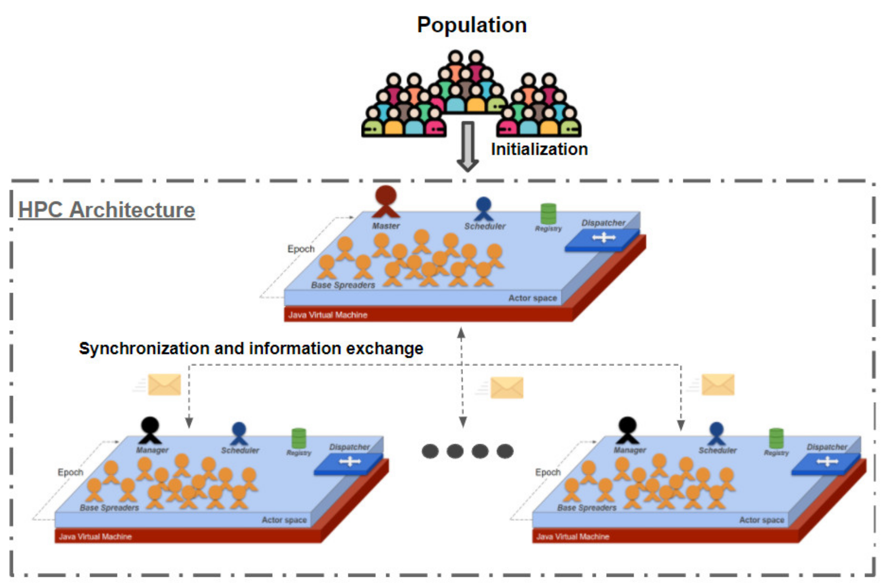
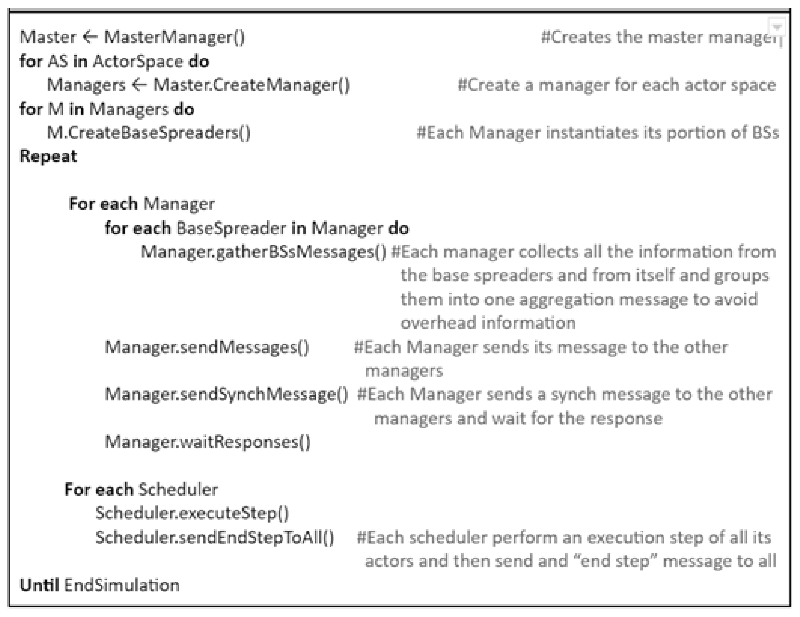
5.1. Software Architecture with HPC

Since each Base Spreader actor maps exactly one individual, we simulated 10 million agents for the Lombardy region and 5 million agents for the Emilia-Romagna region. Figure 3 shows the logical architecture of the simulator, that is described in the following lines. The simulation process is divided into several “epochs’’ representing a different day. Moreover, people can change their behavior depending on the current epoch (e.g., normal or lockdown). At the end of each epoch, the simulator provides a synchronization step to update the internal state (infectious state) of each BS depending on their meetings and according to an infectious probability we defined. The simulator involves a set of computational nodes whose execution is driven by a set of ActoDeS schedulers and managers. In particular, each manager has the duty of creating the subset of agents for its computational node and synchronizing the simulation execution on that node with the execution of the other computational nodes. Moreover, one of those managers assumes the role of “master” to partition the agents involved in the simulation, exchanging the information with the other managers to notify the agents under their control. We extensively used the ActoDeS passive actors for the BS implementation in order to allow large-scale development, while managers are active actors. The simulation process is described in Figure 4. The simulated population is divided into N actor spaces, where a manager assumes the duty of managing that portion in terms of execution and communication.
Finally, in each actor-space, there is an ActoDeS CycleScheduler that effectively manages the passive actors by coordinating their execution by exchanging messages with them until the end.
Every actor-space needs to exchange several pieces of information at the synchronization step. They exchange details about people’s meeting, people who must change their infection phase to “Incubated” due an infection, the number of people expected to die in their actor-space, other synchronization messages and finally an end signal. On the other hand, each manager sends to the Master only the currently positive individuals, infected individuals and a report related to the epoch processed. The high-performance computing system of the University of Parma offers various nodes with different characteristics. The one we used, involves two INTEL XEON E5-2683v4 2.1GHz processors (for a total of 32 cores) and 1024 Gb of RAM memory. The actors’ population is therefore divided into 32 actor spaces of 137,500 actors each. For Emilia Romagna (5 million agents), the average execution lasts 41 min and uses about 100 Gb of RAM memory. On the other hand, for Lombardy, the average execution lasts 3 h and 30 min and uses about 500 Gb of RAM memory.
We stochastically modeled COVID-19 spreading among two individuals by defining a specific transmission probability (TP) for this virus using the number of infections in the early autumn of 2020 when data were more accurate, rather than the beginning of the pandemic. This TP represents the ability of each BaseSpreader to transmit its state to another actor. Practically, the only actors that can transfer their state are the ones that are in the infectious or positive phases. Since we also modeled protective mask-wearing, the likelihood of infecting someone or being infected is a chain probability of TP, the Poutward (actor’s outward mask protection probability) and the Pinward (actor’s inward protection probability). Finally, the contagion happens by randomly sampling from a uniform distribution considering the contagion probability and actor’s susceptibility.

5.2. Commuting Model

To evaluate the robustness of our model and our hyper-parameters, we decided to add further detail to our model exploiting highly detailed data on socio-demographic structure in Italy and the commuting effects between provinces and municipalities. For high school students, university students and workers, there is the possibility that the employment place is located in a different town than that of residence, or even in a different province. Commuting is very common nowadays and plays an important role in the infection spreading even in the most isolated municipalities. Therefore, it is essential to model this phenomenon in a way that is as closely comparable to reality as possible. Commuting models commonly rely on the effectiveness of two parameters:
The grain: the finer the grain of the model, the more accurate the commuting model is.
The economic quotient: the most effective models take into account the economic quotient of every zone. Moreover, a municipality with a high number of businesses attracts more workers than another with few job opportunities.
After some analyses, we decided to use the average results between a gravitational model that is presented in [5] and the radial one that is explained in [4]. We chose this approach because the first model has a better commuters’ distribution in the various municipalities near the departure one. On the other hand, the second model computes in a more reliable way the correct number of people moving from a given municipality, but tends to distribute the contacts only to the closest town. The gravity model puts in a relationship the inhabitant number of the departure municipality, the inhabitant number of the arrival municipality, and the Euclidean distance between them:
c i , j = θ N i τ f N j τ t d i , j ρ
where:
  • c i , j is the probability that an individual living in i works or studies in municipality j
  • N i , N j number of individuals living in municipality i (or j)
  • θ proportional constant equal to 0.0005
  • τ f inhabitants damping constant of i equal to 0.28
  • τ t inhabitants damping constant of j which changes according to the number of people living in j:
    • 0.65 if the number of inhabitants is greater than 150,000
    • 0.66 if the number of inhabitants is between 5000 and 150,000
    • 0.78 if the number of inhabitants is less than 5000
  • d i , j distance between the municipalities i and j
  • ρ constant amplifying the dependence from distance which changes according to the number of people living in j:
    • 3.05 if the number of inhabitants is greater than 150,000
    • 2.95 if the number of inhabitants is between 5000 and 150,000
    • 2.5 0.78 if the number of inhabitants is less than 5000
Due to the lack of data of an economic quotient, we supposed that a municipality with many inhabitants also has a higher economic attraction. For this reason, the constants are set according to the number of people living in the municipality. The radial model, on the other hand, puts in a relationship the inhabitant number of the departure municipality, the inhabitant number of the arrival municipality, and the number of people living in the circle with a radius equal to the distance between the two municipalities. Hence:
p i , j = p i N i N j N i + S i , j N i + N j + S i , j
where:
  • p i , j is the probability that an individual living in i works or studies in municipality j
  • p i initial commuting probability of municipality i. This parameter can assume three different values according to the number of people who live in i:
    • if the number of inhabitants is greater than 150,000
    • 0.3 if the number of inhabitants is between 5000 and 150,000
    • 0.4 if the number of inhabitants is less than 5000
  • N i , N j number of individuals living in municipality i (or j)
  • S i , j population that lives within the circle with radius equal to the distance between i and j minus the population living in i and j
The values of the constants were identified by applying and comparing the model on the Italian scenario. Moreover, we identified the constants’ value using the data available from the Emilia Romagna region [61], and we combined this data with the features extracted from [5,6]. Figure 5 shows the difference between the gravity model and the radial one. In the first one, the Euclidean distance is enough to calculate the commuting probability between Albinea and Reggio nell’Emilia; in the second one, instead, we must also take into account the number of inhabitants contained in the area described by the circumference.

6. Use-Cases: Modeling the Emilia-Romagna and Lombardy Regions

To realize a working model for the Reggio Emilia province, we gathered data about contagion at the municipality level [61], and we also collected data about Emilia Romagna [62]. Unfortunately, we were not able to collect contagion data at the municipality level for the whole Emilia-Romagna region; therefore, to determinate our initial condition, we studied the Reggio Emilia province’s distribution, dividing the municipalities in different classes according to inhabitants’ number, then we extended this class format to the whole region. The geographical coordinates, mandatory for calculating the commuting model distance, was retrieved from [63], and the population size and distribution was provided by ISTAT [64].
To correctly tune the gravitation models and the radial ones, it is necessary to take into account the commuting values provided by the region [65]. The use case considered the second outbreak which affected the entire Italian territory. Therefore, the simulation period concerns the trend of infections between the 1 September 2020 and 15 December 2020. Finally, to validate our model, we compared with the official data provided by the Italian Government (Protezione Civile) and the regional government of Emilia-Romagna.

6.1. Social-Demographic Model

We introduced family groups and occupations (work or student) for the individuals involved in the simulation. In light of that, we can define a new socio-demographic model. The municipalities, with their geographical coordinates and the agents representing the population, are created following the data and probability distributions provided by the census. In our model, there are nine different family types, characterized by a different composition and number of members:
  • Single with children
  • Single without children
  • Single with children plus another adult
  • Couple without children
  • Couple without children plus another adult
  • Couple with children
  • Couple with children plus another adult
  • Adults that live together
  • Family groups (with at least one child)
With “other adult” we intended a person who is not strictly inside the family group but lives in the same habitation. Each type of family has a frequency of appearance, and the number of members may vary depending on a distribution probability shown in the Figure 6.
We introduced three fundamental constraints for building a consistent family group:
  • Any family group must contain at least one adult
  • The age of each child must be between 18 and 43 years less than the younger parent
  • The age difference of a couple is less than or equal to 15 years and they must be adult
We assigned an occupation to each individual based on its age. Moreover, we exploited some probability distributions based on the attendance rate. Finally, we implemented six different school categories, each with a specific attendance rate:
  • Kindergarten, attendance rate: 90%
  • Preschool, attendance rate: 90%
  • Elementary school, attendance rate: 100%
  • Middle school, attendance rate: 100%
  • High school, attendance rate: 92%
  • University, attendance rate: 31%
We have divided the students into classes, with different sizes depending on their category:
  • Kindergarten: 40 children
  • Preschool: 20 children
  • Elementary school: 19 children
  • Middle school: 21 lads
  • High school: 21 lads
  • University: 34 lads
On the other hand, as for workers, we considered different employment rates based on their age:
  • 15–19 years: 8%
  • 20–26 years: 30%
  • 27–34 years: 62.5%
  • 35–54 years: 73.5%
  • 55–70 years: 54.3%
We grouped workers into job groups, which can be of seven different types that differ according to the number of employees:
  • Very small company: up to 5 employees
  • Small company: up to 9 employees
  • Small-medium company: up to 19 employees
  • Medium company: up to 49 employees
  • Medium-large company: up to 99 employees
  • Large company: up to 249 employees
  • Very large company: over 250 employees
Each type of company has a different frequency of appearance, shown in Figure 7.

6.2. Restrictions

In Emilia Romagna’s model, there were six different levels of restrictions to represent as precisely as possible the division into bands implemented by the Italian government during the simulation period taken into account:
  • White: no restrictions
  • White from 10/18 to 10/24: represents the restrictions introduced on 18 October 2020: no limitations regarding work, but high schools and universities at 50% in attendance. The number of daily interactions is reduced by 40% to shape the closure of businesses such as bars after 9 pm and restaurants after midnight.
  • White from 10/25 to 11/05: represents the latest restrictions introduced before the zoning: no limitations regarding work, but schools and universities still at 50% in attendance. Closing of activities such as gyms, theaters and cinemas, closing restaurants after 6 pm, also the recommendation not to move. The number of social interactions is reduced by 50% compared to the initial value.
  • Yellow: high schools and universities closed (100% distance learning). Curfew from 22.00. Closure to the public of exhibitions, museums and other places of culture such as archives and libraries. To model these additional restrictions, the number of social interactions is reduced by 60%.
  • Orange: in addition to the limitations of the yellow area, the prohibitions on moving between municipalities except for proven work needs and the closure of catering activities (excluding take-away) are added. The use of smart working is encouraged and recommended even for workers, excluding essentials. In the model, social interactions are reduced by 70% compared to the initial values and cannot take place outside the municipalities (except those related to work activities).
  • Red: in addition to the limitations of the orange zone, the prohibition of movement within the municipality. For this, the daily interactions are reduced by 80% and reduced to zero those regarded as usual ones.

6.3. Spreading Parameters’ Selection

To correctly model the contagion evolution, we had to tune the simulator transmission probability, which is a fundamental ActoDemic parameter [6]. We determined it with an empirical procedure: we computed the average of ten simulations for every parameter’s value and we searched for the optimal value with a random search across the probability space, trying to chase up the real data curve in Reggio Emilia’s province (see Figure 8) and even in Emilia Romagna region (see Figure 9).
For Reggio Emilia’s province, the TP optimal value was 0.285. Moreover, the TP value identified for Reggio Emilia’s province was too high when applied to the whole Emilia Romagna scenario. The reason was identified to be due to the commuting mechanism. In fact, each province is also influenced by the contagions of the other provinces. Therefore, we searched for a new TP value which could be suitable for the region scenarios, and then we found 0.25 as the optimal value.

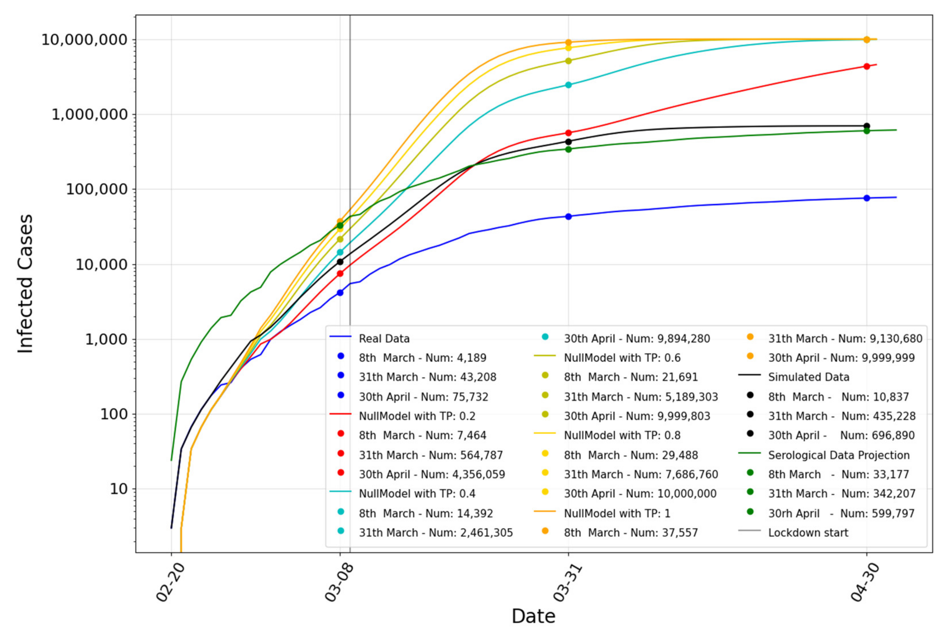
6.4. Results for Emilia-Romagna

After finding an optimal TP for the two considered use cases, we simulated the scenarios again. We highlighted when the restrictions, implemented in the simulator, are enabled. First, we simulated the Reggio Emilia province scenario with a TP equal to 0.285. We took into consideration the daily infections trend (see Figure 8), obtaining an R2 equal to 0.854, a Pearson correlation equal to 0.941, and an RMSE equal to 48.32 (see Figure 10).
The simulated curve has a very similar trend compared to the real one, which is however very disturbed mainly due to the dissimilarity in the number of daily COVID-19 tests performed in the province. For this reason, we had to create a cumulative curve to better limit data pollution. We got, in this case, an R2 equal to 0.986, a Pearson correlation equal to 0.9988, and an RMSE equal to 608.88 (see Figure 11).
Secondly, we simulated the use case considering the entire territory of Emilia Romagna. The TP taken into consideration in this case was 0.25. However, we also considered both daily and incremental infections trends. In Figure 12, it is possible to see the curve concerning the daily infections in the region. We obtained an R2 score of 0.881, a Pearson correlation of 0.977, and an RMSE of 319.08. Moreover, for the incremental representation of the infections in Figure 13, we obtained an R2 of 0.922, a Pearson correlation of 0.9993 and an RMSE 10,730.11.
We can infer that the simulator is performing and reliable, and thanks to the achieved result, we can say that our commuting model simulates at best the movement of agents within a bi-dimensional space, whether this space is a province with its municipalities or an entire whole region. Therefore, the simulator can be used to verify the effectiveness of the restriction and predict if they will be effective for lowering the epidemiological curve’s trend.

6.5. Results for the Lombardy Region

For the Lombardy region case study, there were no high-resolution data for municipality, rather it was only available at the province level. For this reason, we extended all the features already validated for Emilia-Romagna using the 10 provinces of Lombardy. Moreover, according to [6], we decided to simulate for this case study the first pandemic wave between the 20 February 2020 and the 30 April 2020. We implemented the commuting algorithm considering each province as a large and single urban center. As previously reported, during the first pandemic period, real data about new infections were affected by the small capacity of doing a large number of COVID-19 tests among people. Thus, real data were underestimated and were about eight times higher, as proven by the serological analysis led by Italian institutions in July 2020 [6]. In light of this, we considered the real data contagion incremental curve and a curve representing a serological data projection representing a rough estimate of the neglected and never traced positives from the COVID-19 tracking activity. In Figure 14, it is possible to see how the commuting curve (in black) is very close to our estimation (in green), even though there is no social structure anymore that supports the agents’ meeting activity. Moreover, for completeness, we also reported our previous results (in red); this data was obtained using a power-law social network structure. Qualitative data comparison is shown in Table 1. Finally, to validate our model, we compared the simulation data with the official data provided by the Italian Government (Protezione Civile), named “Real Data”. Considering that the official data have been recognized as seriously underestimated in the first wave of the pandemic due to the lack of molecular tests, we decided to compare with the results provided by the serological investigation led by the Italian authorities over the Lombardy population in July 2020 to understand the real impact of the spreading in the previous months (serological data).
From the data qualitative analysis, it is clear that even the simulation that points the foundations of its social network on commuting mechanisms are plausible and acceptable, proving the robustness of the implemented ABMS model.

7. Discussion

We carried out further tests and simulations in order to validate our model. The realized high-resolution model takes into consideration many factors and parameters to tune up the infection spreading process (see [6] for better understanding how we used it). In particular:
  • The contagion susceptibility by age
  • The protection achieved thanks to wearable protective devices
  • The quarantine mechanism
Moreover, we analyzed how these parameters affect the spreading procedure. Hence, we created a model that does not take these parameters into consideration, but makes the infection process dependent only on transmission probability, without any additional damper. Figure 15 shows different infection trends with different TP values. Considering also the values reported in Table 2, we can assert that the parameters in our model create a sufficient contagion dampening, validating our infection process modeling.
We continued our analysis with further studies. For validating our model, we compared our results with other SEIR models. The comparison is shown in Figure 16. We took into account three different SEIR models. The first one (SEIR 1 in Figure 16) is a simple based system dynamics SEIR [2]. The second one [66] (SEIR 2 in Figure 16) takes into account the transmission rate of asymptomatic subjects and a piecewise exponentially-decreasing R0. The third one [67] (SEIR 3 in Figure 16) optimizes the model’s parameters using computational swarm intelligence to model the early stage of the pandemic in Italy. Moreover, we presented in Table 3 a numerical analysis of these models compared with ours. The chart and the analysis showed that our model produces a more accurate prediction of the infection spreading in terms of RMSE and the Pearson correlation.

8. Conclusions

In this paper, we introduced an approach for modeling and simulating large-scale complex systems exploiting an ABMS approach and the high-performance computing with a high-resolution. In particular, we modeled as a use-case the spread of COVID-19 across two Italian regions (Lombardy and Emilia-Romagna). To prove the efficacy of our solutions, we implemented a fine-grained model that takes into account single individuals with a socio-demographic model that also involves a novel commuting model to model for this kind of simulation. The results prove that this kind of solution is be able to solve complex tasks like predicting COVID-19 by exploiting the light-weight actor model and HPC. The results we obtained for both cases Lombardy (RMSE 56,009 during spring 2020) and Emilia-Romagna (RMSE 10,730 simulating autumn 2020) with respect to the real data suggest that the epidemiological domain can really benefit from such kinds of simulations, especially at the beginning of a spreading phenomenon when few reliable data are available. In particular, our ABMS model offers some interesting features which distinguish it from other ABMS: (i) the scheduling of the agents is driven by the messages exchanged from the agents of the application. In particular, at each step of execution an agent can receive more messages, but it can only process the messages received in the previous step; therefore, the behavior of the agents never depends on the order of execution of the agents during a simulation step. (ii) The availability of “remote proxy” reference provided by ActoDeS simplifies the development of agent-based applications because developers do not have to worry if an agent needs to communicate with some local agents or even with some remote agents, (iii) The use of aggregation messages guarantees a strong reduction in the cost of communication and, therefore, allows the development of real large-scale applications. Finally, in our future works, we would like to also stress these large-scale modeling capabilities in other domains and with complex tasks like financial simulation [68], temporal graph-based tasks [69,70] and troll detection [71,72], and also to refine our simulation models [73] and extend ActoDeS, taking advantage of some features offered by the JADE framework [74].

Author Contributions

Conceptualization, A.P.; methodology, M.P. and G.L.; software, M.P.; validation, S.C.; writing—original draft preparation, A.P., M.P. and G.L.; writing—review and editing, S.C.; supervision, A.P. All authors have read and agreed to the published version of the manuscript.

Funding

This research has been partially supported by the Supercomputing Unified Platform Emilia-Romagna—SUPER project.

Data Availability Statement

Not applicable.

Conflicts of Interest

The authors declare no conflict of interest.

References

  1. Li, M.Y.; Muldowney, J.S. Global stability for the SEIR model in epidemiology. Math. Biosci. 1995, 125, 155–164. [Google Scholar] [CrossRef]
  2. He, S.; Peng, Y.; Sun, K. SEIR modeling of the COVID-19 and its dynamics. Nonlinear Dyn. 2020, 101, 1667–1680. [Google Scholar] [CrossRef] [PubMed]
  3. Macal, C.M.; North, M.J. Tutorial on agent-based modeling and simulation. In Proceedings of the Winter Simulation Conference, Orlando, FL, USA, 4 December 2005. [Google Scholar]
  4. Simini, F.; González, M.C.; Maritan, A.; Barabási, A.L. A universal model for mobility and migration patterns. Nature 2012, 484, 96–100. [Google Scholar] [CrossRef] [PubMed]
  5. Xia, Y.; Bjørnstad, O.N.; Grenfell, B.T. Measles metapopulation dynamics: A gravity model for epidemiological coupling and dynamics. Am. Nat. 2004, 164, 267–281. [Google Scholar] [CrossRef]
  6. Pellegrino, M.; Lombardo, G.; Mordonini, M.; Tomaiuolo, M.; Cagnoni, S.; Poggi, A. ActoDemic: A Distributed Framework for Fine-Grained Spreading Modeling and Simulation in Large Scale Scenarios. In Proceedings of the 22nd Workshop “From Objects to Agents” (WOA, 2021), Bologna, Italy, 1–3 September 2021. [Google Scholar]
  7. Niazi, M.; Hussain, A. Agent-based computing from multi-agent systems to agent-based models: A visual survey. Scientometrics 2011, 89, 479–499. [Google Scholar] [CrossRef] [Green Version]
  8. Bandini, S.; Manzoni, S.; Vizzari, G. Agent based modeling and simulation: An informatics perspective. J. Artif. Soc. Soc. Simul. 2009, 12, 4. [Google Scholar]
  9. Bandini, S.; Manzoni, S.; Vizzari, G. Agent-based modeling and simulation. In Complex Social and Behavioral Systems: Game Theory and Agent-Based Models; Sotomayor, M., Pérez-Castrillo, D., Castiglione, F., Eds.; Springer: Berlin/Heidelberg, Germany, 2020; pp. 667–682. [Google Scholar]
  10. Epstein, J.M. Generative Social Science: Studies in Agent-Based Computational Modeling. In Princeton Studies in Complexity; Princeton University Press: Princeton, NJ, USA, 2007. [Google Scholar]
  11. Klügl, F.; Bazzan, A.L. Agent-based modeling and simulation. AI Mag. 2012, 33, 29. [Google Scholar] [CrossRef]
  12. Grimm, V.; Railsback, S.F. Individual-based modeling and ecology. In Princeton Series in Theoretical and Computational Biology; Princeton University Press: Princeton, NJ, USA, 2013. [Google Scholar]
  13. Wolfram, S. Cellular automata as models of complexity. Nature 1984, 311, 419–424. [Google Scholar] [CrossRef]
  14. Reynolds, C.W. Flocks, Herds and Schools: A Distributed Behavioral Model. Available online: https://dl.acm.org/doi/pdf/10.1145/37401.37406?casa_token=xKKdS6A0HnkAAAAA:Y_z7E8qgBvJFzBVuAJMKujqyHiAfjAj9lQdlIPYYMUaZOhsV_6dmTtx8lV9TU8Uq718OjAp1Wvgslg (accessed on 18 February 2022).
  15. Gimblett, H.R. Integrating Geographic Information Systems and Agent-Based Modeling Techniques for Simulating Social and Ecological Processes; Oxford University Press: Oxford, UK, 2002. [Google Scholar]
  16. Allan, R.J. Survey of Agent Based Modelling and Simulation Tools; Science & Technology Facilities Council: New York, NY, USA, 2010; ISSN 1362-0207. [Google Scholar]
  17. Tobias, R.; Hofmann, C. Evaluation of free Java-libraries for social-scientific agent based simulation. J. Artif. Soc. Soc. Simul. 2004, 7. Available online: https://www.zora.uzh.ch/id/eprint/115438/1/Robert%20Tobias%20and%20Carole%20Hofmann-%20Evaluation%20of%20free%20Java-libraries%20for%20social-scientific%20agent%20based%20simulation.pdf (accessed on 18 February 2022).
  18. Nikolai, C.; Madey, G. Tools of the trade: A survey of various agent based modeling platforms. J. Artif. Soc. Soc. Simul. 2009, 12, 2. [Google Scholar]
  19. Abar, S.; Theodoropoulos, G.K.; Lemarinier, P.; O’Hare, G.M. Agent Based Modelling and Simulation tools: A review of the state-of-art software. Comput. Sci. Rev. 2017, 24, 13–33. [Google Scholar] [CrossRef]
  20. Parker, M. Ascape: An Agent-Based Modeling Framework in Java. Available online: https://www.osti.gov/servlets/purl/795682-rnZK04/native/#page=158 (accessed on 18 February 2022).
  21. Luke, S.; Cioffi-Revilla, C.; Panait, L.; Sullivan, K.; Balan, G. Mason: A multiagent simulation environment. Simulation 2005, 81, 517–527. [Google Scholar] [CrossRef] [Green Version]
  22. North, M.J.; Collier, N.T.; Vos, J.R. Experiences creating three implementations of the repast agent modeling toolkit. ACM Trans. Model. Comput. Simul. 2006, 16, 1–25. [Google Scholar] [CrossRef]
  23. Borshchev, A.; Brailsford, S.; Churilov, L.; Dangerfield, B. Multi-method modelling: AnyLogic. In Discrete-Event Simulation and System Dynamics for Management Decision Making; Wiley: Hoboken, NJ, USA, 2014. [Google Scholar]
  24. Wilensky, U.; Rand, W. An Introduction to Agent-Based Modeling: Modeling Natural, Social, and Engineered Complex Systems with NetLogo; MIT Press: Cambridge, MA, USA, 2015. [Google Scholar]
  25. Chumachenko, D.; Meniailov, I.; Bazilevych, K.; Chumachenko, T. On intelligent decision making in multiagent systems in conditions of uncertainty. In Proceedings of the 2019 XI International Scientific and Practical Conference on Electronics and Information Technologies (ELIT), Lviv, Ukraine, 16–18 September 2019. [Google Scholar]
  26. Lees, M.; Logan, B.; Oguara, T.; Theodoropoulos, G. Simulating Agent-Based Systems with HLA: The Case of SIM_AGENT-Part II (03E-SIW-076). In Proceedings of the 2003 European Simulation Interoperability Workshop, Stockholm, Sweden, 14–19 September 2003. [Google Scholar]
  27. Massaioli, F.; Castiglione, F.; Bernaschi, M. OpenMP parallelization of agent-based models. Parallel Comput. 2005, 31, 1066–1081. [Google Scholar] [CrossRef]
  28. Erra, U.; Frola, B.; Scarano, V.; Couzin, I. An efficient GPU implementation for large scale individual-based simulation of collective behavior. In Proceedings of the 2009 International Workshop on High Performance Computational Systems Biology, Trento, Italy, 14–16 October 2009. [Google Scholar]
  29. Cicirelli, F.; Furfaro, A.; Giordano, A.; Nigro, L. HLA_ACTOR_REPAST: An approach to distributing RePast models for high-performance simulations. Simul. Model. Pract. Theory 2011, 19, 283–300. [Google Scholar] [CrossRef]
  30. Cordasco, G.; De Chiara, R.; Mancuso, A.; Mazzeo, D.; Scarano, V.; Spagnuolo, C. Bringing together efficiency and effectiveness in distributed simulations: The experience with D-MASON. Simulation 2013, 89, 1236–1253. [Google Scholar] [CrossRef]
  31. Lysenko, M.; D’Souza, R.M. A framework for megascale agent based model simulations on graphics processing units. J. Artif. Soc. Soc. Simul. 2008, 11, 10. [Google Scholar]
  32. Scheutz, M.; Schermerhorn, P. Adaptive algorithms for the dynamic distribution and parallel execution of agent-based models. J. Parallel Distrib. Comput. 2006, 66, 1037–1051. [Google Scholar] [CrossRef]
  33. Som, T.K.; Sargent, R.G. Model structure and load balancing in optimistic parallel discrete event simulation. In Proceedings of the Fourteenth Workshop on Parallel and Distributed Simulation, Bologna, Italy, 28–31 May 2000. [Google Scholar]
  34. Lorig, F.; Johansson, E.; Davidsson, P. Agent-based social simulation of the COVID-19 pandemic: A systematic review. JASSS J. Artif. Soc. Soc. Simul. 2021, 24, 5. [Google Scholar] [CrossRef]
  35. Dyke Parunak, H.V.; Savit, R.; Riolo, R.L. Agent-based modeling vs. equation-based modeling: A case study and users’ guide. In International Workshop on Multi-Agent Systems and Agent-Based Simulation; Springer: Berlin/Heidelberg, Germany, 1998; pp. 10–25. [Google Scholar]
  36. Rahmandad, H.; Sterman, J. Heterogeneity and network structure in the dynamics of diffusion: Comparing agent-based and differential equation models. Manag. Sci. 2008, 54, 998–1014. [Google Scholar] [CrossRef] [Green Version]
  37. Ajelli, M.; Gonçalves, B.; Balcan, D.; Colizza, V.; Hu, H.; Ramasco, J. Comparing large-scale computational approaches to epidemic modeling: Agent-based versus structured metapopulation models. BMC Infect. Dis. 2010, 10, 190. [Google Scholar] [CrossRef] [Green Version]
  38. Silva, P.C.; Batista, P.V.; Lima, H.S.; Alves, M.A.; Guimarães, F.G.; Silva, R.C. COVID-ABS: An agent-based model of COVID-19 epidemic to simulate health and economic effects of social distancing interventions. Chaos Solitons Fractals 2020, 139, 110088. [Google Scholar] [CrossRef] [PubMed]
  39. Hinch, R.; Probert, W.J.; Nurtay, A.; Kendall, M.; Wymant, C.; Hall, M. OpenABM-COVID19—An agent-based model for non-pharmaceutical interventions against COVID-19 including contact tracing. PLoS Comput. Biol. 2021, 17, e1009146. [Google Scholar] [CrossRef] [PubMed]
  40. Gabler, J.; Raabe, T.; Röhrl, K. People Meet People: A Microlevel Approach to Predicting the Effect of Policies on the Spread of COVID-19. Available online: https://www.econstor.eu/bitstream/10419/232651/1/dp13899.pdf (accessed on 18 February 2022).
  41. Wolfram, C. An agent-based model of COVID-19. Complex Syst. 2020, 29, 87–105. [Google Scholar] [CrossRef]
  42. Shamil, M.; Farheen, F.; Ibtehaz, N.; Khan, I.M.; Rahman, M.S. An agent-based modeling of COVID-19: Validation, analysis, and recommendations. Cogn. Comput. 2021, 1–12. [Google Scholar] [CrossRef] [PubMed]
  43. Truszkowska, A.; Behring, B.; Hasanyan, J.; Zino, L.; Butail, S.; Caroppo, E.; Jiang, Z.-P.; Rizzo, A.; Porfiri, M. High-Resolution Agent-Based Modeling of COVID-19 Spreading in a Small Town. Adv. Theory Simul. 2021, 4, 2000277. [Google Scholar] [CrossRef]
  44. Chumachenko, D.; Meniailov, I.; Bazilevych, K.; Chumachenko, T.; Yakovlev, S. On intelligent agent-based simulation of COVID-19 epidemic process in Ukraine. Procedia Comput. Sci. 2022, 198, 706–711. [Google Scholar] [CrossRef]
  45. Agha, G.A. Actors: A Model of Concurrent Computation in Distributed Systems; MIT, Cambridge Artificial Intelligence Lab: Cambridge, MA, USA, 1985. [Google Scholar]
  46. Kafura, D.; Briot, J.P. Actors and agents. IEEE Concurr. 1998, 6, 24–28. [Google Scholar] [CrossRef]
  47. Wooldridge, M. An Introduction to Multiagent Systems; John Wiley & Sons: Hoboken, NJ, USA, 2009. [Google Scholar]
  48. Jang, M.W.; Agha, G. Agent framework services to reduce agent communication overhead in large-scale agent-based simulations. Simul. Model. Pract. Theory 2006, 14, 679–694. [Google Scholar] [CrossRef]
  49. Scheutz, M.; Schermerhorn, P.; Connaughton, R.; Dingler, A. Swages—An Extendable Distributed Experimentation System for Large-Scale Agent-Based Alife Simulations. Available online: citeseerx.ist.psu.edu/viewdoc/download?doi=10.1.1.86.4219&rep=rep1&type=pdf (accessed on 18 February 2022).
  50. Wittek, P.; Rubio-Campillo, X. Scalable agent-based modelling with cloud hpc resources for social simulations. In Proceedings of the 4th IEEE International Conference on Cloud Computing Technology and Science, Taipei, Taiwan, 3–6 December 2012. [Google Scholar]
  51. Collier, N.; North, M. Parallel agent-based simulation with repast for high performance computing. Simulation 2013, 89, 1215–1235. [Google Scholar] [CrossRef]
  52. Clarke, L.; Glendinning, I.; Hempel, R. The MPI message passing interface standard. In Programming Environments for Massively Parallel Distributed Systems; Birkhäuser: Basel, Switzerland, 1994. [Google Scholar]
  53. Fan, Y.; Lan, Z.; Childers, T.; Rich, P.; Allcock, W.; Papka, M.E. Deep reinforcement agent for scheduling in HPC. In Proceedings of the 2021 IEEE International Parallel and Distributed Processing Symposium (IPDPS), Portland, OR, USA, 17–21 May 2021. [Google Scholar]
  54. Santana, E.F.Z.; Lago, N.; Kon, F.; Milojicic, D.S. Interscsimulator: Large-scale traffic simulation in smart cities using erlang. In Proceedings of the International Workshop on Multi-Agent Systems and Agent-Based Simulation, São Paulo, Brazil, 8–12 May 2017. [Google Scholar]
  55. Bergenti, F.; Poggi, A.; Tomaiuolo, M. An actor based software framework for scalable applications. In Proceedings of the International Conference on Internet and Distributed Computing Systems, Calabria, Italy, 22–24 September 2014. [Google Scholar]
  56. Mathieu, P.; Secq, Y. Environment Updating and Agent Scheduling Policies in Agent-based Simulators. In Proceedings of the 4th International Conference on Agents and Artificial Intelligence (ICAART), Algarve, Portugal, 6–8 February 2012. [Google Scholar]
  57. Brisolara, L.; Han, S.I.; Guerin, X.; Carro, L.; Reis, R.; Chae, S.I.; Jerraya, A. Reducing fine-grain communication overhead in multithread code generation for heterogeneous MPSoC. In Proceedings of the 10th International Workshop on Software & Compilers for Embedded Systems Nice France, New York, NY, USA, 20 April 2007. [Google Scholar]
  58. Wesolowski, L.; Venkataraman, R.; Gupta, A.; Yeom, J.S.; Bisset, K.; Sun, Y.; Kale, L.V. Tram: Optimizing fine-grained communication with topological routing and aggregation of messages. In Proceedings of the 43rd International Conference on Parallel Processing, Minneapolis, MN, USA, 9–12 September 2014. [Google Scholar]
  59. Poggi, A. Agent Based Modeling and Simulation with ActoMoS. In Proceedings of the 16th Workshop “From Objects to Agents” (WOA, 2015), Napoli, Italy, 17–19 June 2015. [Google Scholar]
  60. Lombardo, G.; Fornacciari, P.; Mordonini, M.; Tomaiuolo, M.; Poggi, A. A multi-agent architecture for data analysis. Future Internet 2019, 11, 49. [Google Scholar] [CrossRef] [Green Version]
  61. Riccio, A. Analysis of the SARS-CoV-2 epidemic in Lombardy (Italy) inits early phase. Are we going in the right direction? medRxiv 2020. [Google Scholar]
  62. Godio, A.; Pace, F.; Vergnano, A. Seir modeling of the italian epidemic of SARS-CoV-2 using computational swarm intelligence. Int. J. Environ. Res. Public Health 2020, 17, 3535. [Google Scholar] [CrossRef] [PubMed]
  63. COVID-19 Aggiornamento Quotidiano dei Dati-Provincia Reggio Nell’Emilia. Available online: https://www.ausl.re.it/covid-19-aggiornamento-quotidiano-dei-dati (accessed on 17 February 2022).
  64. Archivio GitHub COVID-19 Dati Regioni. Available online: https://github.com/pcm-dpc/COVID-19/tree/master/dati-regioni (accessed on 17 February 2022).
  65. Coordinate Geografiche Comuni Italiani. Available online: https://www.dossier.net/utilities/coordinate-geografiche (accessed on 17 February 2022).
  66. Istat. Available online: https://www.istat.it (accessed on 17 February 2022).
  67. Analisi Pendolarismo Comune per Comune della Regione Emilia Romagna. Available online: https://statistica.regione.emilia-romagna.it/servizi-online/rappresentazioni-cartografiche/pendolarismo/analisi-comune (accessed on 17 February 2022).
  68. Adosoglou, G.; Lombardo, G.; Pardalos, P.M. Neural network embeddings on corporate annual filings for portfolio selection. Expert Syst. Appl. 2021, 164, 114053. [Google Scholar] [CrossRef]
  69. Lombardo, G.; Poggi, A.; Tomaiuolo, M. Continual representation learning for node classification in power-law graphs. Future Gener. Comput. Syst. 2022, 128, 420–428. [Google Scholar] [CrossRef]
  70. Lombardo, G.; Poggi, A. A Scalable and Distributed Actor-Based Version of the Node2Vec Algorithm. In Proceedings of the 20th Workshop “from Objects to Agents” (WOA, 2019), Parma, Italy, 26–28 June 2019. [Google Scholar]
  71. Fornacciari, P.; Mordonini, M.; Poggi, A.; Sani, L.; Tomaiuolo, M. A holistic system for troll detection on Twitter. Comput. Hum. Behav. 2018, 89, 258–268. [Google Scholar] [CrossRef]
  72. Tomaiuolo, M.; Lombardo, G.; Mordonini, M.; Cagnoni, S.; Poggi, A. A survey on troll detection. Future Internet 2020, 12, 31. [Google Scholar] [CrossRef] [Green Version]
  73. Angiani, G.; Fornacciari, P.; Lombardo, G.; Poggi, A.; Tomaiuolo, M. Actors based agent modelling and simulation. In International Conference on Practical Applications of Agents and Multi-Agent Systems; Springer: Cham, Switzerland, 2018; pp. 443–455. [Google Scholar]
  74. Bergenti, F.; Caire, G.; Monica, S.; Poggi, A. The first twenty years of agent-based software development with JADE. Auton. Agents Multi-Agent Syst. 2020, 34, 36. [Google Scholar] [CrossRef]
Figure 1. Detailed scheme of our infection cycle.
Futureinternet 14 00083 g001
Figure 2. Stochastic contagion modeling.
Futureinternet 14 00083 g002
Figure 3. The simulator’s architecture on the High Performance Computing (HPC) architecture divides individuals in several actor spaces on different computational nodes.
Futureinternet 14 00083 g003
Figure 4. The simulation process algorithm.
Futureinternet 14 00083 g004
Figure 5. Image representing the difference between the gravity model and the radial one. In this example, we consider the municipality of Albinea (departure) and the municipality of Reggio nell’Emilia (arrival).
Futureinternet 14 00083 g005
Figure 6. Family type distribution chart with relative number of members.
Futureinternet 14 00083 g006
Figure 7. Distribution of work classes.
Futureinternet 14 00083 g007
Figure 8. Graph of daily infected persons with different TP values—Reggio Emilia province.
Futureinternet 14 00083 g008
Figure 9. Graph of daily infected persons with different TP values—Emilia Romagna region.
Futureinternet 14 00083 g009
Figure 10. Positives’ daily representation—Reggio Emilia province, Emilia Romagna region.
Futureinternet 14 00083 g010
Figure 11. Positives’ incremental representation—Reggio Emilia province, Emilia Romagna region.
Futureinternet 14 00083 g011
Figure 12. Positives’ daily representation—Emilia Romagna region.
Futureinternet 14 00083 g012
Figure 13. Positives’ incremental representation—Emilia Romagna region.
Futureinternet 14 00083 g013
Figure 14. Positives’ daily representation—Lombardy region.
Futureinternet 14 00083 g014
Figure 15. Simulation results without damping parameters with different transmission probability (0.2, 0.4, 0.6, 0.8, 1) (incremental representation—y-axis scale is logarithmic).
Futureinternet 14 00083 g015
Figure 16. Comparison among our model, the serological data, the real data and the SEIR models (incremental representation—y-axis scale is logarithmic).
Futureinternet 14 00083 g016
Table 1. Pearson correlation and root mean squared error (RMSE) of our model with respect to the serological data projection.
RMSEPearson Correlation
Simulated Data—Real Data398,0420.9903
Table 2. Comparison of our model to the null models in terms of root mean squared error (RMSE) and Pearson correlation n.
RMSEPearson Correlation
Simulated Data—Serological105,3430.9903
Null model with TP = 0.2–Serological1,301,6490.8674
Null model with TP = 0.4–Serological4,662,7230.9456
Null model with TP = 0.6–Serological5,840,1970.9805
Null model with TP = 0.8–Serological6,422,8190.9763
Null model with TP = 1–Serological6,759,5540.9616
Table 3. Comparison of our model to the SEIR models in terms of root mean squared error (RMSE) and the Pearson correlation.
RMSEPearson Correlation
Simulated Data—Serological105,3430.990
SEIR 1—Serological269,1970.769
SEIR 2—Serological270,0600.859
SEIR 3—Serological318,0340.713
Publisher’s Note: MDPI stays neutral with regard to jurisdictional claims in published maps and institutional affiliations.

