Article

Do Cryptocurrency Prices Camouflage Latent Economic Effects? A Bayesian Hidden Markov Approach †

by
Constandina Koki
1,*,
Stefanos Leonardos
2 and
Georgios Piliouras
2
1
Department of Statistics, School of Information Sciences and Technology, Athens University of Economics and Business, 10434 Athens, Greece
2
Engineering Systems and Design, Singapore University of Technology and Design, Singapore 487372, Singapore
*
Author to whom correspondence should be addressed.
A preliminary version of this paper appeared Decentralized 2019 and awarded with the Best Paper Award.
Future Internet 2020, 12(3), 59; https://doi.org/10.3390/fi12030059
Submission received: 17 February 2020 / Revised: 18 March 2020 / Accepted: 19 March 2020 / Published: 21 March 2020

Abstract

:
We study the Bitcoin and Ether price series under a financial perspective. Specifically, we use two econometric models to perform a two-layer analysis to study the correlation and prediction of Bitcoin and Ether price series with traditional assets. In the first part of this study, we model the probability of positive returns via a Bayesian logistic model. Even though the fitting performance of the logistic model is poor, we find that traditional assets can explain some of the variability of the price returns. Along with the fact that standard models fail to capture the statistic and econometric attributes—such as extreme variability and heteroskedasticity—of cryptocurrencies, this motivates us to apply a novel Non-Homogeneous Hidden Markov model to these series. In particular, we model Bitcoin and Ether prices via the non-homogeneous Pólya-Gamma Hidden Markov (NHPG) model, since it has been shown that it outperforms its counterparts in conventional financial data. The transition probabilities of the underlying hidden process are modeled via a logistic link whereas the observed series follow a mixture of normal regressions conditionally on the hidden process. Our results show that the NHPG algorithm has good in-sample performance and captures the heteroskedasticity of both series. It identifies frequent changes between the two states of the underlying Markov process. In what constitutes the most important implication of our study, we show that there exist linear correlations between the covariates and the ETH and BTC series. However, only the ETH series are affected non-linearly by a subset of the accounted covariates. Finally, we conclude that the large number of significant predictors along with the weak degree of predictability performance of the algorithm back up earlier findings that cryptocurrencies are unlike any other financial assets and predicting the cryptocurrency price series is still a challenging task. These findings can be useful to investors, policy makers, traders for portfolio allocation, risk management and trading strategies.

1. Introduction

What are cryptocurrencies? How do they compare to traditional financial instruments? Are they like traditional money, like commodities, a hybrid of the former or an utterly new type of asset that merit their own definition and understanding? Early research, mainly focusing on Bitcoin (henceforth BTC), provides mixed insights. While the creation of new BTCs resembles the mining process of gold—or precious metals in general—its attributes clearly differentiate it from conventional commodities [1]. The claim that BTC is fundamentally different from valuable metals like gold is also backed by Klein et al. [2] due to its shortage in stable hedging capabilities. Along with [3], Cheah and Fry [1] also argue that standard economic theories cannot explain BTC price formation and using data up to 2015, they provide evidence that BTC lacks the qualities necessary to be qualified as money. However, using GARCH models, Dyhrberg [4] demonstrates that BTC has similarities to both gold and the US dollar (USD) and somewhat surprisingly that it may be ideal for risk-averse investors. Also, while the BTC is useful to diversify financial portfolios—due to the negative correlation to the US implied volatility index (VIX)—it otherwise has limited safe-haven properties [5,6,7]. Using data from a longer period (between 2010 and 2017), Demir et al. [8] conclude the opposite, namely that BTC may indeed serve as a hedging tool, due to its relationship to the Economic Policy Uncertainty Index (EUI).
The fact that cryptocurrencies are different from any other asset in the financial market is further supported by [9,10,11]. High volatility, speculative forces and large dependence on social sentiment at least during its earlier stages—as measured by social media and Internet data (Google trends, Wikipedia searches and Twitter posts)—are qualified by many as some of the main determinants of BTC prices [12,13]. Yet, a large amount of price variability remains unaccounted for. Moreover, the proliferation of cryptocurrencies other than BTC that are supported by different technologies, i.e., variations of the standard Proof-of-Work distributed consensus of the BTC blockchain, e.g., [14], calls for a more comprehensive research approach. Despite the high documented correlation in the price of the various cryptocurrencies, it is highly debated whether this trend will also continue into future or not [15,16].
In the present paper, we make an effort towards understanding the correlation between a set of traditional assets and cryptocurrencies. We adopt an economic/financial perspective and use a set of 14 financial and economic predictors comprising main exchange rates (4 variables), equity indices (4 variables), commodity future prices (oil and gold) and economic uncertainty indicators (2 variables) along with 2 quasi-economic and 2 cryptocurrency specific variables: the hash rate which captures the amount of investment on mining equipment and hence accounts for the economic size of the network and the average block size which implicitly measures the amount of transactions and hence the activity in the respective cryptocurrency. All the variables and the applied transformations are summarized in Table 1. Also, we report the correlations between the explanatory variables in Table 2.
Earlier studies highlight the scarcity of results on cryptocurrencies other than BTC and underline the need for a better understanding of the entire cryptocurrency ecosystem and its properties (statistical and economic), see e.g., [11,17]. Studies that go beyond the BTC prices and confirm via various financial models the importance of using diverse cryptocurrencies—rather than a single one—in portfolio optimization include but are not limited to [18] and [15]. In view of the above, in the present study, apart from Bitcoin (BTC), we also focus on Ether (ETH), the native coin of the Ethereum blockchain [14,19], and currently the second largest cryptocurrency in terms of market capitalization [20]. Unlike the BTC blockchain, the Ethereum blockchain has been launched eponymously and is governed, or more aptly researched and developed, by the Ethereum Foundation [21], a non-profit organization-based in Switzerland. The architecture of the Ethereum ecosystem has far-reaching implications on its long-term development and sustainability that clearly differentiate it from BTC. Supporting smart contract execution—execution of code snippets that go beyond the simple monetary transactions of BTC—Ethereum has scheduled a transition from the currently computationally heavy Proof of Work (introduced by BTC and followed by most cryptocurrencies) to the computationally efficient alternative of Proof of Stake, which saves on energy resources and provides a scalable infrastructure while retaining the same security guarantees as Proof of Work. Without going further into the technical details, the main motivation to study ETH that stems from these considerations is the following. Given the different technological advancements that are promised by Ethereum, will ETH become independent from BTC and follow its own path as a cryptocurrency or are after all the values of all cryptocurrencies inevitably tied, as they are up to now [16]? Keeping in mind that ETH—i.e., the native coin—is only one of the main applications of the ETH blockchain—and the blockchain technology in general—it should also be noted that price movements of ETH may not necessarily align in the future with technological advancements in the Ethereum blockchain.
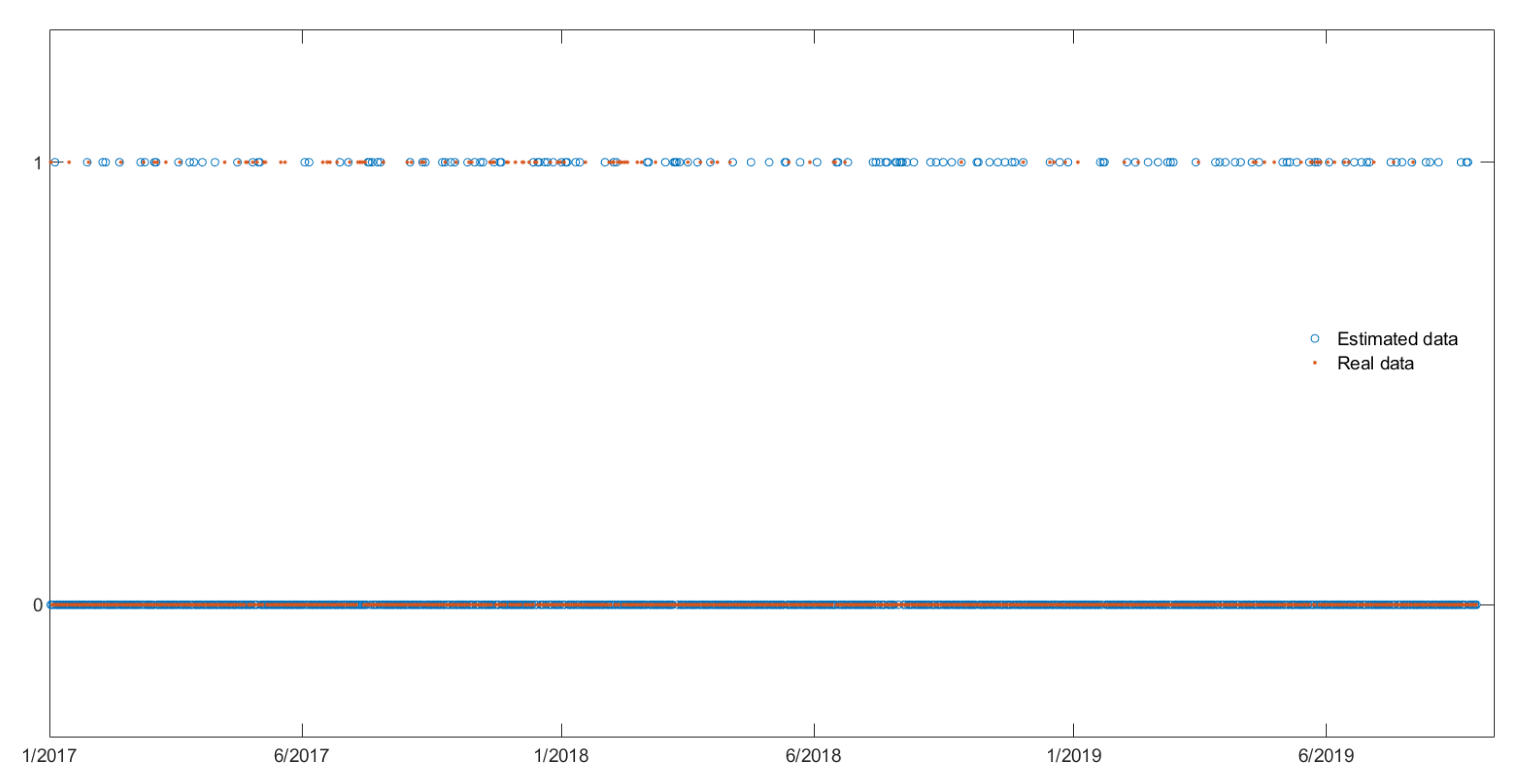
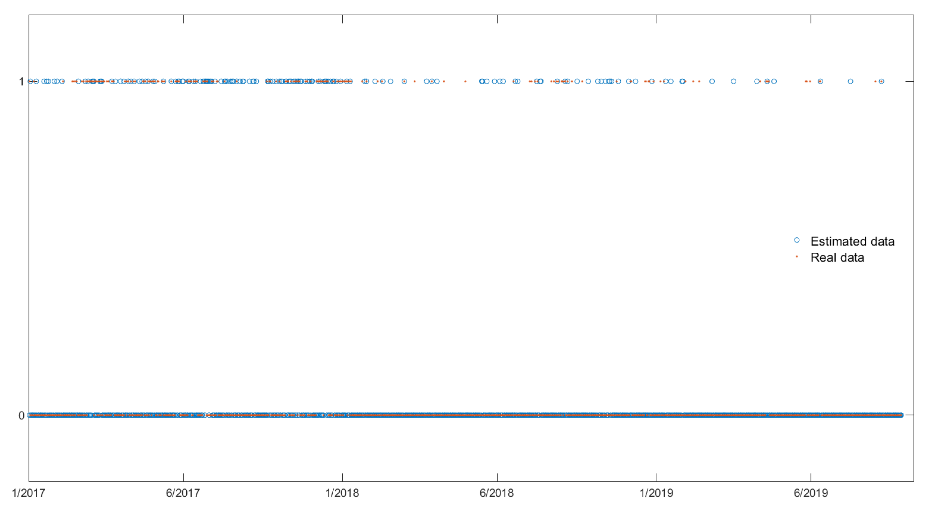
From a methodological perspective, we perform a two-layer Bayesian analysis. First, we transform the cryptocurrency series into a binary series and apply a logistic regression model on the transformed series. Specifically, if the current price return, i.e., Y t Y t 1 , exceeds a predefined threshold then we assign the value 1 and 0 otherwise. Then, we investigate whether the logistic regression model—which is widely used by applied statisticians and econometricians for analyzing binary data, see [22] and references therein—with a specific covariate set is an appropriate model for estimating the probability of observing the value 1 in these binary series. We use the methodology of Polson et al. [23] to make inference on the model’s parameters with an additional reversible jump step to allow for model uncertainty, cf. Section 2.1. Secondly, we model the log-price series data using a novel Hidden Markov (regime switching) model, namely the non-homogeneous Pólya Gamma Hidden Markov model (NHPG) of [24], cf. Section 2.2. Hidden Markov models introduce time-variation in the parameters through an underlying unobserved discrete process. In brief, at any given time t, the observed log-price data point depends on a latent (hidden) state. Hence, conditionally on the hidden states, the parameters of the data generating process vary and thus allowing for a flexible data representation. In our setting, the underlying process follows a binomial process with exogenous variables. It has been shown that the NHPG model outperforms similar models in forecasting conventional financial data, cf. [25]. Also, it uses Bayesian Model Averaging (BMA) approach for inference which has been shown to possess desirable properties for forecasting applications [26,27,28,29].
With all these in mind, the questions we aim to address are the following:
Q1.
Does the underlying information from fiat currencies, commodities, stock indices and blockchain specific variables explain/predict the probability of positive returns?
Q2.
Do the same variables have explanatory/predictive power on both the BTC and ETH cryptocurrencies?
Q3.
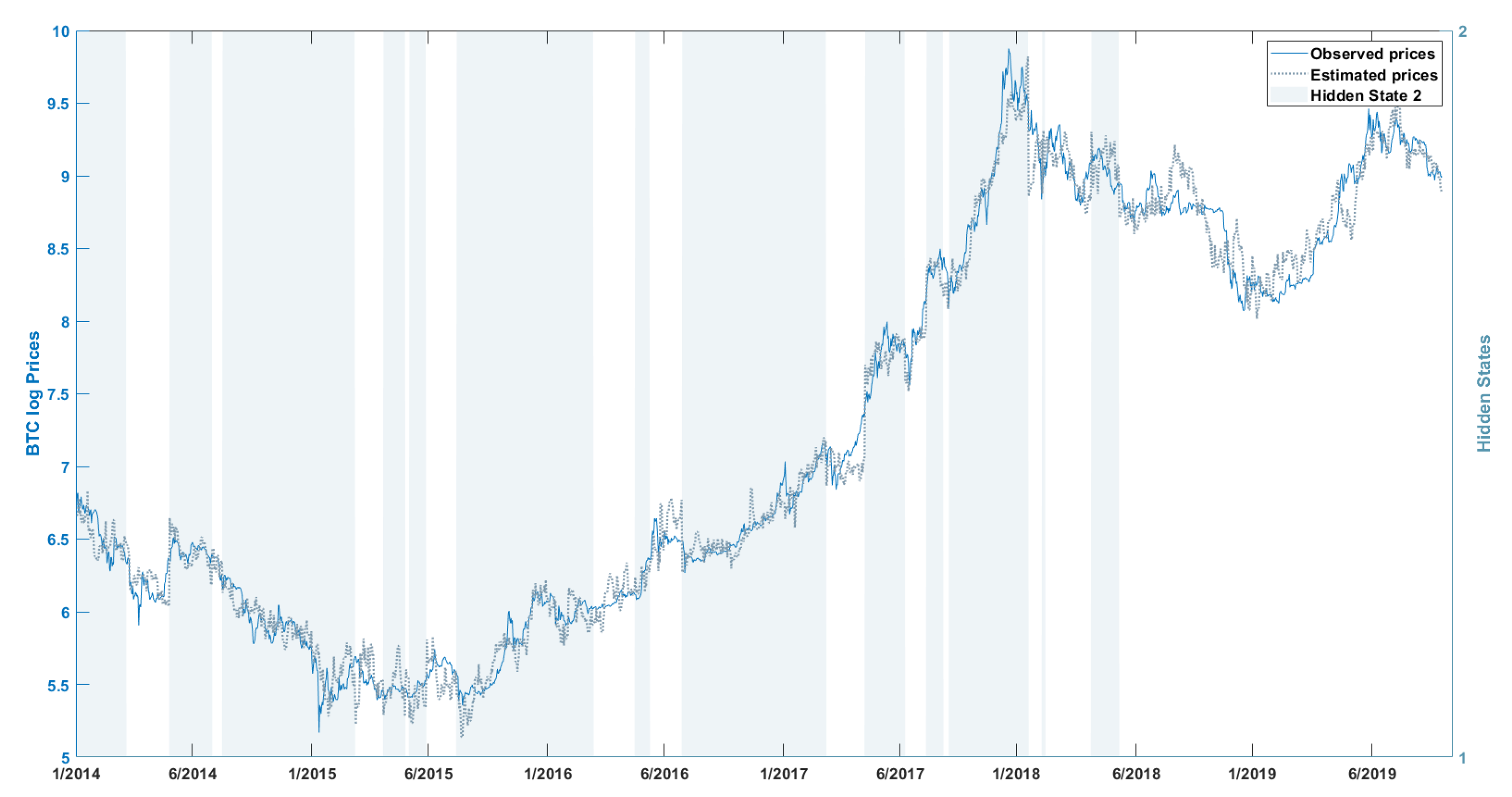
Do the same explanatory variables affect the BTC price series both on the long and short run?
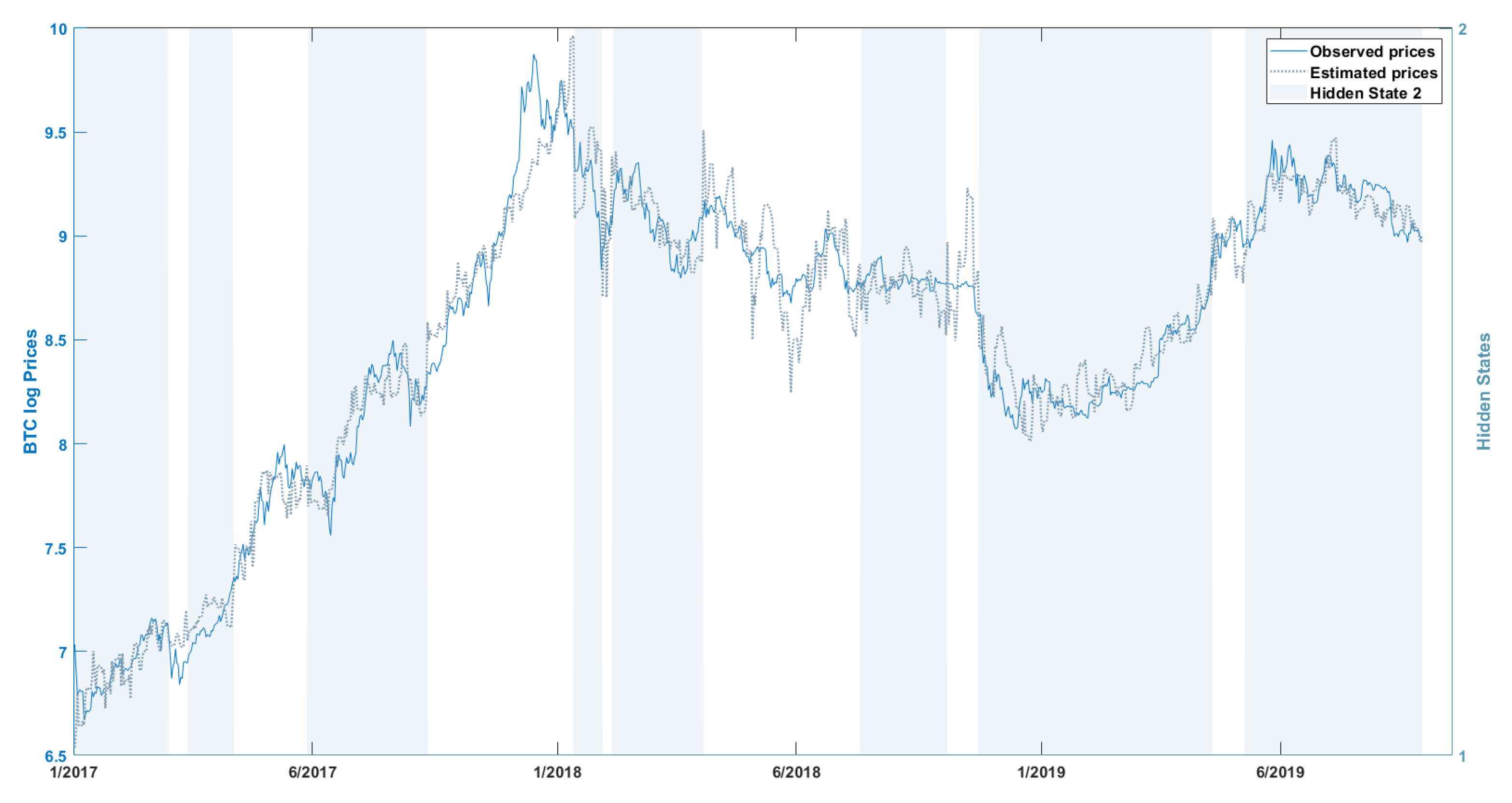
We use daily data (for both the response and the explanatory variables) between 2017 and 2019. For question Q3, we compare the BTC data of the whole 2014–2019 period to the 2017–2019 period (also used in Q1–Q2). As in most of the recent studies, we exclude the period up to 2014 which exhibits markedly different characteristics.
The findings of our experiments can be summarized as follows. The logistic model is not suitable to model the probabilities of positive daily returns of BTC and ETH. However, changing the magnitude of returns, we observe that (a) the logistic model has improved performance (b) the statistical significant covariates in the logistic regression model change and (c) the in-sample (fitting) results are different for the BTC and ETH series.
Considering the second experiment, we find that the NHPG model identifies periods of different volatility and accounts well for the heteroskedacity of all three price series (BTC short and long periods and ETH). Graphically, this is illustrated in later figures. The hidden states—which may be described as periods of high and low volatility—are not persistent, i.e., the transitions between the two states are frequent. Based on the same figures, the in-sample performance of the NHPG algorithm is good. However, the set of included predictors—predictors with posterior probability of inclusion above 0.5—is large, which implies that each predictor explains only a small fraction of the volatility of the series. Concerning specific predictors, the exclusion of some of the fiat currency exchange rates for the ETH series suggests a (still) more geographically restricted interest for the currency in comparison to BTC. It is also worth mentioning that the cryptocurrency specific variables, hash rate and average block size are not significant for modeling the BTC and ETH price series. This may indicate a more mature and stabilizing mining network that is less responsive to price expectations, sentiment or extreme speculation.
Finally, as shown in the last figure, the mean posterior out-of-sample predictions, although better for ETH than for BTC, are in general not good as they frequently even miss the direction of movement of the series. However, this is a common outcome in exchange rates [30,31]. In sum, our results confirm that the Hidden Markov approach is promising in the understanding of cryptocurrencies price formation and back earlier findings that cryptocurrencies are unlike any existing financial asset and hence that their understanding requires novel tools and ideas.
In the related literature, the first layer of our methodology, i.e., the logistic regression model, falls into the binary regression models literature. They have only been applied in the cryptocurrency context, by [32] to forecast the daily price direction of BTC, by [33] to study the price co-explosivity in leading cryptocurrencies and by [34] to study the herding behavior of BTC. As far as the second layer of our methodology, the present NHPG model falls into the Markov-switching literature that is the benchmark for predicting exchange rates, see [35] and [36,37] and explaining financial time series, see [38] and references therein. This class of models, account for the non-stationarities and non-linearities of the time series. Although standard in financial applications ([38]), Hidden Markov models have been applied in the cryptocurrency context by [39] as Markov-switching GARCH models to model the volatility dynamics of BTC, by [40], as a state-space model for representing the BTC price series, by [18] as multivariate state state-space models in forecasting cryptocurrencies, as homogeneous Hidden Markov, i.e., hidden Markov models with constant transition probabilities, by [41,42], and in the understanding of price bubbles by [43]. Also, [44], study the BTC and ETH prices under structural break setting while [45] study the cryptocurrency returns and volatility under stochastic volatility model with discontinuous jumps. The use of the NHPG model in explaining and predicting the BTC and ETH price series is also supported by the findings of various articles. For example the authors of [46,47] and [8], demonstrate the non-stationarity of the BTC index and volume and underline the importance of modeling non-linearity in Bitcoin prediction models. This is further elaborated by Beckmann and Schüssler [26] who suggest that model selection and the use of averaging criteria are necessary to avoid poor forecasting results. Following the similar reasoning, Phillip et al. [11] posit that standard models are inadequate to capture the extreme variability of cryptocurrencies and argue in favor of more composite approaches. In an important finding, Ciaian et al. [3] show that the Bitcoin price series exhibits structural breaks and identifies periods of data (prior to 2013 and between 2013 and 2015) of markedly different variance and other econometric characteristics. Their findings further suggest that significant price predictors may vary over time. Pichl and Kaizoji [48] use data from various time periods to demonstrate, among other results, that the BTC price series exhibits heteroskedasticity.
Finally, the present paper falls into the strand of literature that studies the explanatory and predictive power of traditional financial and economic indices on the cryptocurrency price series. To name a few, Refs. [4,49] analyze the relationship between BTC, gold and USD, Ref. [50] study the predictive power of a large set of exogenous variables, such as commodities, volatility indices, stock indices. Subsets of the studied indices are studied under various settings, see e.g., [7,18,40,47,48,51,52,53].
All in all, our aim is to contribute to the literature that studies the modeling and prediction of cryptocurrencies, using a novel Bayesian elaborate econometric model and to try to gain understanding in the statistical, econometric and financial properties of existing cryptocurrencies.
The rest of the paper is structured as follows. In Section 2, we describe the two econometric models of this study: the logistic regression model is described analytically in Section 2.1 and the NHPG model and simulation scheme is described in Section 2.2. The empirical study is presented in Section 3. In detail, the data set that we used is described in Section 3.1, the results regarding the logistic model are presented in Section 3.2 and lastly, the results regarding the NHPG model are presented in Section 3.3. We conclude the paper with a discussion of the limitations of the present model and directions for future work in Section 4.
This paper considerably extends its earlier conference version. Concerning the applied methodology, we provide a rigorous description of the logistic regression model for studying the probabilities of positive returns (Section 2.1) and of the NHPG model (Section 2.2). In addition, we have updated the data set—BTC and ETH series—and the covariate set. Specifically, in the covariate set, (Table 1), we have included the Russel 2000 index, excluded the autoregressive terms and applied different transformations on the variables. More importantly, concerning the results, this paper includes the novel analysis of the logistic model (Section 3.2) and based on the new covariate set, it offers more enriched outcomes and more comprehensive insight from the analysis of the NHPG model (Section 3.3).

2. Methodology

2.1. The Logistic Regression Model

Let Y t be the ETH or the BTC price series with realization y t . Also, consider a set of r 1 available predictors X t with realization x t = ( 1 , x 1 t , , x r 1 t ) at time t. The explanatory variables (predictors) X t that are used in the present analysis are described in Table 1. We transform the cryptocurrency price series as a binary series, i.e., a series that takes the values 1 or 0, as follows. Let
U t , α = I Y t Y t 1 α ,
where I denotes the indicator function that takes the value 1 if Y t Y t 1 α and 0 otherwise and α is a predefined threshold. Intuitively, we study the connection of the predictors X with the probability of having positive daily returns Y t Y t 1 α . We perform our analysis for various positive thresholds, α 0 , 1 , , 5 % .
We treat the binary series U t , α as a Bernoulli(pt) variable. From the class of the generalized linear models, we use a logit link to model the probabilities p t . The standard logistic regression model is defined as
U t , α B e r n o u l l i ( p t ) ,
p t = g 1 η t .
with η t = x t β , β the logistic regression coefficients and g ( z ) = log z 1 z the logit link function. Then, the probabilities are modeled as,
log p t 1 p t = x t β p t = exp x t β 1 + exp x t β .
We use the recently proposed latent variable scheme, namely the Pólya-Gamma data augmentation method of [23] which has significantly improved results.
The authors introduce of [23] proved that binomial likelihoods—or Bernoulli likelihoods—parametrized by log odds can be represented as mixtures of Gaussian distributions with respect to the Pólya-Gamma distribution. Their main result is that letting p ( ω ) be the density of a Pólya-Gamma latent variable ω , with ω PG ( b , 0 ) , for b > 0 , the following identity holds for all a R ,
exp ψ a 1 + exp ψ b = 2 b exp k ψ 0 exp ω ψ 2 / 2 p ω d ω ,
with k = a b / 2 . Furthermore, the conditional distribution of ω ψ is also Pólya-Gamma, PG ( b , ψ ) .
When ψ = x β , the previous identity gives rise to a conditionally conjugate augmentation scheme for Bernoulli likelihoods of logistic parameters. The likelihood is given by
L β = t = 1 N exp x t β 1 + exp x t β u t 1 1 + exp x t β 1 u t = t = 1 N exp x t β u t 1 + exp x t β .
Using the result of [23] with k t = u t 1 / 2 and setting Ω = d i a g { ω 1 , , ω T } , the augmented likelihood is proportional to
L β , ω t = 1 T 1 2 exp k t x t β 0 exp ω t , s x t β 2 / 2 p ( ω t ) d ω t .
Assuming as prior distributions ω PG ( 1 , 0 ) and β N m β 0 , V β 0 , simulation from the posterior distributions can be done iteratively in two steps:
ω t u t PG 1 , x t β , t = 1 , , T
β U , Ω N m β , V β ,
where V β = X Ω X + V β 0 1 1 and m β = V β X k + V β 0 1 m β 0 , and k = u 1 1 / 2 , , u T 1 / 2 .
To account for model uncertainty, on the predictor set, we perform a reversible jump step withing the augmented Pólya-Gamma data augmentation scheme, as proposed in [24].

Evaluation Metrics

For each iteration, we kept an in-sample replication of the binary series and compared it with the actual binary series U t . Using a 1-0 loss function, we measure the accuracy of the logistic regression model—by means of the average number of misestimated data values per iteration—in representing the studied series. We report the results of this study in Section 3.2.

2.2. The Non-Homogeneous Polya-Gamma Hidden Markov Model

Given a time horizon T 0 and discrete observation times t = 1 , 2 , , T , we consider an observed random process Y t t T and a hidden underlying process Z t t T . The hidden process Z t is assumed to be a two-state non-homogeneous discrete-time Markov chain, s = 1 , 2 , that determines the states of the observed process. In our setting, the observed process is either the BTC or the ETH logarithmic prices series. The description of the hidden states is not pre-determined and is subject to the interpretation of the results.
Let y t and z t be the realizations of the random processes Y t and { Z t } , respectively. We assume that at time t , t = 1 , , T , y t depends on the current state z t and not on the previous states. Consider also the set of predictors X t of Section 2.1. A subset of the predictors X t ( 1 ) X t of length r 1 1 affects the cryptocurrency linearly. In addition, a subset X t ( 2 ) { X t } of length r 2 1 is used to describe the dynamics of the time-varying transition probabilities, i.e., the probabilities of moving from hidden state s = 1 to the hidden state s = 2 and vice versa. Thus, we allow the predictors to affect the series { Y t } linearly and non-linearly. Given the above, the cryptocurrency price series Y t can be modeled as
Y t Z t = s N ( x t 1 ( 1 ) B s , σ s 2 ) , s = 1 , 2 ,
where B s = ( b 0 s , b 1 s , , b r 1 1 s ) are the regression coefficients and N ( μ , σ 2 ) denotes the normal distribution with mean μ and variance σ 2 . The dependence of the observed process on the unobserved states, allows the model to capture the non-stationarities, non-linearities and the changes in the volatility, i.e., heteroskedasticity of the cryptocurrency series.
The dynamics of the unobserved process Z t can be described by the time-varying (non-homogeneous) transition probabilities, which depend on the predictors X t ( 2 ) and are given by the following relationship
P ( Z t + 1 = j Z t = i ) = p i j ( t ) = exp ( x t ( 2 ) β i j ) j = 1 2 exp ( x t ( 2 ) β i j ) , i , j = 1 , 2 ,
where β i j = ( β 0 , i j , β 1 , i j , , β r 2 1 , i j ) is the vector of the logistic regression coefficients to be estimated. Please note that for identifiability reasons, we adopt the convention of setting, for each row of the transition matrix, one of the β i j to be a vector of zeros. Without loss of generality, we set β i j = β j i = 0 for i , j = 1 , 2 , i j . Hence, for β i : = β i i , i = 1 , 2 , the probabilities can be written in a simpler form
p i i ( t ) = exp ( x t ( 2 ) β i ) 1 + exp ( x t ( 2 ) β i ) and p i j ( t ) = 1 p i i ( t ) , i , j = 1 , 2 , i j .
Summing up, the unknown quantities of the NHPG are θ s = B s , σ s 2 , β s , s = 1 , 2 , i.e., the parameters in the mean predictive regression equation and the parameters in the logistic regression equation for the transition probabilities of the unobserved process Z t , t = 1 , , T . We follow the Bayesian methodology of [24], for joint inference on model specification, model parameters and predictions. Specifically, the authors in [24] use conditional conjugate analysis for the parameters in the mean predictive regression equation, i.e.
σ s 2 IG ( p , q ) , B s , σ s 2 N ( L 0 , σ s 2 V 0 ) , s = 1 , 2 ,
where IG denotes the Inverted-Gamma distribution. The conditional and the marginal posterior distributions for the state specific parameters σ s and B s ,
σ s 2 IG p + n s 2 , q + 1 2 L 0 s V 0 s 1 L 0 s + Y s Y s L s V s 1 L s ,
B s σ s 2 , z T , y T N L s , σ s 2 V s ,
with V s = V 0 s 1 + X s ( 1 ) X s ( 1 ) 1 , L s = V s V 0 s 1 L 0 s + X s ( 1 ) Y s . To make inference about the logistic regression coefficients, the authors model the probabilities of staying at the same state for two consecutive time periods, i.e., p s s t . They define, for t = 1 , T 1 , the quantity Z ˜ t + 1 s = I Z t + 1 = Z t = s with the sum t Z ˜ t + 1 s , be the number of times that the chain was at state s for two consecutive time periods. Then,
p Z ˜ t + 1 s = 1 x t ( 2 ) = p s s t = exp x t ( 2 ) β s 1 + exp x t ( 2 ) β s l o g i t p s s ( t ) = x t ( 2 ) β s , s = 1 , 2 ,
and inference for the probabilities falls to the case of the logistic model of Section 2.1.
Finally, for every dataset we kept L out-of-sample observations and compare the estimated forecasts using the NHPG model. Given model M, the predictive distribution of y T + L , L 1 is
f p y T + L y T + L 1 = f y T + L y T + L 1 , z T + L 1 , M , β M , θ M π β M , θ M y T + L 1 d β M d θ M ,
where f y T + 1 y T , z T , β M , θ M = s = 1 2 P Z T + 1 = s Z T = z T f s y T + 1 .
All in all, the MCMC sampling scheme is constructed with recursive updates of (i) the latent variables z T given the current value of the model parameters by using the scaled Forward–Backward algorithm (Scott [54]) (ii) the logistic regression coefficients by adopting the auxiliary variables method of Polson et al. [23] given the sequence of states z T , (iii) the mean regression coefficients conditional on z T by using the Gibbs sampling algorithm (iv) the covariate set using a couple of reversible jump steps and (v) the predictive distributions given the parameters and hidden states. The MCMC steps are detailed in Algorithm 1.
Algorithm 1 MCMC Sampling Scheme for Inference on Model Specification and Parameters
1:
% After each procedure the parameters and model space are updated conditionally on the previous quantities
2:
procedureScaled Forward–Backward( θ , y t )
3:
%Simulation of a realization of the hidden states z t
4:
for t = 1 , , T and i = 1 , 2 do
5:
   π t i θ α t ( s ) j = 1 2 α t j = P z t = i θ , y t Simulation of the scaled forward probabilities
6:
for t = T , T 1 , , 1 do
7:
   z t P z t z t + 1 = p i z t + 1 π t i θ j = 1 m p j z t + 1 π t j θ          Backwards simulation of z t
8:
procedureMean_Regres_Param( β s , σ s , s = 1 , 2 )
9:
%Simulation of the mean regression parameters
10:
for s = 1 , 2 do                Conjugate analysis with Gibbs sampler
11:
   β σ 2 f B , σ 2 I G            f B Normal and f σ Inverse-Gamma
12:
procedureLog_Regres_Coef( β s , ω s )
13:
%Simulation of the logistic regression coefficients
14:
for s = 1 , 2 do               Pólya-Gamma data augmentation scheme
15:
  augment the model space with ω s      Conjugate analysis on the augmented space
16:
  sample from β s f β s ω
17:
    and ω s β s PG      Posteriors f β s ω Normal and PG Pólya-Gamma
18:
procedureDouble_Rev_Jump( X ( 1 ) , X ( 2 ) )
19:
%Variable selection with double reversible jump step
20:
for i = 1 , 2 do %Propose to add/remove a covariate
21:
  add: choose X c a n d i d a t e from X X ( i ) c        Calculate acceptance probability α
22:
  if α < r a n d ( 0 , 1 ) then X ( i ) X ( i ) X c a n
23:
  remove: choose X c a n d i d a t e from X ( i )         Calculate acceptance probability α
24:
  if α < r a n d ( 0 , 1 ) then X ( i ) X ( i ) X c a n c
25:
procedurePredict
26:
% Make L-steps-ahead predictions
27:
for t = T + 1 , , T + L do
28:
   y ^ t f with f y T + 1 y T , z T , β M , θ M = s = 1 2 P Z T + 1 = s Z T = z T f s y T + 1 .

3. The Empirical Application

3.1. The Data

We assess the explanatory power of 12 financial/economic and 2 cryptocurrency specific variables, outlined in Table 1, on the BTC and ETH series, through two different experimental exercises: (a) the logistic regression model and (b) NHPG model. We analyze the daily BTC and ETH price series for the period ranging from 1 / 1 / 2017 to 16 / 11 / 2019 . Missing data due to the non-business days are filled with the last available value. For the first exercise, we transform the price series into binary series using the transformation Y t Y t 1 α .
Table 1. List of explanatory variables along with the applied transformations and the online resources. The Hash Rate (HR) and Average Block Size (AVS) have been retrieved [55] for Bitcoin and from [56] for Ether.
Explanatory Variables
DescriptionSymbolTransformationRetrieved from
US dollars to Euros exchange rateUSD/EURNormalizedinvesting.com
US dollars to GBP exchange rateUSD/GBPNormalizedinvesting.com
US dollars to Japanese Yen exchange rateUSD/JPYNormalizedinvesting.com
US dollars to Chinese Yuan exchange rateUSD/CNYNormalizedinvesting.com
Russel 2000 indexR2000Normalizedfinance.yahoo.com
Standard & Poor’s 500 indexSP500Normalizedfinance.yahoo.com
NASDAQ Composite indexNASDAQNormalizedfinance.yahoo.com
Dow Jones Industrial AverageDOWNormalizedfinance.yahoo.com
Crude Oil Futures priceOILNormalizedfinance.yahoo.com
Price of GoldGOLDNormalizedfinance.yahoo.com
CBOE Volatility indexVIXNormalizedfinance.yahoo.com
Equity market Economic Uncertainty indexEUINonefred.stlouisfed.org
Hash RateHRPercentage of changequandl.com/etherscan.io
Average Block SizeAVSPercentage of changequandl.com/etherscan.io
The aim of this experiment is to model/explain the probability of a positive return. We repeat the experiment for different magnitudes ( α ) of returns, i.e., gains more than 0 % , 1 % , , 5 % . For the second exercise, we use the logarithm of the price series of the two aforementioned cryptocurrencies. Additionally to the previous data sets, we apply the NHPG methodology in a larger BTC log-price series (for the period ranging from 1/1/2014 until 16/11/2019). The closing BTC prices were downloaded from [20] and the ETH prices were downloaded from [56].
Table 2. Correlation matrix of the explanatory variables.
VariablesUSD/EURUSD/GBPUSD/JPYUSD/CNYR2000SP500NASDAQDOWOILGOLDVIXEUIHRAVS
USD/EUR1.00.630.60.540.160.250.260.2−0.82−0.330.080.130.01−0.02
USD/GBP0.631.00.92−0.070.660.730.730.71−0.56−0.18−0.090.18−0.01−0.02
USD/JPY0.60.921.0−0.090.550.660.650.64−0.54−0.31−0.030.230.00−0.01
USD/CNY0.54−0.07−0.081.0−0.06−0.08−0.06−0.1−0.42−0.210.12−0.050.00−0.02
R20000.160.660.55−0.061.00.950.950.95−0.08−0.07−0.230.03−0.02−0.01
SP5000.250.730.66−0.080.951.01.00.95−0.25−0.19−0.110.12−0.02−0.02
NASDAQ0.260.730.65−0.060.950.951.00.99−0.25−0.18−0.070.13−0.02−0.01
DOW0.20.710.64−0.10.951.00.991.0−0.2−0.16−0.090.12−0.02−0.02
OIL−0.82−0.56−0.54−0.42−0.08−0.25−0.25−0.21.00.6−0.21−0.18−0.000.00
GOLD−0.33−0.18−0.31−0.21−0.07−0.19−0.18−0.160.61.0−0.12−0.09−0.000.00
VIX0.08−0.09−0.030.12−0.23−0.11−0.07−0.09−0.21−0.121.00.390.020.00
EUI0.130.180.23−0.050.030.120.130.12−0.18−0.090.391.0−0.02−0.01
HR0.01−0.010.000.00−0.02−0.02−0.02−0.020.00−0.010.02−0.021.0−0.18
AVS−0.02−0.02−0.01−0.02−0.01−0.02−0.01−0.020.020.010.00−0.01−0.181.0

3.2. Results: The Logistic Regression Model

We report the in-sample performance for the logistic regression model in Table 3 for every threshold and for both cryptocurrencies. Even though the in-sample performance—based on the large number of incorrect point estimates of the series—is poor, we see that when the threshold α increases, the in-sample performance is improved.
To be more precise, we find that for α = 0 % the covariate set has no explanatory power on the U t , α since the probability of incorrect estimations is almost 50 % for both coins. However, for α = 5 % the probability of incorrect estimations drops to 17 % for the binary BTC series and to 25.5 % for the binary ETH series. This result is an indication that the accounted covariate set, which includes fiat currencies, stock indices and commodities can be used to explain/predict the possibility of larger positive returns. A visualization of the best in-sample performance for the U t , 5 series for BTC and ETH is in Figure 1 and Figure 2.
In Table 4 and Table 5, we report the posterior probabilities of inclusion π k , k = 1 , , K of the K explanatory variables for the studied logistic models for the BTC and ETH binary series, respectively. For both coins, we observe that the studied covariated set does not affect nor predict the probability of positive return, i.e., Y t Y t 1 0 .
However, if we change the magnitude of return ( α ), we find that there is a correlation between the covariate set and the probabilities of observing Y t Y t 1 α , α = 1 , 2 , 3 , 4 , 5 % . We find that the sets including the covariates that affect the binary BTC and ETH series—covariates with posterior probability of inclusion above 0.5—are different. Also, we observe that even though the binary ETH series is correlated with more covariates than the covariates of the binary BTC series, the logistic model has worse performance in explaining the studied series (as seen in Table 3).
The results of this experiment imply that the accounted covariate set has some explanatory power on the series but a more elaborated and more complicated model, such as the NHPG model, needs to be considered.

3.3. Results: The NHPG Model

In this section, we present the results of the NHPG model using the logarithmic ETH and BTC price series. Figure 3, Figure 4 and Figure 5 plot the log ETH, log BTC and extended log BTC datasets (blue line) along with the estimated in-sample time series (gray line). This shows graphically the good in-sample performance of the NHPG model to replicate the log BTC and log ETH series. Shaded bars indicate the time periods that the underlying hidden process is in state 1. The states alternate between 1 and 2 rather frequently, confirming previous studies on the heteroskedasticity of the series, see e.g., [11], and on the existence of structural breaks and regime switches, see e.g., [39,44].
However, the out-of-sample performance of the NHPG is poor. Figure 6, shows the posterior mean (gray lines), of the 30 empirical predictive distributions, along with the actual out-of sample log prices of ETH, BTC (blue line). The mean posterior out-of-sample predictions are in general not good, as they frequently miss the direction of movement of the series.
Even worse, when we examine the posterior prediction intervals with boundaries the 2.5 % and 97.5 % quantiles of the empirical predictive densities—instead of the mean point forecasts—we find, for some cases, that they do not include the actual out-of-sample values. Hence, we confirm the claim of previous studies that financial and economic variables do not accurately predict the price fluctuation of cryptocurrencies. The good in-sample and poor out-of-sample performance of the two-state Non-Homogeneous Hidden Markov models is also observed in the exchange rate literature, see for example [30,31].
In Table 6, we report the posterior probabilities of inclusion of the explanatory variables for the mean equation—first number—and the logistic regression—second number in every cell. Variables with posterior probability of inclusion above 0.5 in either the mean equation or the transition probabilities are marked with bold. These variables make up the median probability model (MPM). Although the BTC and ETH are correlated [15], the variables that affect the series (by means of the MPM) are not the same. The MPM of ETH consists of 7 covariates: the USD/EUR, USD/GBP and USD/CNY exchange rates, Russel 2000, S&P 500, Dow Jones, NASDAQ indices. The MPM of BTC additionally contains the USD/JPY exchange rate and VIX. This difference on the exchange rates indicates that ETH is more geographically restricted. Moreover, the hash rate (HR) and Average Block size is insignificant for both cryptocurrencies. Regarding the extended BTC dataset, we find that Gold and Crude Oil future prices are also significant. Furthermore, it is worth mentioning that all the effects are linear in BTC series and hence the transition probabilities of hidden states are homogeneous (constant through time). This is in difference with ETH price series where S&P 500 and USD/GBP affects the series also non-linearly. The inclusion of these two variables in the transition probabilities equation results to the non-constant transition probabilities and consequently indicates that the Non-Homogeneous Hidden Markov model is promising in the understanding of cryptocurrencies price formation. The non-constant transition probabilities along with the fact that there exist other variables with non-negligible posterior probabilities of inclusion (above 0.3), imply that the are other drives that drive changes in the underlying process that go beyond the financial aspects that have been considered in the present setting. Finally, we observe that even though the number of statistical important variables is large, for both coins, the forecasting performance of this model is very modest. This is an indication that non-traditional financial and economic variables need to be considered.
To sum up, even though we observe a large number of statistical significant explanatory variables, the insufficient forecasting performance of the NHPG model confirms that the cryptocurrencies are still decoupled from the mainstream financial and economic assets [57].

4. Concluding Remarks

We applied a logistic regression model with a predefined covariate set to model the probabilities of observing daily returns exceeding a predefined threshold for the Bitcoin (BTC) and Ether (ETH) series. We show empirically that the logistic model has weak fitting performance. However, we find that changing the magnitude of positive returns, improves the fitting performance of the logistic regression model. This result motivated us to incorporate the logistic regression model into a more complex model. Therefore, we applied a specific instance of the Non-Homogeneous Hidden Markov models to the logarithm of BTC and ETH price series.
We used the non-homogeneous Pólya-Gamma Hidden Markov Model (NHPG) of [24]. Focusing on a data set of financial/economic predictors, we studied general properties of the cryptocurrency price series. While the NHPG algorithm exhibited good in-sample performance, it revealed that changes in the underlying two-state Markov process are frequent, thus indicating that the states are not persistent, contributing to the already high heteroskedasticity of both the Bitcoin and the Ether data series. Notably, both cryptocurrency specific variables were not found significant for BTC and ETH. Significance of exchange rates revealed a more geographically restricted interest for ETH than for BTC.
From a modeling point of view, the median probability model included too many covariates, thus, indicating data with high variability and confirming that financial and economic variables—even if cryptocurrency specific—are not enough to explain the formation of cryptocurrency prices. Along with the poor out-of-sample predictions, these findings show that even algorithms with good performance on conventional financial data do not capture all aspects of cryptocurrencies. In the main takeaway of this study, these results back earlier findings that cryptocurrencies are unlike any other financial asset and that the understanding of their properties requires not only the combination of more sophisticated models but also the inception of novel ideas and tools.
While the current study offers a novel perspective on the hidden states—and hence on the underlying forces—that drive cryptocurrency markets, it also suggests that the analysis of their price formation requires more elaborate tools. Recent advances in deep neural networks provide methods to identify hidden layers that approximate complex non-linear relationships. Specifically, by exploring electronic high-frequency data of supply, demand and prices in financial markets, Deep Learning models can uncover universal price formation mechanisms, [58]. This approach seems particularly promising for cryptocurrency markets. Along these lines, the current model may prompt a more extensive application of the rich Hidden Markov theory and analytical toolbox on cryptocurrency markets.
All in all, the investigation of the exogenous variables that affect or drive the cryptocurrency market can be useful to investors, policy makers, traders for portfolio allocation, risk management and trading strategies.

Author Contributions

Conceptualization, C.K.,S.L., G.P. ; methodology, C.K. and S.L.; software, C.K.; validation, C.K. and S.L.; formal analysis, C.K.; investigation, C.K.; resources, C.K.; data curation, C.K. and S.L.; writing–original draft preparation, C.K.; writing–review and editing, C.K. and S.L.; visualization, C.K and S.L.; supervision, G.P.; project administration, G.P.; funding acquisition, G.P. All authors have read and agreed to the published version of the manuscript.

Funding

Stefanos Leonardos and Georgios Piliouras were supported by MOE AcRF Tier 2 Grant 2016-T2-1-170 and in part by the National Research Foundation (NRF), Prime Minister’s Office, Singapore, under its National Cybersecurity R&D Program (Award No. NRF2016NCR-NCR002-028) and administered by the National Cybersecurity R&D Directorate. Georgios Piliouras acknowledges SUTD grant SRG ESD 2015 097 and NRF 2018 Fellowship NRF-NRFF2018-07.

Conflicts of Interest

The authors declare no conflict of interest. The funders had no role in the design of the study; in the collection, analyses, or interpretation of data; in the writing of the manuscript, or in the decision to publish the results.

References

  1. Cheah, E.T.; Fry, J. Speculative bubbles in Bitcoin markets? An empirical investigation into the fundamental value of Bitcoin. Econ. Lett. 2015, 130, 32–36. [Google Scholar] [CrossRef] [Green Version]
  2. Klein, T.; Thu, H.; Walther, T. Bitcoin is not the New Gold – A comparison of volatility, correlation, and portfolio performance. Int. Rev. Financ. Anal. 2018, 59, 105–116. [Google Scholar] [CrossRef]
  3. Ciaian, P.; Rajcaniova, M.; Kancs, A. The economics of BitCoin price formation. Appl. Econ. 2016, 48, 1799–1815. [Google Scholar] [CrossRef] [Green Version]
  4. Dyhrberg, A.H. Bitcoin, gold and the dollar – A GARCH volatility analysis. Financ. Res. Lett. 2016, 16, 85–92. [Google Scholar] [CrossRef] [Green Version]
  5. Bouri, E.; Gupta, R.; Tiwari, A.K.; Roubaud, D. Does Bitcoin hedge global uncertainty? Evidence from wavelet-based quantile-in-quantile regressions. Financ. Res. Lett. 2017, 23, 87–95. [Google Scholar] [CrossRef] [Green Version]
  6. Bouri, E.; Azzi, G.; Dyhrberg, A.H. On the return-volatility relationship in the Bitcoin market around the price crash of 2013. Econ. Open Access Open Assess. J. 2017, 11, 1–16. [Google Scholar] [CrossRef] [Green Version]
  7. Bouri, E.; Molnár, P.; Azzi, G.; Roubaud, D.; Hagfors, L.I. On the hedge and safe haven properties of Bitcoin: Is it really more than a diversifier? Financ. Res. Lett. 2017, 20, 192–198. [Google Scholar] [CrossRef]
  8. Demir, E.; Gozgor, G.; Lau, C.M.; Vigne, S.A. Does economic policy uncertainty predict the Bitcoin returns? An empirical investigation. Financ. Res. Lett. 2018, 26, 145–149. [Google Scholar] [CrossRef] [Green Version]
  9. Katsiampa, P. Volatility estimation for Bitcoin: A comparison of GARCH models. Econ. Lett. 2017, 158, 3–6. [Google Scholar] [CrossRef] [Green Version]
  10. Hayes, A.S. Cryptocurrency value formation: An empirical study leading to a cost of production model for valuing bitcoin. Telemat. Inform. 2017, 34, 1308–1321. [Google Scholar] [CrossRef]
  11. Phillip, A.; Chan, J.; Peiris, S. On generalized bivariate student-t Gegenbauer long memory stochastic volatility models with leverage: Bayesian forecasting of cryptocurrencies with a focus on Bitcoin. Econom. Stat. 2018. [Google Scholar] [CrossRef]
  12. Georgoula, I.; Pournarakis, D.; Bilanakos, C.; Sotiropoulos, D.; Giaglis, G.M. Using Time-Series and Sentiment Analysis to Detect the Determinants of Bitcoin Prices. In Proceedings of the 9th Mediterranean Conference on Information Systems, Samos, Greece, 3–5 October 2015. [Google Scholar] [CrossRef] [Green Version]
  13. Kraaijeveld, O.; Smedt, J.D. The predictive power of public Twitter sentiment for forecasting cryptocurrency prices. J. Int. Financ. Mark. Inst. Money 2020. [Google Scholar] [CrossRef]
  14. Buterin, V.; Reijsbergen, D.; Leonardos, S.; Piliouras, G. Incentives in Ethereum’s Hybrid Casper Protocol. In Proceedings of the 2019 IEEE International Conference on Blockchain and Cryptocurrency (ICBC), Seoul, Korea, 15–17 May 2019; pp. 236–244. [Google Scholar] [CrossRef] [Green Version]
  15. Borri, N. Conditional tail-risk in cryptocurrency markets. J. Empir. Financ. 2019, 50, 1–19. [Google Scholar] [CrossRef]
  16. Vora, R. Ethereum Price Analysis: Ethereum (ETH) Needs to Discover the Magic Spell to Surge on Its Own. Available online: https://www.cryptonewsz.com/ethereum-price-analysis-ethereum-eth-needs-to-discover-the-magic-spell-to-surge-on-its-own/29402/ (accessed on 27 July 2019).
  17. Gandal, N.; Halaburda, H. Can We Predict the Winner in a Market with Network Effects? Competition in Cryptocurrency Market. Games 2016, 7, 16. [Google Scholar] [CrossRef] [Green Version]
  18. Hotz-Behofsits, C.; Huber, F.; Zörner, T.O. Predicting crypto-currencies using sparse non-Gaussian state space models. J. Forecast. 2018, 37, 627–640. [Google Scholar] [CrossRef]
  19. Buterin, V. A Next-Generation Smart Contract and Decentralized Application Platform. 2014. Available online: https://github.com/ethereum/wiki/wiki/White-Paper (accessed on 1 September 2019).
  20. Crypto.com. Available online: https://coinmarketcap.com/all/views/all/ (accessed on 30 July 2019).
  21. Ethereum Foundation. Available online: https://www.ethereum.org/ (accessed on 30 July 2019).
  22. Frühwirth-Schnatter, S.; Frühwirth, R. Auxiliary mixture sampling with applications to logistic models. Comput. Stat. Data Anal. 2007, 51, 3509–3528. [Google Scholar] [CrossRef]
  23. Polson, N.G.; Scott, J.G.; Windle, J. Bayesian Inference for Logistic Models Using Polya-Gamma Latent Variables. J. Am. Stat. Assoc. 2013, 108, 1339–1349. [Google Scholar] [CrossRef] [Green Version]
  24. Koki, C.; Meligkotsidou, L.; Vrontos, I. Forecasting under model uncertainty: Non-homogeneous hidden Markov models with Pòlya-Gamma data augmentation. J. Forecast. 2018. [Google Scholar] [CrossRef] [Green Version]
  25. Meligkotsidou, L.; Dellaportas, P. Forecasting with non-homogeneous hidden Markov models. Stat. Comput. 2011, 21, 439–449. [Google Scholar] [CrossRef] [Green Version]
  26. Beckmann, J.; Schüssler, R. Forecasting exchange rates under parameter and model uncertainty. J. Int. Money Financ. 2016, 60, 267–288. [Google Scholar] [CrossRef]
  27. Groen, J.J.J.; Paap, R.; Ravazzolo, F. Real-Time Inflation Forecasting in a Changing World. J. Bus. Econ. Stat. 2013, 31, 29–44. [Google Scholar] [CrossRef] [Green Version]
  28. Wright, J.H. Forecasting US inflation by Bayesian model averaging. J. Forecast. 2009, 28, 131–144. [Google Scholar] [CrossRef] [Green Version]
  29. Wright, J.H. Bayesian Model Averaging and exchange rate forecasts. J. Econom. 2008, 146, 329–341. [Google Scholar] [CrossRef] [Green Version]
  30. Yuan, C. Forecasting exchange rates: The multi-state Markov-switching model with smoothing. Int. Rev. Econo. Financ. 2011, 20, 342–362. [Google Scholar] [CrossRef]
  31. Marsh, I.W. High-frequency Markov switching models in the foreign exchange market. J. Forecast. 2000, 19, 123–134. [Google Scholar] [CrossRef]
  32. Atsalakis, G.S.; Atsalaki, I.G.; Pasiouras, F.; Zopounidis, C. Bitcoin price forecasting with neuro-fuzzy techniques. Eur. J. Oper. Res. 2019, 276, 770–780. [Google Scholar] [CrossRef]
  33. Bouri, E.; Shahzad, S.J.H.; Roubaud, D. Co-explosivity in the cryptocurrency market. Financ. Res. Lett. 2019, 29, 178–183. [Google Scholar] [CrossRef]
  34. Bouri, E.; Gupta, R.; Roubaud, D. Herding behaviour in cryptocurrencies. Financ. Res. Lett. 2019, 29, 216–221. [Google Scholar] [CrossRef]
  35. Engel, C. Can the Markov switching model forecast exchange rates? J. Int. Econ. 1994, 36, 151–165. [Google Scholar] [CrossRef] [Green Version]
  36. Lee, H.Y.; Chen, S.L. Why use Markov-switching models in exchange rate prediction? Econ. Model. 2006, 23, 662–668. [Google Scholar] [CrossRef]
  37. Frömmel, M.; MacDonald, R.; Menkhoff, L. Markov switching regimes in a monetary exchange rate model. Econ. Model. 2005, 22, 485–502. [Google Scholar] [CrossRef] [Green Version]
  38. Mamon, R.; Elliott, R. (Eds.) Hidden Markov Models in Finance: Further Developments and Applications; Springer: Berlin/Heidelberg, Germany, 2014; Volume II. [Google Scholar]
  39. Ardia, D.; Bluteau, K.; Rüede, M. Regime changes in Bitcoin GARCH volatility dynamics. Financ. Res. Lett. 2019, 29, 266–271. [Google Scholar] [CrossRef]
  40. Poyser, O. Exploring the dynamics of Bitcoin’s price: A Bayesian structural time series approach. Eurasia. Econ. Rev. 2019, 9, 29–60. [Google Scholar] [CrossRef]
  41. Koutmos, D. Market risk and Bitcoin returns. Ann. Oper. Res. 2019. [Google Scholar] [CrossRef]
  42. Koutmos, D. Liquidity uncertainty and Bitcoin’s market microstructure. Econ. Lett. 2018, 172, 97–101. [Google Scholar] [CrossRef]
  43. Phillips, R.C.; Gorse, D. Predicting cryptocurrency price bubbles using social media data and epidemic modelling. In Proceedings of the 2017 IEEE Symposium Series on Computational Intelligence (SSCI), Honolulu, HI, USA, 27 November–1 December 2017. [Google Scholar] [CrossRef] [Green Version]
  44. Mensi, W.; Al-Yahyaee, K.H.; Kang, S.H. Structural breaks and double long memory of cryptocurrency prices: A comparative analysis from Bitcoin and Ethereum. Financ. Res. Lett. 2019, 29, 222–230. [Google Scholar] [CrossRef]
  45. Chaim, P.; Laurini, M.P. Volatility and return jumps in Bitcoin. Econ. Lett. 2018, 173, 158–163. [Google Scholar] [CrossRef]
  46. Balcilar, M.; Bouri, E.; Gupta, R.; Roubaud, D. Can volume predict Bitcoin returns and volatility? A quantiles-based approach. Econ. Model. 2017, 64, 74–81. [Google Scholar] [CrossRef] [Green Version]
  47. Jang, H.; Lee, J. An Empirical Study on Modeling and Prediction of Bitcoin Prices With Bayesian Neural Networks Based on Blockchain Information. IEEE Access 2018, 6, 5427–5437. [Google Scholar] [CrossRef]
  48. Pichl, L.; Kaizoji, T. Volatility Analysis of Bitcoin Price Time Series. Quant. Financ. Econ. 2017, 1, 474–485. [Google Scholar] [CrossRef]
  49. Baur, D.G.; Dimpfl, T.; Kuck, K. Bitcoin, gold and the US dollar—A replication and extension. Financ. Res. Lett. 2018, 25, 103–110. [Google Scholar] [CrossRef]
  50. Walther, T.; Klein, T.; Bouri, E. Exogenous drivers of Bitcoin and Cryptocurrency volatility—A mixed data sampling approach to forecasting. J. Int. Financ. Mark. Inst. Money 2019, 63, 101133. [Google Scholar] [CrossRef]
  51. Van Wijk, D. What Can Be Expected from the BitCoin. Ph.D. Thesis, Erasmus Universiteit Rotterdam, Rotterdam, The Netherlands, 2013. [Google Scholar]
  52. Yermack, D. Chapter 2–Is Bitcoin a Real Currency? An Economic Appraisal. In Handbook of Digital Currency; Chuen, D.L., Ed.; Academic Press: San Diego, CA, USA, 2015; pp. 31–43. [Google Scholar] [CrossRef]
  53. Estrada, J.C.S. Analyzing Bitcoin Price Volatility. Ph.D. Thesis, University of California, Berkeley, CA, USA, 2017. [Google Scholar]
  54. Scott, S.L. Bayesian Methods for Hidden Markov Models. J. Am. Stat. Assoc. 2002, 97, 337–351. [Google Scholar] [CrossRef]
  55. Quantl.com. The World’S Most Powerful Data Lives on Quandl. Available online: https://www.quandl.com/ (accessed on 30 July 2019).
  56. Etherscan.io. Available online: https://etherscan.io (accessed on 30 July 2019).
  57. Gil-Alana, L.A.; Abakah, E.J.A.; Rojo, M.F.R. Cryptocurrencies and stock market indices. Are they related? Res. Int. Bus. Financ. 2020, 51, 101063. [Google Scholar] [CrossRef]
  58. Sirignano, J.; Cont, R. Universal features of price formation in financial markets: Perspectives from deep learning. Quant. Financ. 2019, 19, 1449–1459. [Google Scholar] [CrossRef]
Figure 1. Realization of the binary BTC series with α = 5 % using the logistic regression model. The blue circles represent the realized series whereas the red dots are the actual data points.
Futureinternet 12 00059 g001
Figure 2. Realization of the binary ETH series with α = 5 % using the logistic regression model. The blue circles represent the realized series whereas the red dots are the actual data points.
Futureinternet 12 00059 g002
Figure 3. Logarithmic ETH price series (blue line) and in-sample estimated logarithmic ETH price series for the period 6/2016–5/2019 (gray dotted line). Shaded bars mark times with hidden state 1 (smoothed probability above 0.5). The model accounts for the heteroskedasticity of the series.
Futureinternet 12 00059 g003
Figure 4. Logarithmic BTC prices series (blue line) and in-sample estimated logarithmic BTC price series for the period 6/2016–5/2019 (gray dotted line). Shaded bars mark times with hidden state 1 (smoothed probability above 0.5).
Futureinternet 12 00059 g004
Figure 5. Logarithmic BTC prices series (blue line) and in-sample estimated logarithmic BTC price series for the period 5/2013–5/2019 (gray dotted line). Shaded bars mark times with hidden state 1 (smoothed probability above 0.5). The change of the sample sizes has a significant impact on the distribution of the unobserved process.
Futureinternet 12 00059 g005
Figure 6. Mean posterior out-of-sample predictions (gray line) for L = 30 days both for the (a) ETH and (b) BTC log-transformed price series (blue line). While the predictions for ETH are better than those for BTC, both are not satisfactory as they frequently miss the direction of price movement. The BTC predictions are essentially the same for both the 2016–2019 and 2013–2019 data sets (the second not shown here).
Futureinternet 12 00059 g006
Table 3. Mean incorrect estimations out of the total T = 1017 observations, per iteration of the BTC and ETH binary series. Increasing the magnitude of minimum returns the average number of misestimations decreases. This shows that the covariate set has explanatory power on defining the probability of larger returns. In parenthesis we report the error rate.
Mean Incorrect Estimations Per Iteration
Thresholds
Coinα = 0%α = 1%α = 2%α = 3%α = 4%α = 5%
BTC501 ( 0.49 % ) 485 ( 48 % ) 399 ( 39 % ) 314 ( 31 % ) 234 ( 23 % ) 174 ( 17 % )
ETH504 ( 0.49 % ) 428 42 % 472 46 % 413 40.7 % 331 32.7 % 259 25.5 %
Table 4. Posterior probabilities of inclusion of the explanatory variables for the binary BTC series for the period ranging from 1 / 2016 to 11 / 2019 The probabilities of the variables that are included in the median probability model, i.e., the variables with probability of inclusion above 0.5, are highlighted with bold.
Posterior Probabilities of Inclusion
PredictorsReturn’s Magnitude
α = 0%α = 1%α = 2%α = 3%α = 4%α = 5%
USD/EUR00001.000.65
USD/GBP000000
USD/JPY000000
USD/CNY00.010000.02
R200000.010.021.001.000.72
SP50000. 30.0200.010.02
NASDAQ00.030.07000
DOW00.080.03000
OIL00.070.7700.010.01
GOLD00.110.800.010.020.07
VIX0000.300
EUI000000
HR000000
AVS00000.010.15
Table 5. Posterior probabilities of inclusion of the explanatory variables for the binary ETH series for the period ranging from 1 / 2016 to 11 / 2019 The probabilities of the variables that are included in the median probability model, i.e., the variables with probability of inclusion above 0.5, are highlighted with bold.
Posterior Probabilities of Inclusion
Predictorsα = 0%α = 1%α = 2%α = 3%α = 4%α = 5%
USD/EUR0.0100.110.010.180.55
USD/GBP0.040.0200.010.010.14
USD/JPY0.0100.0100.030.03
USD/CNY0.030.050.020.010.160.47
R20000.030.050.010.010.030.07
SP5000.220.780.370.280.360.60
NASDAQ0.300.530.710.920.890.97
DOW00.020.450.090.240.37
OIL00.080.0200.030.11
GOLD0.070.13000.010.32
VIX0.010.010.580.800.550.83
EUI000000
HR000000.07
AVS00.030.070.010.190.94
Table 6. Posterior probabilities of inclusion of the explanatory variables. The first value in each cell is the posterior probability of inclusion in the mean equation and the second the probability of inclusion in the transition probabilities of the underlying Markov process. The probabilities of the variables that are included in the median probability model, i.e., variables with probability above 0.5 in either the mean equation or the logistic regression equation are highlighted with bold.
Posterior Probabilities of Inclusion
Data Sets
PredictorsBTCBTCETH
Sample period1/2014-11/20191/2017-11/20191/2017-11/2019
USD/EUR1.00  01.00 01.00  0.12
USD/GBP1.00  01.00  0.010.97  0.54
USD/JPY1.00  01.00  00  0.06
USD/CNY1.00  01.00  01.00 0.11
R20001.00  0.061.00  0.011.00 0.26
SP5001.00  0.081.00  01.00  0.63
VIX1.00  0.070.70  0.080  0.12
DOW1.00  0.060.90 0.011.00  0.32
NASDAQ1.00  0.061.00  0.011.00 0.34
GOLD1.00  0.020.32  0.050  0.45
CO1.00  0.010.24  0.010.00  0.08
EUI0  0.010  0.010 0
HR0  0.020  00  0.01
AVS0  0.020  00  0

