
Predictive Potential of Cmax Bioequivalence in Pilot Bioavailability/Bioequivalence Studies, through the Alternative ƒ2 Similarity Factor Method


Abstract
:1. Introduction
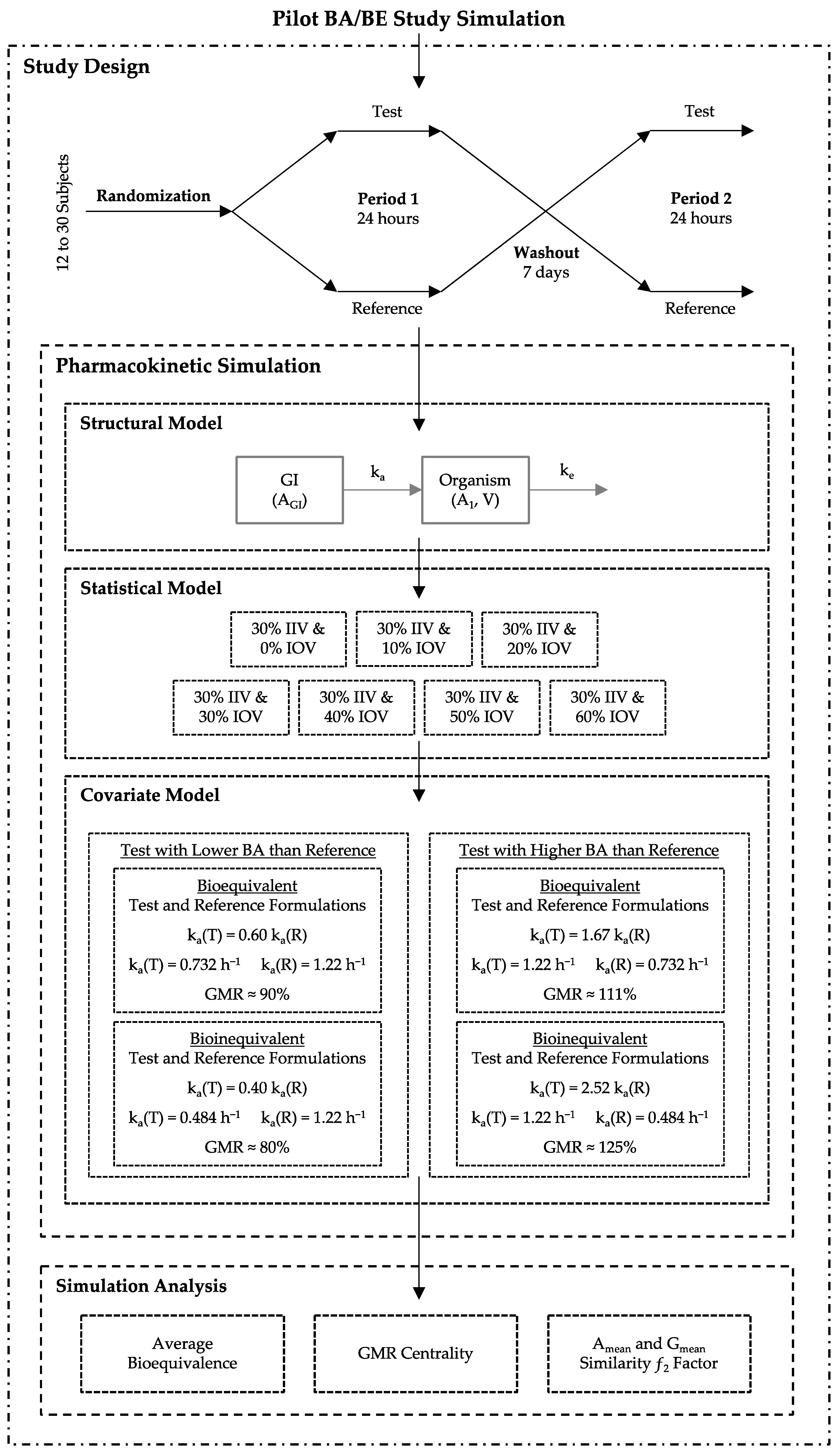
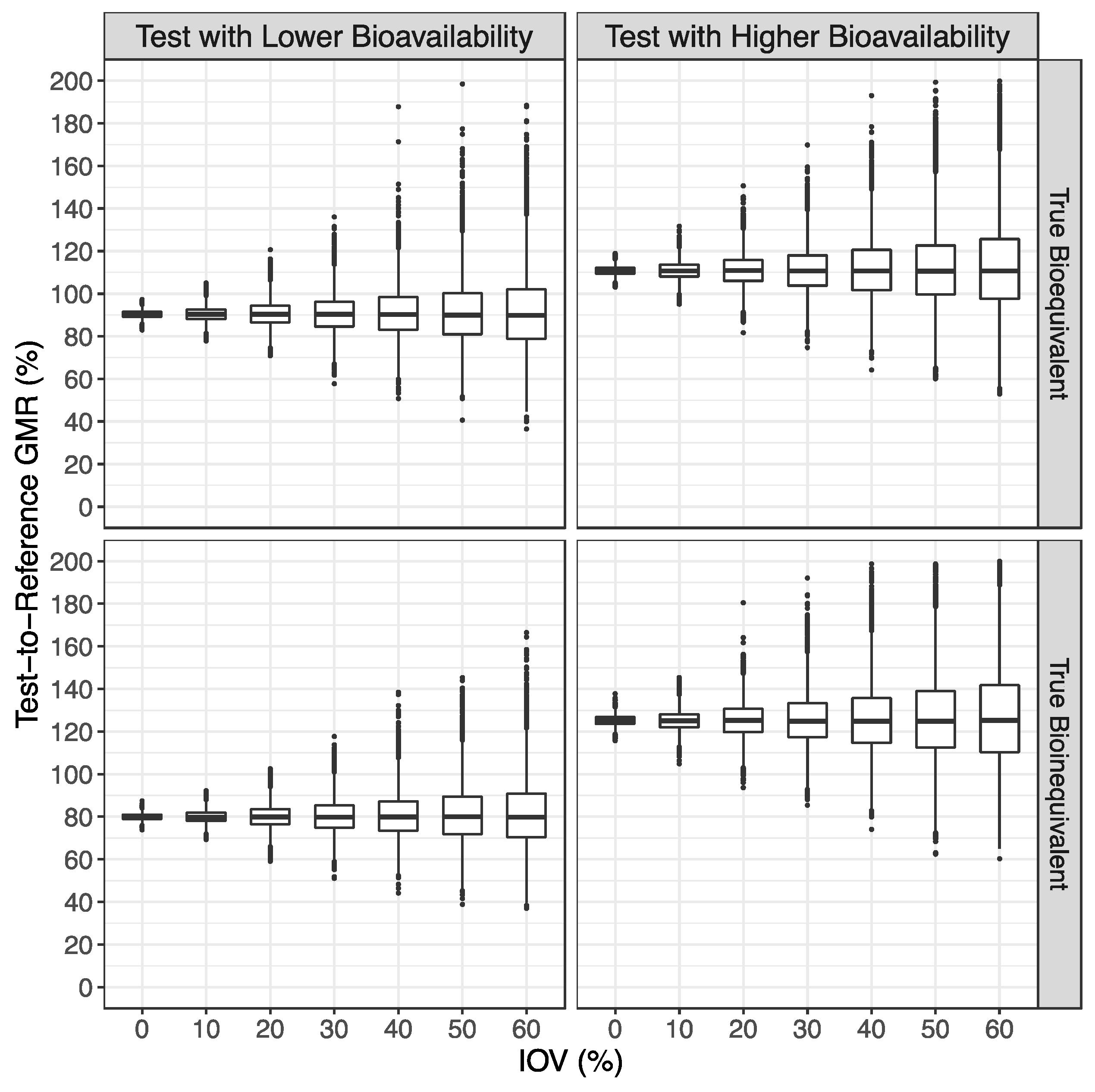
- The Test product presents a lower bioavailability (BA) than the Reference product, with a true GMR of 90% (truly bioequivalent formulations) and 80% (truly bioinequivalent formulations).
- The Test product presents a higher bioavailability than the Reference product, with a true GMR of 111% (truly bioequivalent formulations) and 125% (truly bioinequivalent formulations).
2. Materials and Methods
2.1. Study Design and Pharmacokinetic Simulation
2.2. Simulation Bioequivalence Analysis
3. Results
3.1. Simulated Pharmacokinetic Data
3.2. Bioequivalence Evaluation
4. Discussion
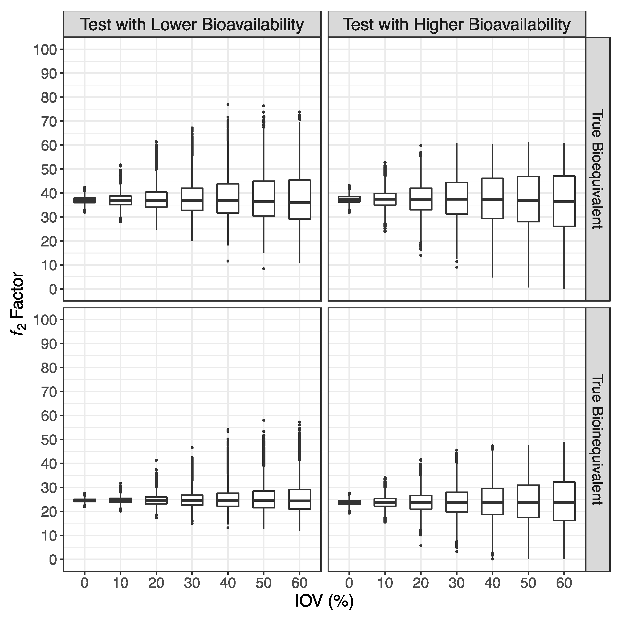
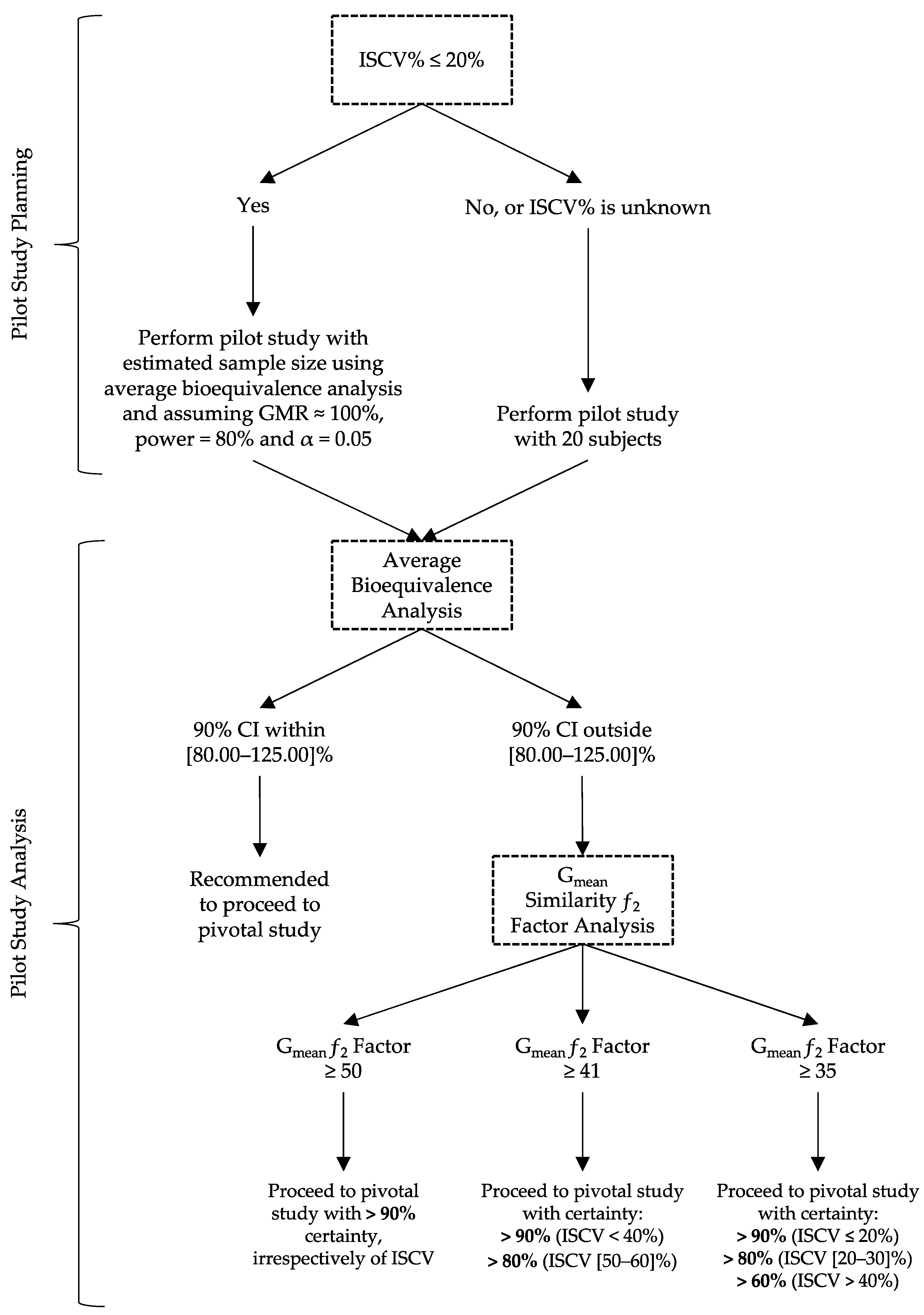
- If the ƒ2 factor is above or equal to 35 (corresponding to a difference of 20% between Test and Reference concentration–time profiles until the Reference tmax), the confidence to proceed to a pivotal study is higher than 90% when ISCV% is lower or equal to 20%; the confidence is higher than 80% when ISCV% is within 20% and 30%; and the confidence is higher than 60% when ISCV% is higher than 40%.
- If the ƒ2 factor is above or equal to 41 (corresponding to a difference of 15% between Test and Reference concentration–time profiles until the Reference tmax), the confidence to proceed to a pivotal study is higher than 90% for ISCV% until 40%, and higher than 80% for ISCV% within 50% to 60%.
- If the ƒ2 factor is above or equal to 50 (corresponding to a difference of 10% between Test and Reference concentration–time profiles until the Reference tmax), the probability of the Test product to be truly bioequivalent to the Reference product in terms of Cmax, i.e., the confidence to proceed to a pivotal study, is higher than 90%, irrespective of the ISCV%.
5. Conclusions
Supplementary Materials
Author Contributions
Funding
Institutional Review Board Statement
Informed Consent Statement
Data Availability Statement
Conflicts of Interest
References
- European Medicines Agency (EMA). Guideline on the Investigation of Bioequivalence (CPMP/EWP/QWP/1401/98 Rev. 1/ Corr **). London. 20 January 2010. Available online: https://www.ema.europa.eu/en/documents/scientific-guideline/guideline-investigation-bioequivalence-rev1_en.pdf (accessed on 29 August 2023).
- U.S. Food and Drug Administration (FDA). Guidance for Industry: Bioequivalence Studies with Pharmacokinetic Endpoints for Drugs Submitted under an ANDA. Draft Guidance. August 2021. Available online: https://www.fda.gov/media/87219/download (accessed on 29 August 2023).
- Henriques, S.C.; Albuquerque, J.; Paixão, P.; Almeida, L.; Silva, N.E. Alternative Analysis Approaches for the Assessment of Pilot Bioavailability / Bioequivalence Studies. Pharmaceutics 2023, 15, 1430. [Google Scholar] [CrossRef] [PubMed]
- Fuglsang, A. Pilot and Repeat Trials as Development Tools Associated with Demonstration of Bioequivalence. AAPS J. 2015, 17, 678–683. [Google Scholar] [CrossRef]
- Pan, G.; Wang, Y. Average Bioequivalence Evaluation: General Methods for Pilot Trials. J. Biopharm. Stat. 2006, 16, 207–225. [Google Scholar] [CrossRef] [PubMed]
- Moreno, I.; Ochoa, D.; Román, M.; Cabaleiro, T.; Abad-Santos, F. Utility of Pilot Studies for Predicting Ratios and Intrasubject Variability in High-Variability Drugs. Basic Clin. Pharmacol. Toxicol. 2016, 119, 215–221. [Google Scholar] [CrossRef]
- Bonate, P.L. Pharmacokinetic-Pharmacodynamic Modeling and Simulation, 2nd ed.; Springer: New York, NY, USA, 2011; ISBN 978-1-4419-9485-1. [Google Scholar]
- European Medicines Agency (EMA). Questions & Answers: Positions on Specific Questions Addressed to the Pharmacokinetics Working Party (PKWP) (EMA/618604/2008 Rev. 13). 19 November 2015. Available online: https://www.ema.europa.eu/en/documents/scientific-guideline/questions-answers-positions-specific-questions-addressed-pharmacokinetics-working-party_en.pdf (accessed on 29 August 2023).
- European Medicines Agency (EMA). Guideline on the Investigation of Bioequivalence—Annex I. 21 September 2016. Available online: https://www.ema.europa.eu/en/documents/other/31-annex-i-statistical-analysis-methods-compatible-ema-bioequivalence-guideline_en.pdf (accessed on 29 August 2023).
- U.S. Food and Drug Administration (FDA). Guidance for Industry: Statistical Approaches to Establishing Bioequivalence. Draft Guidance. December 2022. Available online: https://www.fda.gov/media/163638/download (accessed on 29 August 2023).
- Schuirmann, D.J. A Comparison of the Two One-Sided Tests Procedure and the Power. J. Pharmacokinet. Biopharm. 1987, 15, 657–680. [Google Scholar] [CrossRef]
- Chow, S.C.; Liu, J. Design and Analysis of Bioavailability and Bioequivalence Studies; Chapman and Hall/CRC: New York, NY, USA, 2008; ISBN 9780429140365. [Google Scholar]
- Chow, S.C. Bioavailability and Bioequivalence in Drug Development. Wiley Interdiscip. Rev. Comput. Stat. 2014, 6, 304–312. [Google Scholar] [CrossRef] [PubMed]
- Moore, J.W.; Flanner, H.H. Mathematical Comparison of Curves with an Emphasis on in Vitro Dissolution Profiles. Pharm. Technol. 1996, 20, 64–74. [Google Scholar]
- Kuhn, M. Building Predictive Models in R Using the Caret Package. J. Stat. Softw. 2008, 28, 1–26. [Google Scholar] [CrossRef]
- Chicco, D.; Tötsch, N.; Jurman, G. The Matthews Correlation Coefficient (MCC) Is More Reliable than Balanced Accuracy, Bookmaker Informedness, and Markedness in Two-Class Confusion Matrix Evaluation. BioData Min. 2021, 14, 1–22. [Google Scholar] [CrossRef] [PubMed]


| Average Bioequivalence | GMR Centrality | Amean ƒ2 Factor | Gmean ƒ2 Factor | |
|---|---|---|---|---|
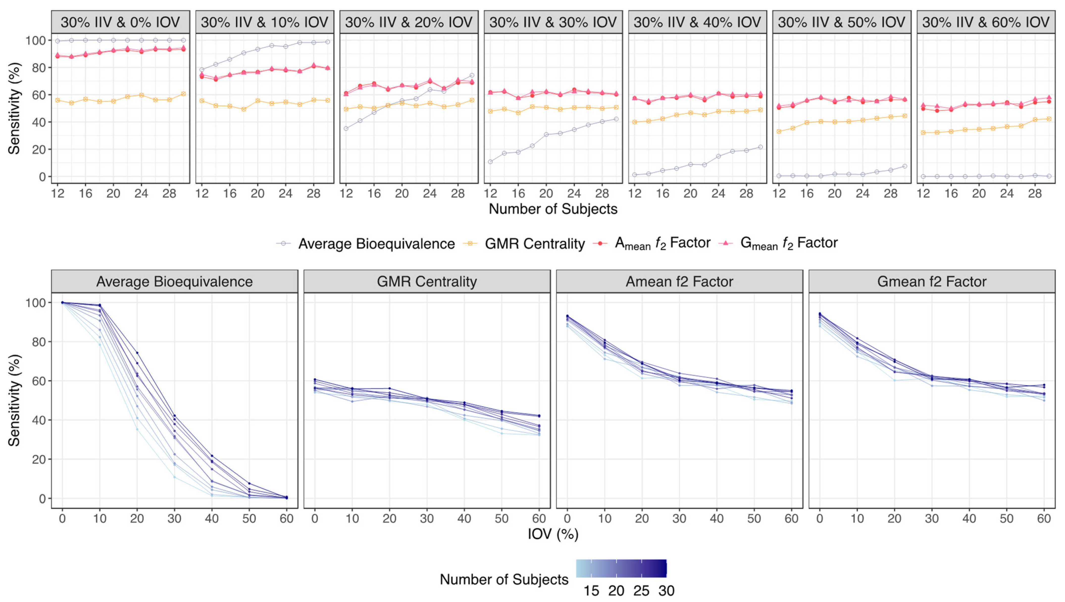
| Sensitivity (%) | ||||
| 30% IIV &0% IOV | 99.4–100 | 56.0–60.7 | 88.1–93.2 | 89.1–94.4 |
| 30% IIV & 10% IOV | 78.4–98.8 | 55.6–55.9 | 73.1–79.5 | 74.9–79.5 |
| 30% IIV &20% IOV | 35.2–74.3 | 49.5–56.1 | 61.3–68.8 | 60.2–69.7 |
| 30% IIV &30% IOV | 10.8–42.2 | 47.9–50.8 | 61.9–60.2 | 61.3–60.8 |
| 30% IIV &40% IOV | 1.30–21.7 | 40.0–48.9 | 57.6–58.8 | 57.2–60.7 |
| 30% IIV &50% IOV | 0.50–7.60 | 33.1–44.5 | 50.4–56.4 | 51.8–56.6 |
| 30% IIV &60% IOV | 0.00–0.30 | 32.2–42.3 | 49.7–55.0 | 52.3–57.9 |
| Type II Error (%) | ||||
| 30% IIV &0% IOV | 0.60–0.00 | 44.0–39.3 | 11.9–6.80 | 10.9–5.60 |
| 30% IIV &10% IOV | 21.6–1.20 | 44.4–44.1 | 26.9–20.5 | 25.1–20.5 |
| 30% IIV &20% IOV | 64.8–25.7 | 50.5–43.9 | 38.7–31.2 | 39.8–30.3 |
| 30% IIV &30% IOV | 89.2–57.8 | 52.1–49.2 | 38.1–39.8 | 38.7–39.2 |
| 30% IIV &40% IOV | 98.7–78.3 | 60.0–51.1 | 42.4–41.2 | 42.8–39.3 |
| 30% IIV &50% IOV | 100–92.4 | 66.9–55.5 | 49.6–43.6 | 48.2–43.4 |
| 30% IIV &60% IOV | 100–99.7 | 67.8–57.7 | 50.3–45.0 | 47.7–42.1 |
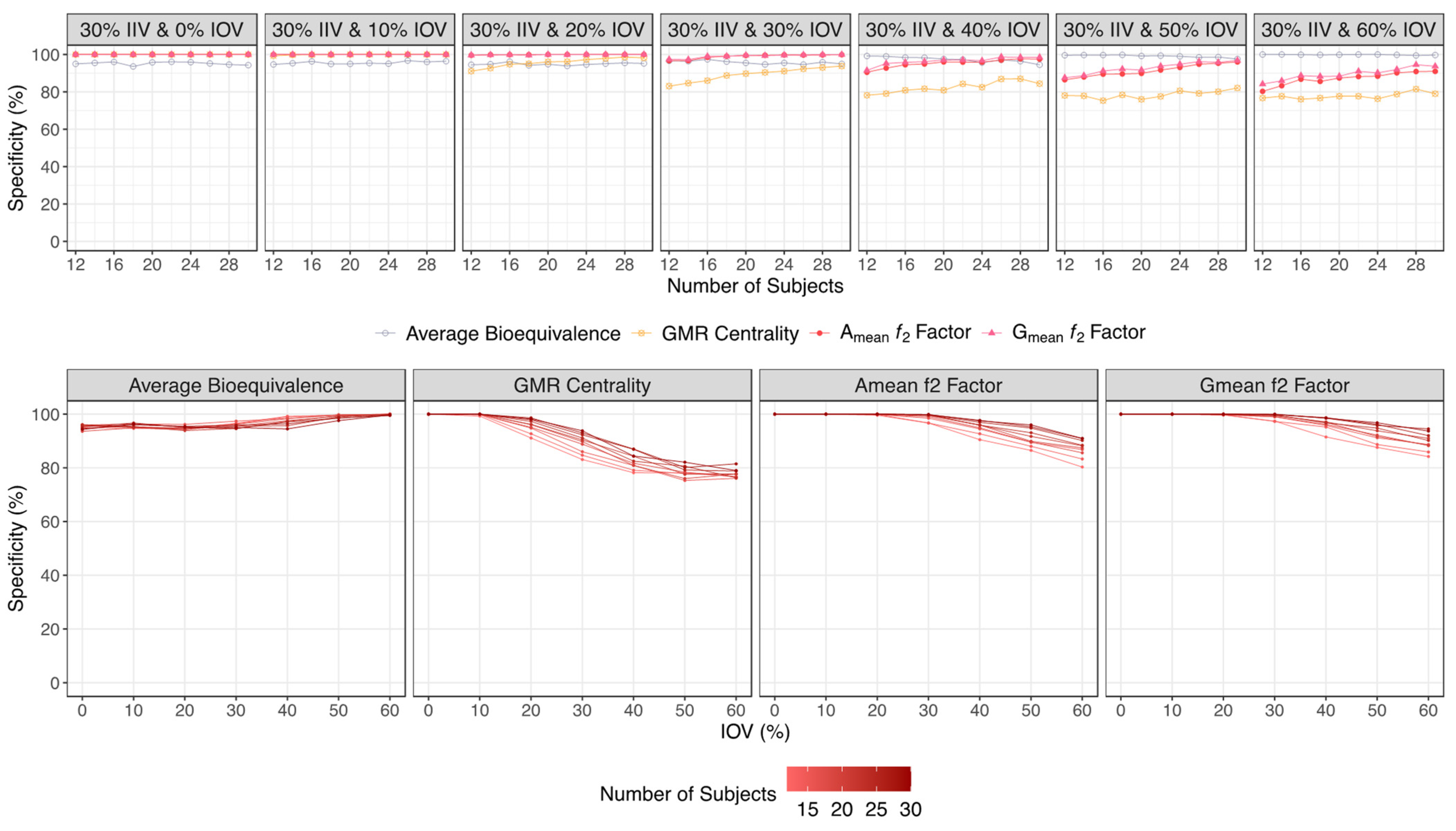
| Specificity (%) | ||||
| 30% IIV & 0% IOV | 95.0–94.3 | 100 | 100 | 100 |
| 30% IIV & 10% IOV | 94.7–96.4 | 99.3–100 | 100 | 100 |
| 30% IIV & 20% IOV | 94.5–95.2 | 91.1–98.2 | 99.6–100 | 99.7–100 |
| 30% IIV & 30% IOV | 96.6–95.0 | 83.1–93.8 | 96.7–100 | 97.4–100 |
| 30% IIV & 40% IOV | 99.2–94.5 | 78.2–84.4 | 90.5–97.5 | 91.5–98.5 |
| 30% IIV & 50% IOV | 100–97.6 | 78.1–82.1 | 86.5–96.0 | 87.6–96.8 |
| 30% IIV & 60% IOV | 100–99.7 | 76.7–79.0 | 80.3–91.0 | 84.2–93.7 |
| Type I Error (%) | ||||
| 30% IIV & 0% IOV | 5.00–5.70 | 0.00 | 0.00 | 0.00 |
| 30% IIV & 10% IOV | 5.30–3.60 | 0.70–0.00 | 0.00 | 0.00 |
| 30% IIV & 20% IOV | 5.50–4.80 | 8.90–1.80 | 0.40–0.00 | 0.30–0.00 |
| 30% IIV & 30% IOV | 3.40–5.00 | 16.9–6.20 | 3.30–0.10 | 2.60–0.00 |
| 30% IIV & 40% IOV | 0.80–5.50 | 21.8–15.6 | 9.5–2.50 | 8.50–1.50 |
| 30% IIV & 50% IOV | 0.40–2.40 | 21.9–17.9 | 13.5–4.00 | 12.4–3.20 |
| 30% IIV & 60% IOV | 0.00–0.30 | 23.3–21.0 | 19.7–9.00 | 15.8–5.50 |
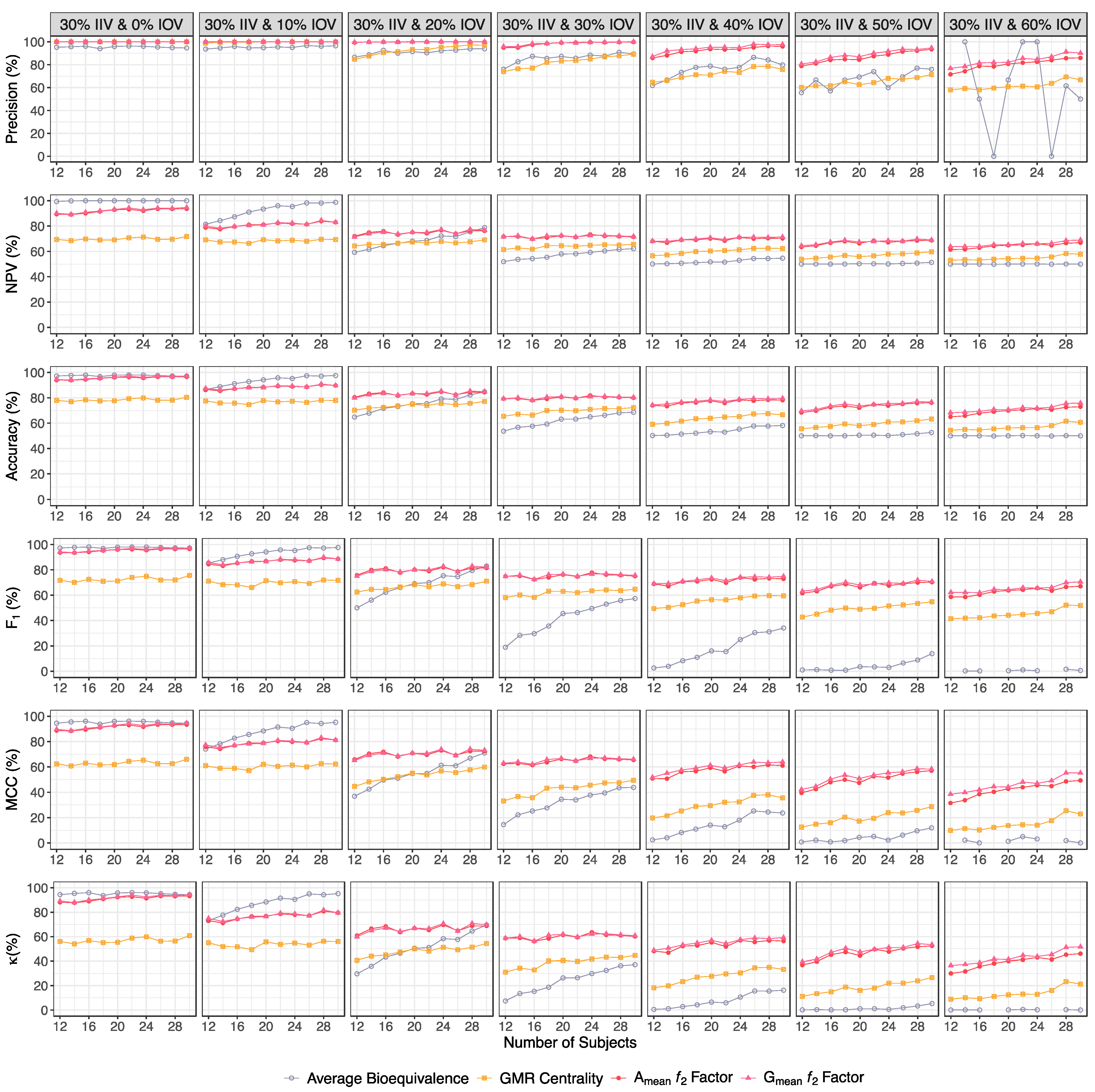
| Precision (%) | ||||
| 30% IIV & 0% IOV | 95.2–94.6 | 100 | 100 | 100 |
| 30% IIV & 10% IOV | 93.7–96.5 | 98.8–100 | 100 | 100 |
| 30% IIV & 20% IOV | 86.5–93.9 | 84.8–96.9 | 99.4–100 | 100–100 |
| 30% IIV & 30% IOV | 76.1–89.4 | 73.9–89.1 | 94.9–100 | 95.9–100 |
| 30% IIV & 40% IOV | 61.9–79.8 | 64.7–75.8 | 85.8–95.9 | 87.1–97.6 |
| 30% IIV & 50% IOV | 55.6–76.0 | 60.2–71.3 | 78.9–93.4 | 80.7–94.6 |
| 30% IIV & 60% IOV | NC–50.0 | 58.0–66.8 | 71.6–85.9 | 76.8–90.2 |
| NPV (%) | ||||
| 30% IIV & 0% IOV | 99.4–100 | 69.4–71.8 | 89.4–93.6 | 90.2–94.7 |
| 30% IIV & 10% IOV | 81.4–98.8 | 69.1–69.4 | 78.8–83.0 | 79.9–83.0 |
| 30% IIV & 20% IOV | 59.3–78.7 | 64.3–69.1 | 72.0–76.2 | 71.5–76.7 |
| 30% IIV & 30% IOV | 52.0–62.2 | 61.5–65.6 | 71.7–71.5 | 71.6–71.8 |
| 30% IIV & 40% IOV | 50.1–54.7 | 56.6–62.3 | 68.1–70.3 | 68.1–71.5 |
| 30% IIV & 50% IOV | 50.0–51.4 | 53.9–59.7 | 63.6–68.8 | 64.5–69.0 |
| 30% IIV & 60% IOV | 50.0 | 53.1–57.8 | 61.5–66.9 | 63.8–69.0 |
| Accuracy (%) | ||||
| 30% IIV & 0% IOV | 97.2–97.2 | 78.0–80.4 | 94.1–96.6 | 94.6–97.2 |
| 30% IIV & 10% IOV | 86.6–97.6 | 77.5–78.0 | 86.6–89.8 | 87.5–89.8 |
| 30% IIV & 20% IOV | 64.9–84.8 | 70.3–77.2 | 80.5–84.4 | 80.0–84.9 |
| 30% IIV & 30% IOV | 53.7–68.6 | 65.5–72.3 | 79.3–80.1 | 79.4–80.4 |
| 30% IIV & 40% IOV | 50.3–58.1 | 59.1–66.7 | 74.1–78.2 | 74.4–79.6 |
| 30% IIV & 50% IOV | 50.1–52.6 | 55.6–63.3 | 68.5–76.2 | 69.7–76.7 |
| 30% IIV & 60% IOV | 50.0 | 54.5–60.7 | 65.0–73.0 | 68.3–75.8 |
| F1 (%) | ||||
| 30% IIV & 0% IOV | 97.3–97.2 | 71.8–75.5 | 93.7–96.5 | 94.2–97.1 |
| 30% IIV & 10% IOV | 85.4–97.6 | 71.1–71.7 | 84.5–88.6 | 85.6–88.6 |
| 30% IIV & 20% IOV | 50.0–83.0 | 62.5–71.1 | 75.8–81.5 | 75.0–82.1 |
| 30% IIV & 30% IOV | 18.9–57.3 | 58.1–64.7 | 74.9–75.1 | 74.8–75.6 |
| 30% IIV & 40% IOV | 2.55–34.1 | 49.4–59.5 | 68.9–72.9 | 69.0–74.8 |
| 30% IIV & 50% IOV | 0.99–13.8 | 42.7–54.8 | 61.5–70.3 | 63.1–70.8 |
| 30% IIV & 60% IOV | NC–0.60 | 41.4–51.8 | 58.7–67.1 | 62.2–70.5 |
| MCC (%) | ||||
| 30% IIV & 0% IOV | 94.5–94.5 | 62.4–66.0 | 88.7–93.4 | 89.6–94.5 |
| 30% IIV & 10% IOV | 74.1–95.2 | 61.0–62.3 | 75.9–81.2 | 77.4–81.2 |
| 30% IIV & 20% IOV | 36.9–71.1 | 44.6–59.9 | 65.9–72.4 | 65.2–73.1 |
| 30% IIV & 30% IOV | 14.4–43.8 | 33.1–49.4 | 62.5–65.5 | 62.9–66.1 |
| 30% IIV & 40% IOV | 2.45–23.6 | 19.7–35.6 | 50.9–61.1 | 51.8–63.9 |
| 30% IIV & 50% IOV | 0.75–11.9 | 12.5–28.7 | 39.6–57.1 | 42.2–58.3 |
| 30% IIV & 60% IOV | NC–0.00 | 9.9–22.9 | 31.5–49.3 | 38.5–55.3 |
| κ (%) | ||||
| 30% IIV & 0% IOV | 94.4–94.3 | 56.0–60.7 | 88.1–93.2 | 89.1–94.4 |
| 30% IIV & 10% IOV | 73.1–95.2 | 54.9–55.9 | 73.1–79.5 | 74.9–79.5 |
| 30% IIV & 20% IOV | 29.7–69.5 | 40.6–54.3 | 60.9–68.8 | 59.9–69.7 |
| 30% IIV & 30% IOV | 7.40–37.2 | 31.0–44.6 | 58.6–60.1 | 58.7–60.8 |
| 30% IIV & 40% IOV | 0.50–16.2 | 18.2–33.3 | 48.1–56.3 | 48.7–59.2 |
| 30% IIV & 50% IOV | 0.10–5.20 | 11.2–26.6 | 36.9–52.4 | 39.4–53.4 |
| 30% IIV & 60% IOV | 0.00 | 8.90–21.3 | 30.0–46.0 | 36.5–51.6 |
| Average Bioequivalence | GMR Centrality | Amean ƒ2 Factor | Gmean ƒ2 Factor | |
|---|---|---|---|---|
| Sensitivity (%) | ||||
| 30% IIV & 0% IOV | 100 | 53.4–60.5 | 87.2–95.6 | 89.5–97.0 |
| 30% IIV & 10% IOV | 77.7–99.0 | 54.1–51.6 | 70.5–75.3 | 71.4–77.6 |
| 30% IIV & 20% IOV | 36.2–67.6 | 51.7–49.9 | 63.5–62.5 | 62.8–62.5 |
| 30% IIV & 30% IOV | 11.1–43.7 | 46.3–53.4 | 57.4–61.3 | 58.0–61.6 |
| 30% IIV & 40% IOV | 2.30–19.8 | 42.4–48.3 | 55.4–58.1 | 57.3–58.6 |
| 30% IIV & 50% IOV | 0.30–7.00 | 34.8–45.1 | 50.0–56.2 | 52.6–56.1 |
| 30% IIV & 60% IOV | 0.00–1.30 | 29.7–44.3 | 46.9–52.9 | 48.2–56.5 |
| Type II Error (%) | ||||
| 30% IIV & 0% IOV | 0.00 | 46.6–39.5 | 12.8–4.40 | 10.5–3.00 |
| 30% IIV & 10% IOV | 22.3–1.00 | 45.9–48.4 | 29.5–24.7 | 28.6–22.4 |
| 30% IIV & 20% IOV | 63.8–32.4 | 48.3–50.1 | 36.5–37.5 | 37.2–37.5 |
| 30% IIV & 30% IOV | 88.9–56.3 | 53.7–46.6 | 42.6–38.7 | 42.0–38.4 |
| 30% IIV & 40% IOV | 97.7–80.2 | 57.6–51.7 | 44.6–41.9 | 42.7–41.4 |
| 30% IIV & 50% IOV | 100–93.0 | 65.2–54.9 | 50.0–43.8 | 47.4–43.9 |
| 30% IIV & 60% IOV | 100–98.7 | 70.3–55.7 | 53.1–47.1 | 51.8–43.5 |
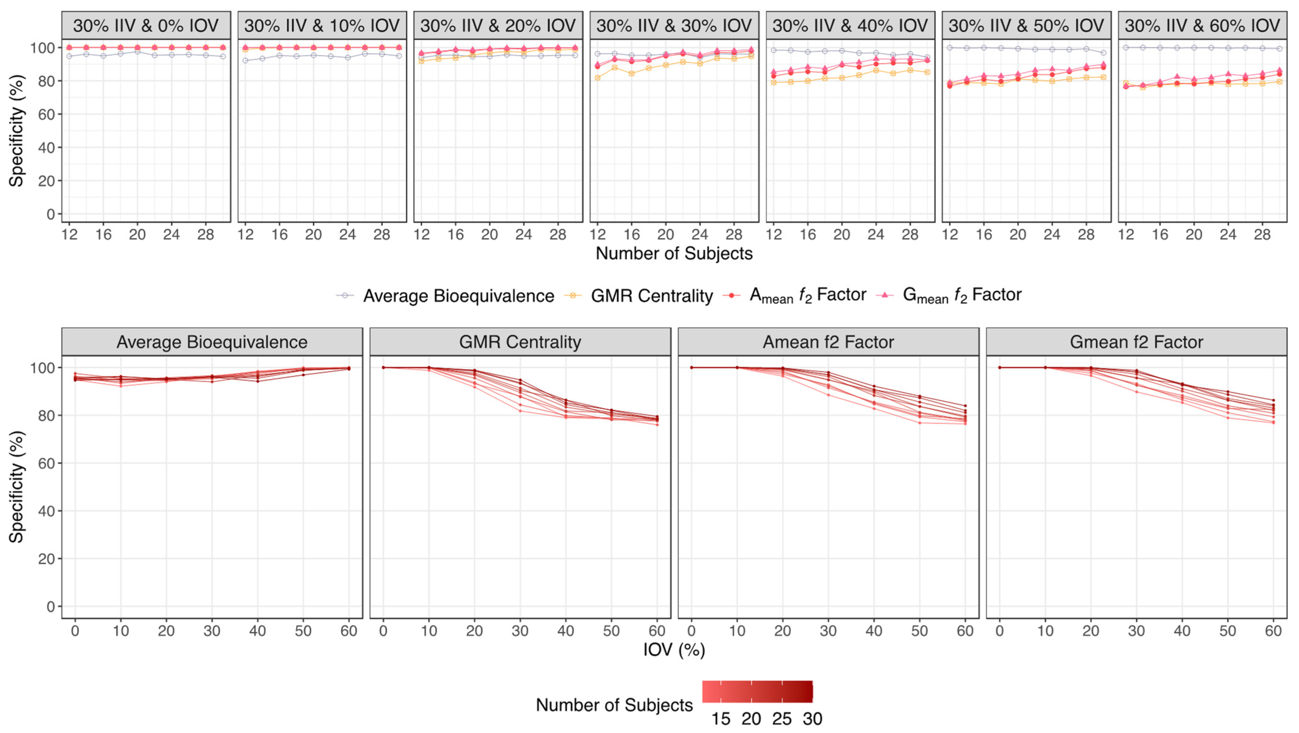
| Specificity (%) | ||||
| 30% IIV & 0% IOV | 94.8–94.7 | 100 | 100 | 100 |
| 30% IIV & 10% IOV | 92.2–95.0 | 98.8–100 | 100–100 | 100 |
| 30% IIV & 20% IOV | 94.0–95.3 | 91.8–98.9 | 96.4–100 | 96.6–100 |
| 30% IIV & 30% IOV | 96.3–96.0 | 81.8–94.8 | 88.5–98.0 | 89.8–98.8 |
| 30% IIV & 40% IOV | 98.4–94.2 | 79.0–85.2 | 82.8–92.2 | 85.3–92.6 |
| 30% IIV & 50% IOV | 100–96.9 | 78.5–82.2 | 76.8–88.0 | 78.9–89.9 |
| 30% IIV & 60% IOV | 100–99.3 | 78.7–79.5 | 76.4–84.0 | 76.8–86.3 |
| Type I Error (%) | ||||
| 30% IIV & 0% IOV | 5.20–5.30 | 0.00 | 0.00 | 0.00 |
| 30% IIV & 10% IOV | 7.80–5.00 | 1.20–0.00 | 0.10–0.00 | 0.00 |
| 30% IIV & 20% IOV | 6.00–4.70 | 8.20–1.10 | 3.60–0.20 | 3.40–0.10 |
| 30% IIV & 30% IOV | 3.70–4.00 | 18.2–5.20 | 11.5–2.00 | 10.2–1.20 |
| 30% IIV & 40% IOV | 1.60–5.80 | 21.0–14.8 | 17.2–7.80 | 14.7–7.40 |
| 30% IIV & 50% IOV | 0.10–3.10 | 21.5–17.8 | 23.2–12.0 | 21.1–10.1 |
| 30% IIV & 60% IOV | 0.00–0.70 | 21.3–20.5 | 23.6–16.0 | 23.2–13.7 |
| Precision (%) | ||||
| 30% IIV & 0% IOV | 95.1–95.0 | 100 | 100 | 100 |
| 30% IIV & 10% IOV | 90.9–95.2 | 97.8–100 | 100 | 100 |
| 30% IIV & 20% IOV | 85.8–93.5 | 86.3–97.8 | 94.6–100 | 94.9–100 |
| 30% IIV & 30% IOV | 75.0–91.6 | 71.8–91.1 | 83.3–96.8 | 85.0–98.1 |
| 30% IIV & 40% IOV | 59.0–77.3 | 66.9–76.5 | 76.3–88.2 | 79.6–88.8 |
| 30% IIV & 50% IOV | 75.0–69.3 | 61.8–71.7 | 68.3–82.4 | 71.4–84.7 |
| 30% IIV & 60% IOV | NC–65.0 | 58.2–68.4 | 66.5–76.8 | 67.5–80.5 |
| NPV (%) | ||||
| 30% IIV & 0% IOV | 100 | 68.2–71.7 | 88.7–95.8 | 90.5–97.1 |
| 30% IIV & 10% IOV | 80.5–99.0 | 68.3–67.4 | 77.2–80.2 | 77.8–81.7 |
| 30% IIV & 20% IOV | 59.6–74.6 | 65.5–66.4 | 72.5–72.7 | 72.2–72.7 |
| 30% IIV & 30% IOV | 52.0–63.0 | 60.4–67.0 | 67.5–71.7 | 68.1–72.0 |
| 30% IIV & 40% IOV | 50.2–54.0 | 57.8–62.2 | 65.0–68.8 | 66.6–69.1 |
| 30% IIV & 50% IOV | 50.1–51.0 | 54.6–60.0 | 60.6–66.8 | 62.5–67.2 |
| 30% IIV & 60% IOV | 50.0–50.2 | 52.8–58.8 | 59.0–64.1 | 59.7–66.5 |
| Accuracy (%) | ||||
| 30% IIV & 0% IOV | 97.4–97.4 | 76.7–80.3 | 93.6–97.8 | 94.8–98.5 |
| 30% IIV & 10% IOV | 85.0–97.0 | 76.5–75.8 | 85.2–87.7 | 85.7–88.8 |
| 30% IIV & 20% IOV | 65.1–81.5 | 71.8–74.4 | 80.0–81.2 | 79.7–81.2 |
| 30% IIV & 30% IOV | 53.7–69.9 | 64.1–74.1 | 73.0–79.7 | 73.9–80.2 |
| 30% IIV & 40% IOV | 50.4–57.0 | 60.7–66.8 | 69.1–75.2 | 71.3–75.6 |
| 30% IIV & 50% IOV | 50.1–52.0 | 56.7–63.7 | 63.4–72.1 | 65.8–73.0 |
| 30% IIV & 60% IOV | 50.0–50.3 | 54.2–61.9 | 61.7–68.5 | 62.5–71.4 |
| F1 (%) | ||||
| 30% IIV & 0% IOV | 97.5–97.4 | 69.6–75.4 | 93.2–97.8 | 94.5–98.5 |
| 30% IIV & 10% IOV | 83.8–97.1 | 69.7–68.1 | 82.6–85.9 | 83.3–87.4 |
| 30% IIV & 20% IOV | 50.9–78.5 | 64.7–66.1 | 76.0–76.8 | 75.6–76.9 |
| 30% IIV & 30% IOV | 19.3–59.2 | 56.3–67.3 | 68.0–75.1 | 69.0–75.7 |
| 30% IIV & 40% IOV | 4.43–31.5 | 51.9–59.2 | 64.2–70.0 | 66.6–70.6 |
| 30% IIV & 50% IOV | 0.60–12.7 | 44.5–55.4 | 57.7–66.8 | 60.6–67.5 |
| 30% IIV & 60% IOV | NC–2.55 | 39.3–53.8 | 55.0–62.6 | 56.2–66.4 |
| MCC (%) | ||||
| 30% IIV & 0% IOV | 94.9–94.8 | 60.4–65.9 | 87.9–95.7 | 90.0–97.0 |
| 30% IIV & 10% IOV | 70.6–94.1 | 59.1–59.0 | 73.7–77.7 | 74.5–79.6 |
| 30% IIV & 20% IOV | 37.0–65.5 | 47.5–56.0 | 63.4–67.1 | 63.1–67.3 |
| 30% IIV & 30% IOV | 14.1–46.6 | 30.1–53.0 | 48.3–63.7 | 50.4–65.1 |
| 30% IIV & 40% IOV | 2.53–21.0 | 23.0–36.0 | 39.7–53.5 | 44.4–54.4 |
| 30% IIV & 50% IOV | 2.24–8.91 | 14.8–29.4 | 27.8–46.6 | 32.6–48.9 |
| 30% IIV & 60% IOV | NC–3.02 | 9.60–25.4 | 24.4–38.8 | 26.1–44.8 |
| κ (%) | ||||
| 30% IIV & 0% IOV | 94.8–94.7 | 53.4–60.5 | 87.2–95.6 | 89.5–97.0 |
| 30% IIV & 10% IOV | 69.9–94.0 | 52.9–51.6 | 70.4–75.3 | 71.4–77.6 |
| 30% IIV & 20% IOV | 30.2–62.9 | 43.5–48.8 | 59.9–62.3 | 59.4–62.4 |
| 30% IIV & 30% IOV | 7.40–39.7 | 28.1–48.2 | 45.9–59.3 | 47.8–60.4 |
| 30% IIV & 40% IOV | 0.70–14.0 | 21.4–33.5 | 38.2–50.3 | 42.6–51.2 |
| 30% IIV & 50% IOV | 0.20–3.90 | 13.3–27.3 | 26.8–44.2 | 31.5–46.0 |
| 30% IIV & 60% IOV | 0.00–0.60 | 8.40–23.8 | 23.3–36.9 | 25.0–42.8 |
Disclaimer/Publisher’s Note: The statements, opinions and data contained in all publications are solely those of the individual author(s) and contributor(s) and not of MDPI and/or the editor(s). MDPI and/or the editor(s) disclaim responsibility for any injury to people or property resulting from any ideas, methods, instructions or products referred to in the content. |
© 2023 by the authors. Licensee MDPI, Basel, Switzerland. This article is an open access article distributed under the terms and conditions of the Creative Commons Attribution (CC BY) license (https://creativecommons.org/licenses/by/4.0/).
Share and Cite
Henriques, S.C.; Paixão, P.; Almeida, L.; Silva, N.E. Predictive Potential of Cmax Bioequivalence in Pilot Bioavailability/Bioequivalence Studies, through the Alternative ƒ2 Similarity Factor Method. Pharmaceutics 2023, 15, 2498. https://doi.org/10.3390/pharmaceutics15102498
Henriques SC, Paixão P, Almeida L, Silva NE. Predictive Potential of Cmax Bioequivalence in Pilot Bioavailability/Bioequivalence Studies, through the Alternative ƒ2 Similarity Factor Method. Pharmaceutics. 2023; 15(10):2498. https://doi.org/10.3390/pharmaceutics15102498
Chicago/Turabian StyleHenriques, Sara Carolina, Paulo Paixão, Luis Almeida, and Nuno Elvas Silva. 2023. "Predictive Potential of Cmax Bioequivalence in Pilot Bioavailability/Bioequivalence Studies, through the Alternative ƒ2 Similarity Factor Method" Pharmaceutics 15, no. 10: 2498. https://doi.org/10.3390/pharmaceutics15102498