Spatially Resolved Effects of Protein Freeze-Thawing in a Small-Scale Model Using Monoclonal Antibodies


Abstract
:
1. Introduction
2. Materials and Methods
2.1. mABs Production and Purification
2.2. Freeze-Thawing
2.3. Analytics
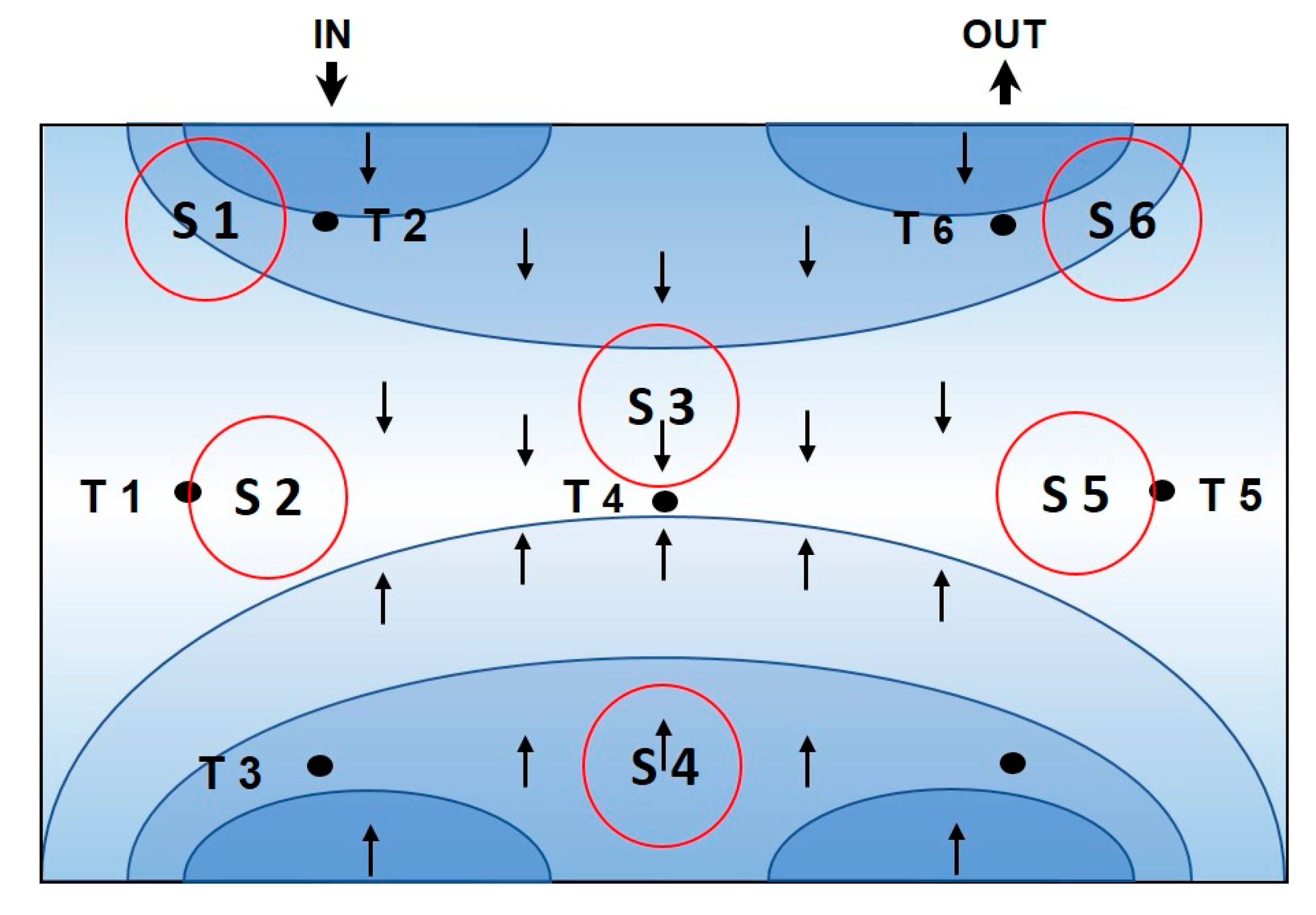
2.3.1. Sampling
2.3.2. Total Protein Concentration
2.3.3. IgG Titer Determination
2.3.4. IgG Aggregate Determination
2.3.5. pH Measurement
2.3.6. Conductivity Measurements
2.3.7. Linear Regression Models
3. Results and Discussion
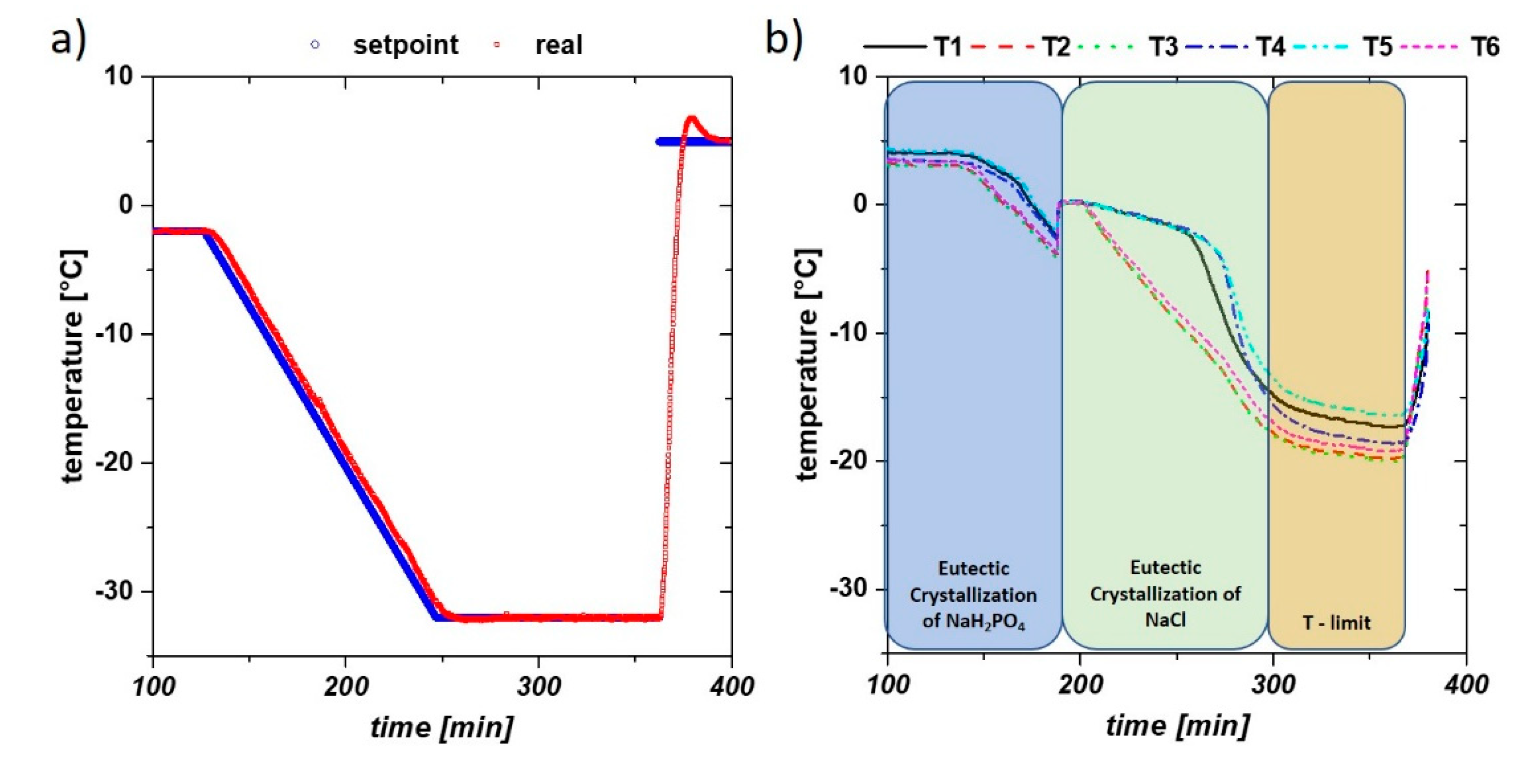
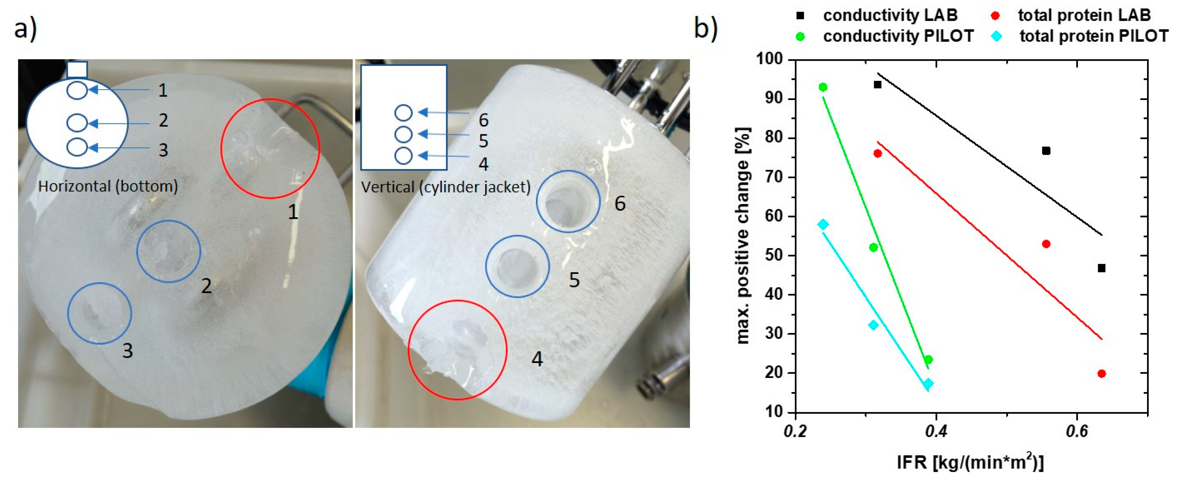
3.1. Rate Experiments and Freezing Characteristics
3.2. pH and Conductivity of the Freezing Formulation
3.3. Effects on Product Quality
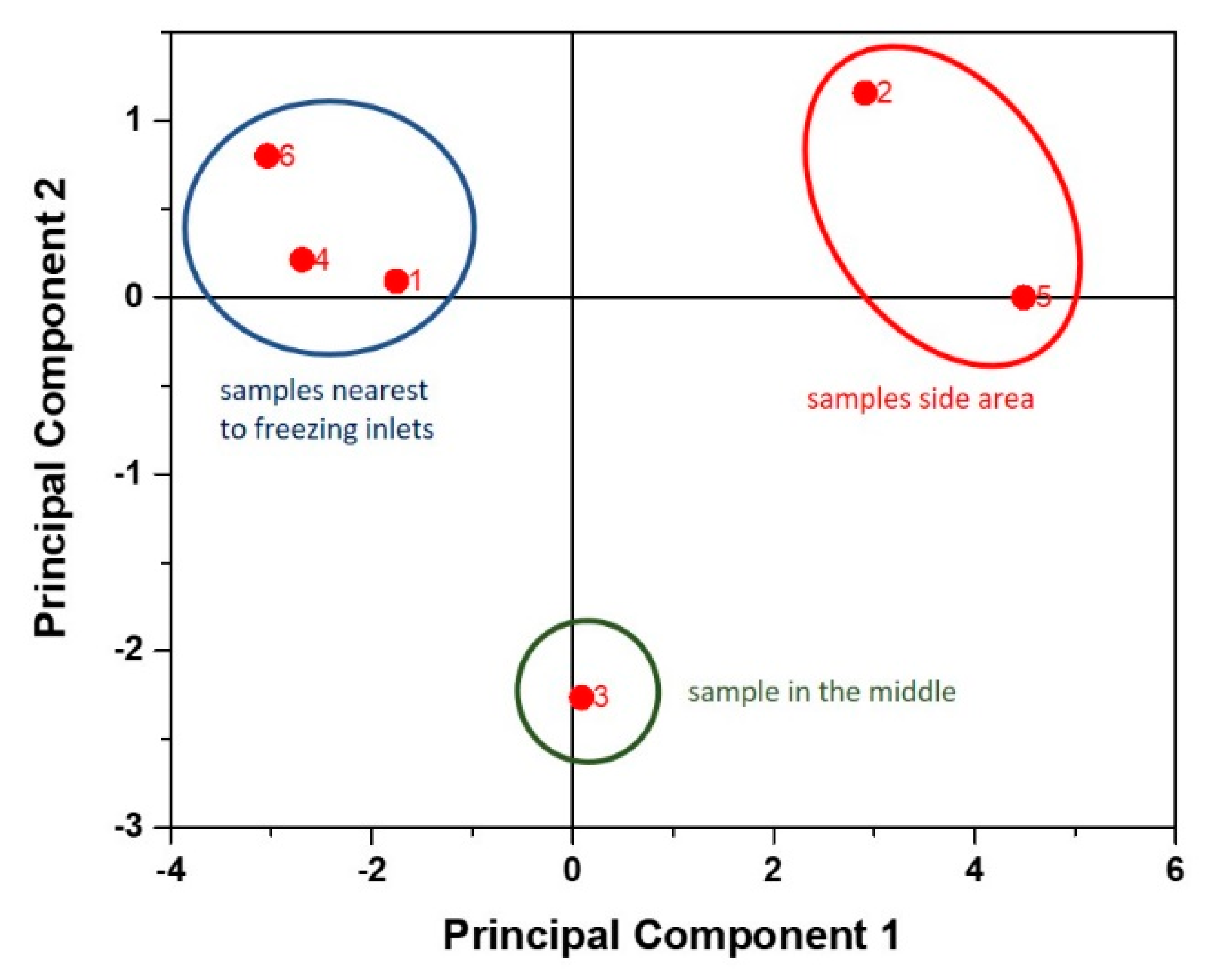
3.4. Multivariate and Mechanistical Description of mAB Freezing
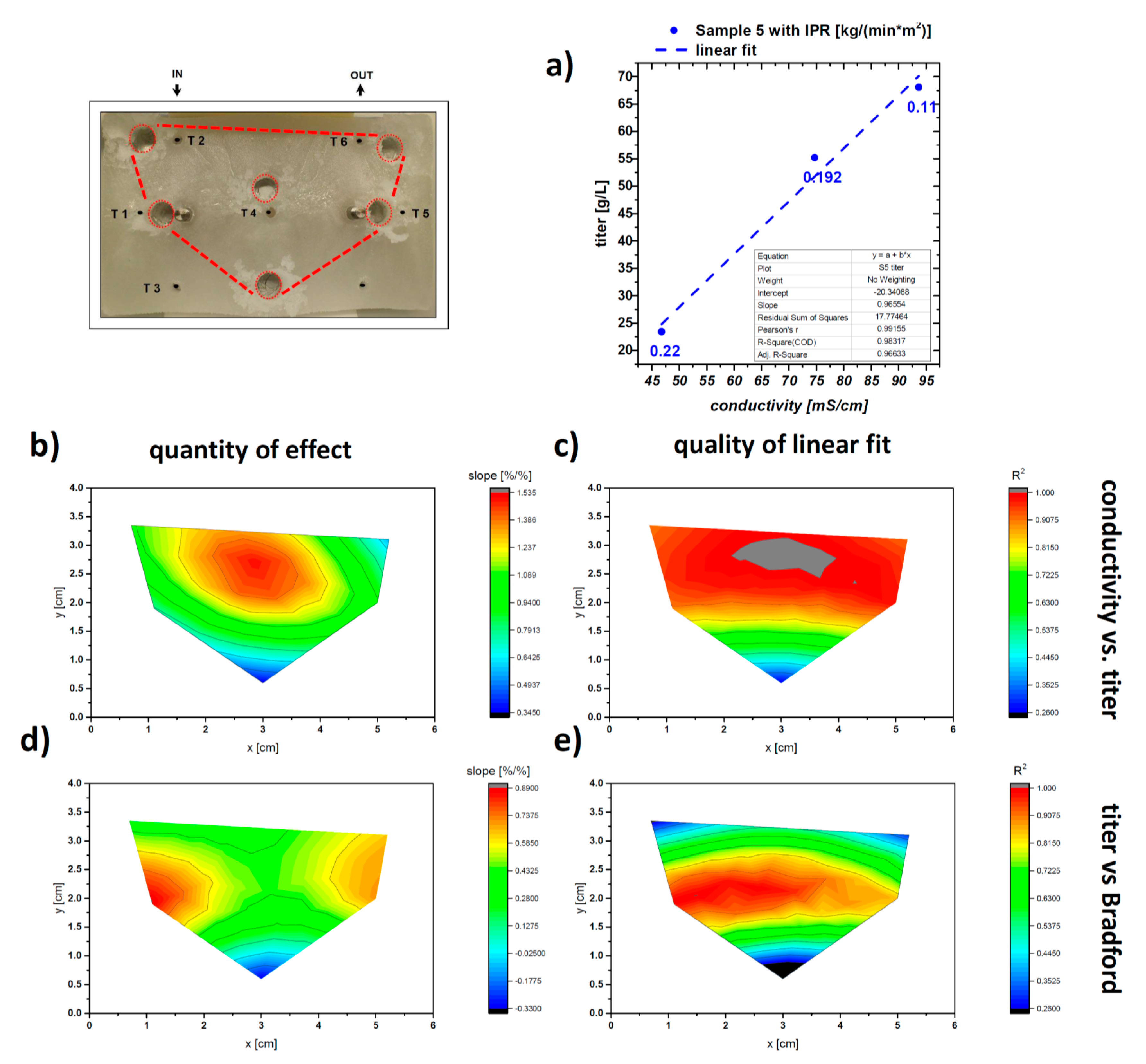
3.5. IFR as Key Parameter for Freeze/Thawing Experiments
4. Conclusions
Supplementary Materials
Author Contributions
Funding
Acknowledgments
Conflicts of Interest
References
- An, Z. Monoclonal antibodies—A proven and rapidly expanding therapeutic modality for human diseases. Protein Cell 2010, 1, 319–330. [Google Scholar] [CrossRef] [PubMed] [Green Version]
- Ecker, D.M.; Jones, S.D.; Levine, H.L. The therapeutic monoclonal antibody market. In MAbs; Taylor & Francis: Milton, UK, 2015; pp. 9–14. [Google Scholar]
- Gronemeyer, P.; Ditz, R.; Strube, J. Trends in upstream and downstream process development for antibody manufacturing. Bioengineering 2014, 1, 188–212. [Google Scholar] [CrossRef] [PubMed] [Green Version]
- Bareither, R.; Pollard, D. A review of advanced small-scale parallel bioreactor technology for accelerated process development: Current state and future need. Biotechnol. Prog. 2011, 27, 2–14. [Google Scholar] [CrossRef] [PubMed]
- Shukla, A.A.; Wolfe, L.S.; Mostafa, S.S.; Norman, C. Evolving trends in mAb production processes. Bioeng. Transl. Med. 2017, 2, 58–69. [Google Scholar] [CrossRef] [PubMed]
- Bielser, J.-M.; Wolf, M.; Souquet, J.; Broly, H.; Morbidelli, M. Perfusion mammalian cell culture for recombinant protein manufacturing–A critical review. Biotechnol. Adv. 2018, 36, 1328–1340. [Google Scholar] [CrossRef] [PubMed]
- Zydney, A.L. Continuous downstream processing for high value biological products: A review. Biotechnol. Bioeng. 2016, 113, 465–475. [Google Scholar] [CrossRef]
- Kolhe, P.; Amend, E.K.; Singh, S. Impact of freezing on pH of buffered solutions and consequences for monoclonal antibody aggregation. Biotechnol. Prog. 2010, 26, 727–733. [Google Scholar] [CrossRef]
- Desai, K.G.; Pruett, W.A.; Martin, P.J.; Colandene, J.D.; Nesta, D.P. Impact of manufacturing-scale freeze-thaw conditions on a mAb solution. BioPharm Int. 2017, 30, 30–36. [Google Scholar]
- Badkar, A.; Wolf, A.; Bohack, L.; Kolhe, P. Development of biotechnology products in pre-filled syringes: Technical considerations and approaches. AAPS PharmSciTech 2011, 12, 564–572. [Google Scholar] [CrossRef] [Green Version]
- Puri, M.; Morar-Mitrica, S.; Crotts, G.; Nesta, D. Evaluating Freeze–Thaw Processes in Biopharmaceutical Development. BioProcess Int. 2015, 13, 34–45. [Google Scholar]
- Arosio, P.; Barolo, G.; Müller-Späth, T.; Wu, H.; Morbidelli, M. Aggregation Stability of a Monoclonal Antibody During Downstream Processing. Pharm. Res. 2011, 28, 1884–1894. [Google Scholar] [CrossRef] [PubMed] [Green Version]
- Stefani, M.; Dobson, C.M. Protein aggregation and aggregate toxicity: New insights into protein folding, misfolding diseases and biological evolution. J. Mol. Med. 2003, 81, 678–699. [Google Scholar] [CrossRef] [PubMed]
- Mahler, H.-C.; Friess, W.; Grauschopf, U.; Kiese, S. Protein aggregation: Pathways, induction factors and analysis. J. Pharm. Sci. 2009, 98, 2909–2934. [Google Scholar] [CrossRef] [PubMed]
- Gerhardt, A.; Mcumber, A.C.; Nguyen, B.H.; Lewus, R.; Schwartz, D.K.; Carpenter, J.F.; Randolph, T.W. Surfactant effects on particle generation in antibody formulations in pre-filled syringes. J. Pharm. Sci. 2015, 104, 4056–4064. [Google Scholar] [CrossRef] [Green Version]
- Dias, C.L.; Ala-Nissila, T.; Karttunen, M.; Vattulainen, I.; Grant, M. Microscopic mechanism for cold denaturation. Phys. Rev. Lett. 2008, 100, 118101. [Google Scholar] [CrossRef] [Green Version]
- Marqués, M.I.; Borreguero, J.M.; Stanley, H.E.; Dokholyan, N.V. Possible Mechanism for Cold Denaturation of Proteins at High Pressure. Phys. Rev. Lett. 2003, 91, 138103. [Google Scholar] [CrossRef] [Green Version]
- Ben-Naim, A. Theory of cold denaturation of proteins. Adv. Biol. Chem. 2013, 3, 29. [Google Scholar] [CrossRef] [Green Version]
- Wang, Y.; Lomakin, A.; Latypov, R.F.; Benedek, G.B. Phase separation in solutions of monoclonal antibodies and the effect of human serum albumin. Proc. Natl. Acad. Sci. USA 2011, 108, 16606–16611. [Google Scholar] [CrossRef] [Green Version]
- Pikal-Cleland, K.A.; Rodríguez-Hornedo, N.; Amidon, G.L.; Carpenter, J.F. Protein denaturation during freezing and thawing in phosphate buffer systems: Monomeric and tetrameric β-galactosidase. Arch. Biochem. Biophys. 2000, 384, 398–406. [Google Scholar] [CrossRef]
- Hauptmann, A.; Hoelzl, G.; Loerting, T. Distribution of Protein Content and Number of Aggregates in Monoclonal Antibody Formulation after Large-Scale Freezing. AAPS PharmSciTech 2019, 20, 72. [Google Scholar] [CrossRef] [Green Version]
- Hawe, A.; Kasper, J.C.; Friess, W.; Jiskoot, W. Structural properties of monoclonal antibody aggregates induced by freeze–thawing and thermal stress. Eur. J. Pharm. Sci. 2009, 38, 79–87. [Google Scholar] [CrossRef] [PubMed]
- Kueltzo, L.A.; Wang, W.; Randolph, T.W.; Carpenter, J.F. Effects of solution conditions, processing parameters, and container materials on aggregation of a monoclonal antibody during freeze–thawing. J. Pharm. Sci. 2008, 97, 1801–1812. [Google Scholar] [CrossRef] [PubMed]
- Reinsch, H.; Spadiut, O.; Heidingsfelder, J.; Herwig, C. Examining the freezing process of an intermediate bulk containing an industrially relevant protein. Enzym. Microb. Technol. 2015, 71, 13–19. [Google Scholar] [CrossRef] [PubMed] [Green Version]
- Wöll, A.K.; Schütz, J.; Zabel, J.; Hubbuch, J. Analysis of phase behavior and morphology during freeze-thaw applications of lysozyme. Int. J. Pharm. 2019, 555, 153–164. [Google Scholar] [CrossRef] [PubMed]
- Brunner, M.; Braun, P.; Doppler, P.; Posch, C.; Behrens, D.; Herwig, C.; Fricke, J. The impact of pH inhomogeneities on CHO cell physiology and fed-batch process performance–two-compartment scale-down modelling and intracellular pH excursion. Biotechnol. J. 2017, 12, 1600633. [Google Scholar] [CrossRef]
- Brunner, M.; Doppler, P.; Klein, T.; Herwig, C.; Fricke, J. Elevated pCO2 affects the lactate metabolic shift in CHO cell culture processes. Eng. Life Sci. 2018, 18, 204–214. [Google Scholar] [CrossRef] [Green Version]
- Daugherty, A.L.; Mrsny, R.J. Formulation and delivery issues for monoclonal antibody therapeutics. Adv. Drug Deliv. Rev. 2006, 58, 686–706. [Google Scholar] [CrossRef]
- Sevanto, S.; Holbrook, N.M.; Ball, M. Freeze/Thaw-Induced Embolism: Probability of Critical Bubble Formation Depends on Speed of Ice Formation. Front. Plant Sci. 2012, 3. [Google Scholar] [CrossRef] [Green Version]
- Arosio, P.; Jaquet, B.; Wu, H.; Morbidelli, M. On the role of salt type and concentration on the stability behavior of a monoclonal antibody solution. Biophys. Chem. 2012, 168, 19–27. [Google Scholar] [CrossRef]
- Schwegman, J.J.; Carpenter, J.F.; Nail, S.L. Evidence of partial unfolding of proteins at the ice/freeze-concentrate interface by infrared microscopy. J. Pharm. Sci. 2009, 98, 3239–3246. [Google Scholar] [CrossRef]
- Krielgaard, L.; Jones, L.S.; Randolph, T.W.; Frokjaer, S.; Flink, J.M.; Manning, M.C.; Carpenter, J.F. Effect of Tween 20 on freeze-thawing-and agitation-induced aggregation of recombinant human factor XIII. J. Pharm. Sci. 1998, 87, 1593–1603. [Google Scholar] [CrossRef] [PubMed]
- Wang, W.; Nema, S.; Teagarden, D. Protein aggregation—pathways and influencing factors. Int. J. Pharm. 2010, 390, 89–99. [Google Scholar] [CrossRef] [PubMed]
- Barnard, J.G.; Singh, S.; Randolph, T.W.; Carpenter, J.F. Subvisible particle counting provides a sensitive method of detecting and quantifying aggregation of monoclonal antibody caused by freeze-thawing: Insights into the roles of particles in the protein aggregation pathway. J. Pharm. Sci. 2011, 100, 492–503. [Google Scholar] [CrossRef] [PubMed]


| Run | Time | Freezing Rate (HUBER) |
|---|---|---|
| #1 | 120 min | 0.25 °C/min |
| #2 | 120 min | 0.25 °C/min |
| #3 | 240 min | 0.125 °C/min |
| #4 | NO rate | ~2.5 °C/min |
| Small-Scale | Unit | Target | Run #1 | Run #2 | Run #3 | Run #4 |
|---|---|---|---|---|---|---|
| Freezer content | m [kg] | 0.2 | ||||
| Time-phase change | t [min] | 60 | 80 | 80 | 140 | 70 |
| Heat exchange area | A [m2] | 0.013 | ||||
| Ice formation rate | [kg/(min∗m2)] | 0.256 | 0.192 | 0.192 | 0.110 | 0.220 |
| Sample | #1-120 min | Change | #2-120 min | Change | #3-240 min | Change | #4-NO Rate 12 min | Change |
|---|---|---|---|---|---|---|---|---|
| [mS/cm] | [%] | [mS/cm] | [%] | [mS/cm] | [%] | [mS/cm] | [%] | |
| Start material | 21,06 | - | 20,21 | - | 19,95 | - | 19,36 | - |
| Sample 1 | 21,20 | 0,6 | 20,25 | 0,2 | 17,16 | −14,0 | 19,77 | 2,1 |
| Sample 2 | 34,26 | 62,7 | 33,57 | 66,1 | 36,82 | 84,6 | 27,48 | 42,0 |
| Sample 3 | 24,97 | 18,6 | 23,04 | 14,0 | 24,31 | 21,9 | 25,05 | 29,4 |
| Sample 4 | 22,53 | 7,0 | 19,77 | −2,1 | 17,99 | −9,8 | 17,71 | −8,5 |
| Sample 5 | 39,50 | 87,5 | 32,71 | 61,9 | 38,64 | 93,7 | 28,41 | 46,8 |
| Sample 6 | 18,12 | −14,0 | 20,50 | 1,5 | 16,17 | −18,9 | 18,72 | −3,3 |
| Sample | #1-120 min | Change | #2-120 min | Change | #3-240 min | Change | #4-NO Rate 12 min | Change |
|---|---|---|---|---|---|---|---|---|
| [g/L] | [%] | [g/L] | [%] | [g/L] | [%] | [g/L] | [%] | |
| Start material | 25,11 | - | 23,97 | - | 23,93 | - | 23,6 | - |
| Sample 1 | 25,31 | 0,8 | 24,46 | 2,0 | 21,41 | −10,5 | 25,75 | 9,1 |
| Sample 2 | 35,3 | 40,6 | 35,78 | 49,3 | 36,06 | 50,7 | 27,85 | 18,0 |
| Sample 3 | 25,49 | 1,5 | 26,96 | 12,5 | 27,67 | 15,6 | 30,01 | 27,2 |
| Sample 4 | 24,94 | −0,7 | 24,8 | 3,5 | 22,47 | −6,1 | 24,11 | 2,2 |
| Sample 5 | 42,65 | 69,9 | 33,69 | 40,6 | 40,22 | 68,1 | 29,13 | 23,4 |
| Sample 6 | 24,16 | −3,8 | 22,96 | −4,2 | 21,69 | −9,4 | 23,71 | 0,5 |
© 2020 by the authors. Licensee MDPI, Basel, Switzerland. This article is an open access article distributed under the terms and conditions of the Creative Commons Attribution (CC BY) license (http://creativecommons.org/licenses/by/4.0/).
Share and Cite
Spadiut, O.; Gundinger, T.; Pittermann, B.; Slouka, C. Spatially Resolved Effects of Protein Freeze-Thawing in a Small-Scale Model Using Monoclonal Antibodies. Pharmaceutics 2020, 12, 382. https://doi.org/10.3390/pharmaceutics12040382
Spadiut O, Gundinger T, Pittermann B, Slouka C. Spatially Resolved Effects of Protein Freeze-Thawing in a Small-Scale Model Using Monoclonal Antibodies. Pharmaceutics. 2020; 12(4):382. https://doi.org/10.3390/pharmaceutics12040382
Chicago/Turabian StyleSpadiut, Oliver, Thomas Gundinger, Birgit Pittermann, and Christoph Slouka. 2020. "Spatially Resolved Effects of Protein Freeze-Thawing in a Small-Scale Model Using Monoclonal Antibodies" Pharmaceutics 12, no. 4: 382. https://doi.org/10.3390/pharmaceutics12040382