Article

Quantitative Analysis of Uncertainty in Financial Risk Assessment of Road Transportation of Wood in Uruguay

by
Danilo Simões
1,*,
Gustavo Andrés Daniluk Mosquera
2,
Gislaine Cristina Batistela
1,
José Raimundo de Souza Passos
3 and
Paulo Torres Fenner
4
1
Department of Production Engineering, UNESP Univ Estadual Paulista, Itapeva 18409-010, Brazil
2
Department of Forestry, Facultad de Agronomia, Universidad de la República, Montevideo 12900, Uruguay
3
Department of Biostatistics, UNESP Univ Estadual Paulista, Botucatu 18618-689, Brazil
4
Department of Forest Sciences, UNESP Univ Estadual Paulista, Botucatu 18610-307, Brazil
*
Author to whom correspondence should be addressed.
Forests 2016, 7(7), 130; https://doi.org/10.3390/f7070130
Submission received: 7 April 2016 / Revised: 11 June 2016 / Accepted: 18 June 2016 / Published: 27 June 2016

Abstract

:
The uncertainty in road transportation of wood is inherent to its operational costs, to the amount of transported wood, to the traveled distance, to its revenue, and more. Although it is not possible to measure this uncertainty fully, it can be quantified by the investment risk, which is the probability and degree of financial loss. The objective of this study is to quantify the financial risk of the investment in wood transportation through Monte Carlo simulation, which uses realistic situations to estimate the operational cost of vehicles used for road transportation of wood. We quantify these uncertainties by assessing financial risk and building pseudorandom scenarios with the Monte Carlo simulation method, in addition to the Net Present Value techniques, the Modified Internal Rate of Return, and the Profitability Index, all commonly used in financial investment projects. The results show that the estimated operational costs are equivalent to the actual ones, along with the evidence that the cost of fuel, the driver’s manpower, and tires are components that mainly increase the degree of financial risk for an investment project in road transportation of wood. In contrast, optimizing the amount of transported wood and maximizing wood transportation cost have a significant and positive correlation with the volume of transported wood and the average price of wood transportation, leading to a reduction in the degree of financial risk.

Graphical Abstract

1. Introduction

Road transportation of wood consists of moving the wood from storage yards or road edges into the wood processing plants [1]. In Uruguay, road transportation is the most used model for wood transportation. According to Hakkila [2], this would be explained due to its great versatility and variety of means to access field operations, processing centers and loading and unloading sites.
Transportation cost corresponds to about one-third of the raw material cost within a wood processing plant, and it is complex to calculate because of a great deal of variables involved in the transport operation [3,4,5]. This cost is derived from the relationship between the amount of transported wood and the operational cost of the vehicle.
The operational cost of road transportation vehicles can be calculated by different structures, such as the methodologies proposed by the Food and Agriculture Organization (FAO) in 1969; Kuratorium für Waldarbeit und Forsttechnik (KWF) in 1971; Berger in 1975; the Highway Design and Maintenance Standards Model (HDM-III) published in 1987; by the World Bank through the Department of Transport, and SAAB-SCANIA in 1988 [6,7,8,9,10]. Although there are many techniques for estimating the operational cost, none are perfect [11], mainly because they do not contemplate tolls, technical vehicle inspection, auto repair service, among others.
Due to differences in the methodology structures for calculating the operational cost of vehicles, cargo capacity, demands and revenues, road transportation of wood is undoubtedly based on the uncertainty of the expected cash flows. This uncertainty arises from various random effects and lack of knowledge about these systematic effects [12].
Given the inherent uncertainties in the resulting net cash flow, the choice to invest must be based on the risk obtained with cash flow simulations, as a basic condition for the development of the financial risk analysis [13,14]. The financial risk analysis is the consequence of the variability of the actual results in relation to those expected. Thus, it consists of creating hundreds of cash flows, similar to the one originally proposed, each one of them with its inputs and outputs randomly varied, according to the probability distributions previously provided [15,16].
By assigning appropriate probability distributions to the critical variables, the occurrence probability for the economic indicators can be estimated [17], which includes the Monte Carlo method as one of the possibilities within the application. The Monte Carlo method originated in statistical sampling and is also known as a statistical simulation method or random sampling technique that can be used to propagate the uncertainty from inputs to the model output [18,19].
Therefore, the objective of this study is quantify the financial risk of the investment in wood transportation through Monte Carlo simulation, which uses realistic situations to estimate the operational cost of vehicles used for road transportation of wood. This method has intrinsic variables considered as premises to quantitatively represent the uncertainty in cash flows. Therefore, it will permit the construction of a stochastic model.

2. Materials and Methods

2.1. Flow of the Wood Transportation

This study considered the road transportation of wood, measuring 7.2 m in length, from thirteen stands of distinct Eucalyptus species located across the main wood-producing regions in Uruguay: North, Midwest and West. There were 10,131 trips run over a period of 33 months, with an average distance of 92.2 km between the forest stands and the manufacturing unit, and a total of 385,359.6 m3 of transported wood.
In order to make the estimations, two configurations of Load Carrier Compositions (LCC) were considered, using Volkswagen 24310-Workers model tractor units, with an average of 4.5 years old. One was named LCC 1: a truck with a load implement and a trailer, with a total length of 18.0 m and Maximum Weight Legally Allowed (MWLA) of 45 tons. The other, LCC 2, a tractor truck with a semi-trailer, with a total length of 18.6 m and MWLA of 45 tons.

2.2. Operational Cost

We used the absorption costing system, which entailed appropriating the fixed and variable cost components, known for producing accurate cost estimates. The operational cost was expressed in US dollar per kilometer (USD km−1) using the exchange rate of foreign currency provided by the Central Bank of Uruguay [20] when considering the dollar selling price, which was measured in units and fractions of the national currency, i.e., U$ 19.37 in 9 March 2011.

2.2.1. Fixed Costs

  • Garage shelter
    G A R =   v i   t g k u
    where: G A R cost of the garage shelter; v i —initial value of LCC with the value of tires; t g —administration rate of the garage shelter (0.5%); k u —useful mileage of LCC.
  • Administration
    A D M = v i   t a k u
    where: A D M —cost of administration; t a —administration rate (2.0%).
  • Depreciation
    D E P =   v i w t v f w t k u
    where: D E P —cost of depreciation; v i w t —initial value of LCC without the value of tires; v f w t —final value of LCC without the value of tires.
  • Tax on motor vehicles
    T M V =   ( p l   +   p i )   e l y k u
    where: T M V —tax on motor vehicle; p l —price of motor vehicle licensing; p i —price of compulsory insurance; e l y —economic life of LCC expressed in years.
  • Technical vehicle inspection
    T V I =   p t v i   e l y k u
    where: T V I —cost of technical vehicle inspection; p t v i —price of technical vehicle inspection.
  • Manpower cost of the administrative staff
    M A D =   [ s m   ( 1 + s s m ) +   s a   ( 1 + s s t ) ]   e l m k u
    where: M A D —manpower cost of the administrative staff; s m —monthly fixed salary and benefits of the manager; s s m —monthly social security contributions of the manager (73.6%); s a —monthly salary and benefits of the administrative technician; s s t —monthly social security contributions of the administrative technician (73.6%); e l m —economic life of LCC expressed in months.
  • Driver’s manpower cost
    M D R =   [ s d r   ( 1 + s s d ) ]   e l m k u
    where: M D R —driver’s manpower cost; s d r —monthly fixed salary and benefits of the driver; s s d —monthly social security contributions of the driver (73.6%).
  • Auto repair service
    A R S =   [ ( v i   t o )   +   s m e   ( 1 + s m a ) ]   e l m k u
    where: A R S —cost of own auto repair service; t o —administration rate of the auto repair service (0.5%); s m e —monthly salary and benefits of the mechanic and assistant; s m a —monthly social security contributions of the mechanic and assistant (73.6%).
  • Return on capital
    R O C =   ( v i + v f )   i k u
    where: R O C —return on capital (LCC); v f —final value of LCC with the value of tires; i —minimum attractive rate of return (14.0%).
  • Private insurance
    I N S =   v i   t i n i   k u
    where: I N S —insurance cost of LCC; t i —rate on the initial value of LCC (2.0%); n i —number of months of the insurance duration.

2.2.2. Variable Costs

  • Fuels
    F U E =   p c c
    where: F U E —cost of fuel; p c —price of diesel per liter; c —average fuel consumption (km·L−1).
  • Filters
    F I L =   t f   F U E
    where: F I L —cost of filters; t f —rate on fuel cost (1.0%).
  • Washing and lubricating
    W L U =   q w c   p w c + q d c   p d c + q s c   p s c + q l c   p l c   i w
    where: W L U —cost of washing and lubricating the LCC; q w c —quantity of water consumed (L); p w c —price of water per liter; q d c —quantity of degreaser consumed (L); p d c —price of degreaser per liter; q s c —quantity of liquid soap consumed (L); p s c —price of liquid soap consumed per liter; q l c —quantity of lubricating grease consumed (L); p l c —price of lubricating grease consumed per liter; i w —interval between washings (km).
  • Lubricating oils and fluids
    L O F =   ( q c a 1 +   q c a 2 )   p e o k m 1 +   q g b   p g b +   q r a   p r a   +   q p s   p p s   +   q c f   p c f k m 2
    where: L O F —cost of lubricating oils and fluids; q c a 1 —volume of the crankcase (L); q c a 2 —volume of the crankcase before replacing (L); p e o —price of engine oil per liter; k m 1 —mileage limit before the engine oil is replaced; q g b —volume of oil for the gearbox (L); p g b —price of oil for the gearbox per liter; q r a —volume of oil for the driving rear axle (L); p r a —price of oil for the driving rear axle per liter; q p s —volume of oil for the power steering (L); p p s —price of oil for the power steering per liter; q c f —volume of the coolant fluid (L); p c f —price of the coolant fluid per liter; k m 2 —mileage limit for changing the oil of the gearbox, driving rear axle, power steering, and the coolant fluid.
  • Tolls
    T O L =   v t m   k m
    where: T O L —cost of tolls; v t m —price of toll paid per month.
  • Tires
    T I R =   [ q r w   p r w +   q d r   p d r +   ( q t r +   q d r )   p p c ]   t f   +   ( q r w   p r t r +   q d r   p r d r )   n r   k t
    where: T I R —cost of tires; q r w —quantity of tires for rear-wheel drive axle; p r w —price of tires for rear-wheel drive axle; q d r —quantity of tires for directional axle; p d r —price of tires for directional axle; p p c —price of protector and air chamber; t f —failure rate related to the loss of tires (50.0%); p r t r —price of retreading tire for rear-wheel drive axle; p r d r —price of retreading tire for directional axle; n r —number of retreading; k t —total mileage of the tires.
  • Repairs and maintenance
    R E M =     v i w t   t r m k m
    where: R E M —cost of repairs and maintenance; t r m —rate of repairs and maintenance (1.2%).

2.3. Gross Revenue of Wood Transportation

The annual gross revenue of wood transportation (USD year−1) was obtained from the average price of wood transportation charged by the carrier during the period of study, which was 10.28 USD m³, and the annual volume of transported wood. Thus, in addition to the LCC load capacity, this annual volume was dependent on the number of trips taken, which therefore had a direct relationship with the trip speed of the LCC and times of partial activities included in the process, which impact the number of operating cycles.

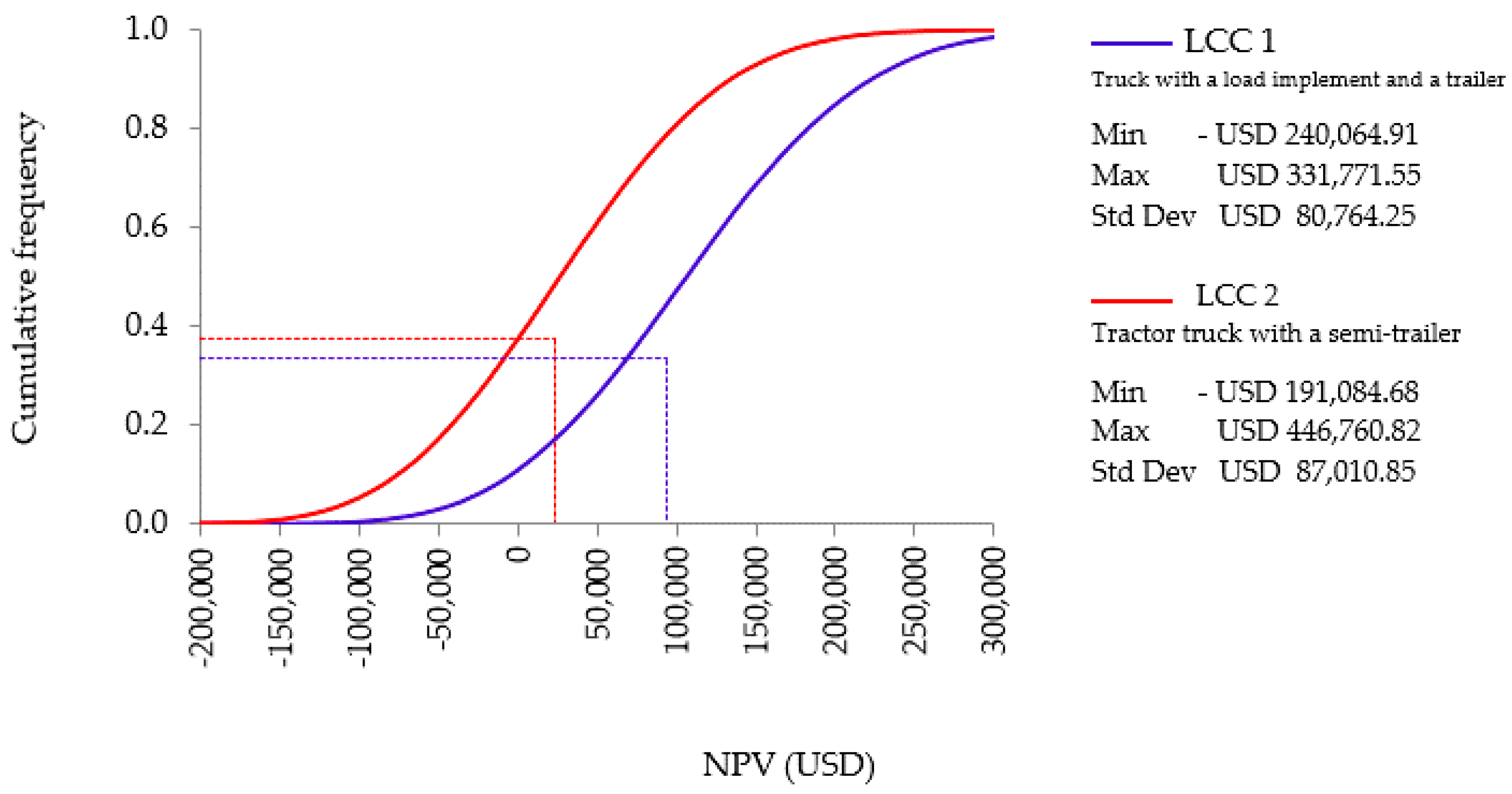
2.4. Investment Project Assessment

The investment project assessment was performed based on the discounted cash flow (DCF) analysis, which considered the annual gross revenue, annual costs, initial investment (value of LCC), corporate income tax (with a tax rate of 25.0% on the earnings before interest and taxes (EBIT)), and disinvestments in fixed assets (LCC). Therefore, the cash flow was considered to be conventional for presenting a single change in sign over the planning horizon of the company, which was six years in accordance with the useful life of the LCCs. Moreover, although the financial investment projects (the two LCCs) have initial capital with different values and the same function, they compete with each other and are mutually exclusive.

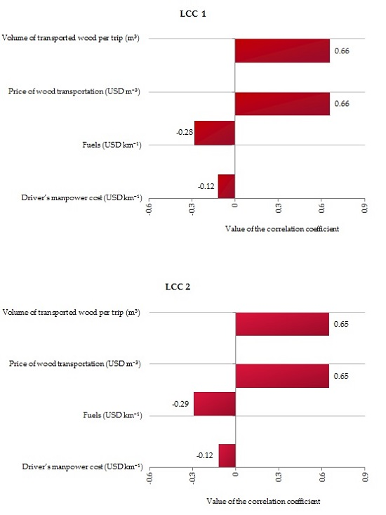
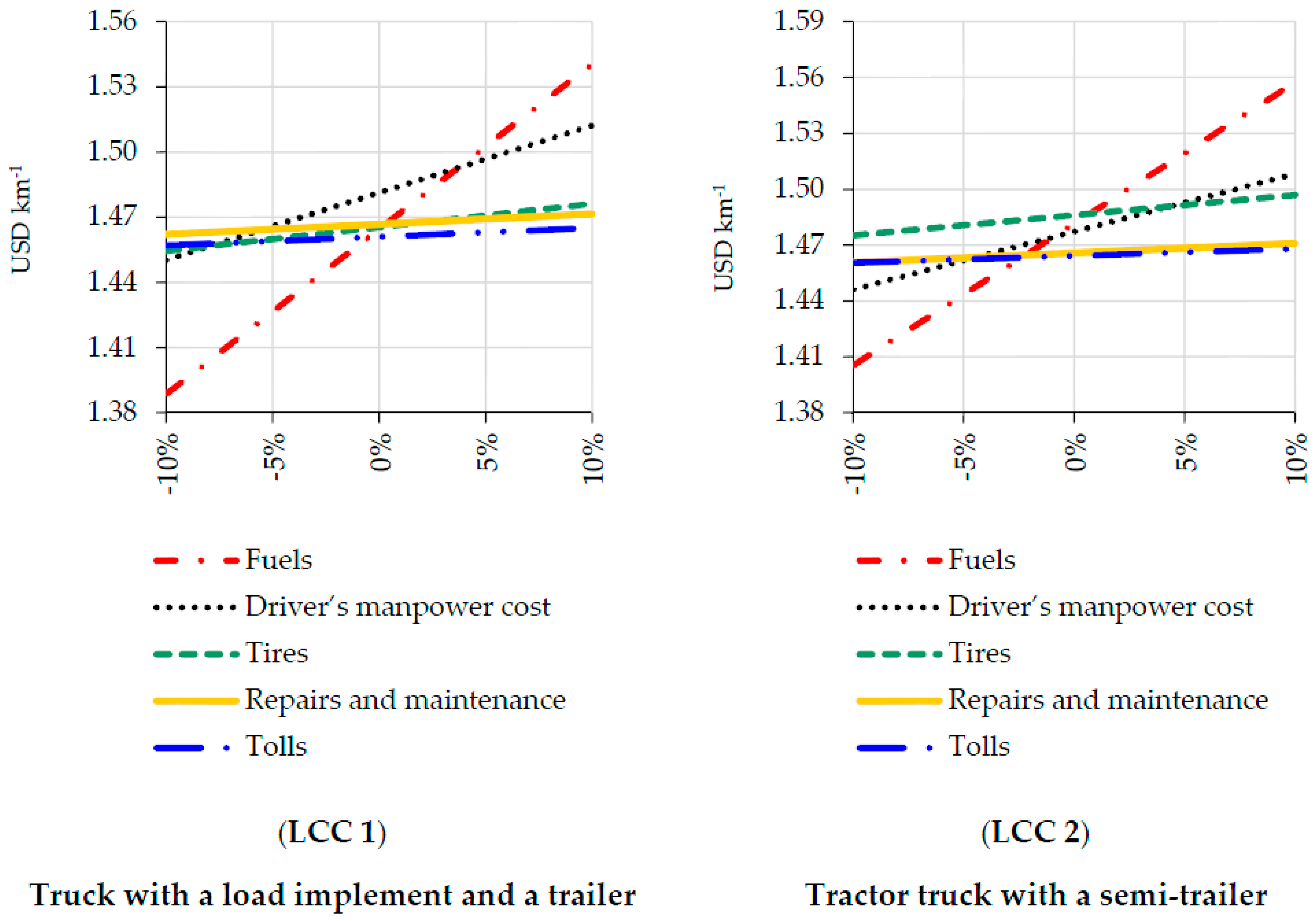
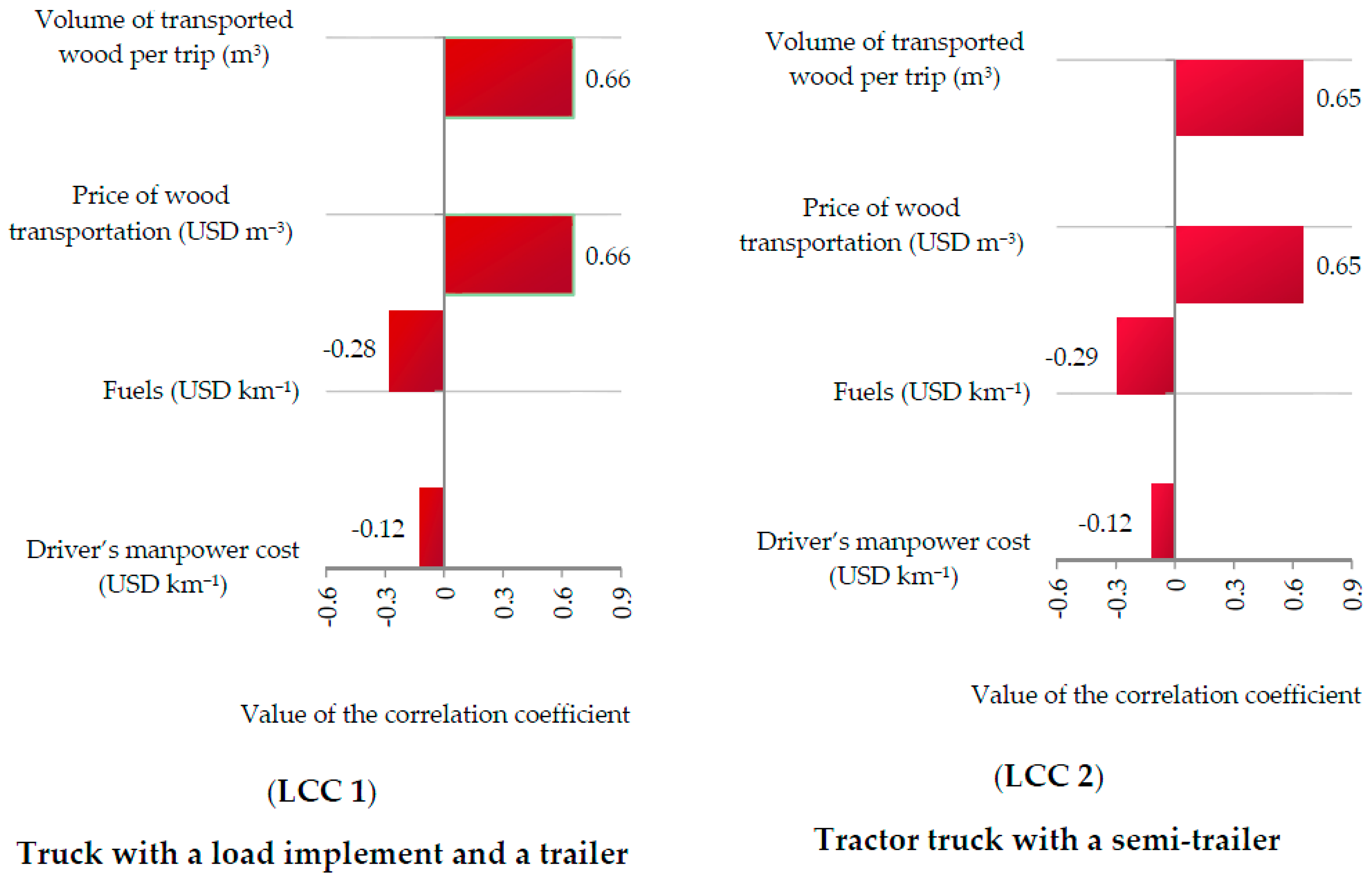
2.5. Risk Analysis of the Investment Project

The addition of risk to the financial investment projects came from the generation of 100,000 pseudorandom numbers by the stochastic Monte Carlo method, with the assistance of the @Risk 6.3.1 software (Copyright © 2014 Palisade Corporation, Ithaca, USA) [21]. The default of the random number generator of the @Risk was the Mersenne Twister, consistent with Matsumoto and Nishimura [22].
The stochastic simulation united the occurrence probability distribution and the correlation between the input variables, and was obtained by means of a non-parametric statistical technique, the Spearman’s rank-order correlation coefficient ρ s , which ranges from −1 to 1 [23].
Based on the established literature, the input variables of the stochastic simulation model were all components of the LCCs’ operational costs (USD km−1), volume of transported wood per trip (m3), price of wood transportation (USD m−3), and acquisition value of the LCCs (USD) [24].
The input variables followed a symmetrical triangular distribution, which had central peak (mode) and endpoints (minimum and maximum). They were easy to understand and commonly used in uncertainty analysis when there was no credible information about the probability distribution of the weighted variables in the stochastic model. Thus, a variant of ±15.0% of the deterministic values was delimited, except for the volume of transported wood per trip (m3), which was designed by the decomposition of time series of the conducted trips.
This decomposition was carried out by the autoregressive integrated moving average process-ARIMA (p.d.q.), commonly used for time series prediction, where p denotes the number of autoregressive terms, d is the number of times that the series must be differentiated before becoming stationary, and q is the number of terms of the moving average [25]. For this procedure, the Box-Jenkins methodology was adopted, along with Bayesian Information Criterium-BIC selection criteria, for allowing the model adjustment and choosing the one that yields the lowest value for the criterion [26,27,28].
The quantitative techniques of economic and financial analysis are characterized as response variables of interest of the investment projects (outputs). One consideration is the variation in cash flows resulting from arbitrary time constraints in decision making. Therefore, a minimum attractive rate of return of 14.0% per year was adopted as a premise and as an indication to investors of the minimum return required to financial investment projects. This reflected the sum of the interest rate adopted by the financial market and the rate risk determined by the investor.
Thus, the Net Present Value (NPV) [29] was used, as it considers the value of money over time. The NPV is particularly notable for being one of the techniques applied in the analysis of financial investment projects, in addition to the Modified Internal Rate of Return (MIRR) [30] and the Profitability Index (PI) [31].

3. Results and Discussion

Uncertainty of cost items is an important aspect of complex projects, and its analysis help decision makers understand and model different factors affecting funding exposure and ultimately estimate the cost of the project [32]. The quantification of these uncertainties is a basic premise to determine the risk of the investment project. This is associated with the probability distribution of each component of the operational cost, because the transportation cost corresponds to a large proportion of the total raw material cost in wood processing plants [3].
One of the main factors that influences the cost of road transportation of wood is the distance between the forest stand and the manufacturing unit that processes the raw material. Thus, for this study, the round-trip distance was 184.4 km, which allowed estimating a modal value for the operational cost of 1.46 USD km−1 for LCC 1 and a modal value of 1.48 USD km−1 for LCC 2. This difference results from divergences in values of fixed assets (LCC) used in the calculation, i.e., the values for the LCC units were 70,208.30 USD and 76,127.29 USD, for LCC 1 and LCC 2, respectively.
Among the components of the operational cost of both LCC, the cost of fuel was the most relevant, with the highest Spearman’s rank-order positive correlation coefficient ( ρ s = 0.91) and the most statistically significant (p-value < 0.0001), followed by the driver’s manpower cost (0.35). Thus, fuel cost has the greatest impact in the cost of road transportation of wood, confirming Freitas et al. [33] in a study that weighed three methodologies for operational cost calculation of trucks used in wood transportation. Figure 1 shows the five most expensive components and their respective impacts due to changes in percentages from the modal values.
The productivity of road transportation of wood can be expressed as the volume of transported wood. Other possibilities, like the amplitude of productivity variation, is considered to be a measure of risk [34,35]. Thus, based on the average of the moving range by the ARIMA process (p.d.q.) and the BIC criterion, a modal value of 30.32 m3 of transported wood per trip was assumed for LCC 1 and 29.72 m3 for LCC 2.
Although the average mass of LCC 1 is 0.29 tons greater than LCC 2, even with an identical MWLA, the difference in wood volume transported per trip may be explained in terms of length, which provided better arrangement of the wood with fewer empty spaces between them after loading in LCC 1, even though the forest tree species, length of the logs, stem conicity, wood density and other factors were similar for both characterizations of the evaluated carrier compositions. The vehicle’s load capacity used for road transportation of wood and losses due to differences in volume, mass and shape of the raw material are the primary factors that influence the final cost of the wood [36,37].
In addition to the difference in the volume of transported wood, there was also a distinction in the duration of activities that comprised the wood transportation and displacement speed of LCC. Accordingly, it was possible to perform 3.8 operating cycles every 24 h with LCC 1 and only 3.5 with LCC 2. The operating cycle time is mainly dependent on the transportation distance and average speed of operation [38]. Therefore, the modal value of the volume of wood (m3) transported annually was 31,680.96 and 29,253.51 for LCC 1 and LCC 2, respectively. As the amount of transported wood increases, there is consequently an increase in gross revenue [39]. Thus, LCC 1 generated more revenue, resulting in a modal value of 352,093.89 USD year−1, while for LCC 2, this value was 313,498.11 USD year−1.
Spearman’s rank-order correlation was used to identify the correlation, both positive and negative, of the most critical variables that influence the NPV of the financial investment projects. This is an important step as it provides elements for strategic diagnosis [40]. Figure 2 shows that for LCC 1, the volume of transported wood (m3) and the average price of wood transportation (USD m−3) have significant positive correlation (p-value < 0.0001) with the NPV: the higher the volume of transported wood, the higher the NPV. This condition is identical to the average price of wood transportation. This situation is similar for LCC 2, corroborating prior research, which showed that the price of wood transportation and volume of transported wood per trip have great influence on the economic-financial viability of wood transportation [41].
The variables of fuel cost, driver’s manpower cost, tire cost, and acquisition value of LCCs also have an inverse relationship with NPV and thus increase the risk level of NPV for both LCCs.
Descriptive statistics are commonly used in research as a basis of analyses and interpretations to represent the results [42]. The results of this analysis showed that the NPV of both LCCs have an approximately normal distribution pattern for presenting asymmetry (0.1) and kurtosis (2.8), which are close to 0 and 3, respectively. These findings are also supported by the proximity of the median to the mean and modal values [43].
An important criterion to evaluate an investment project is its NPV. However, this needs information on the robustness of the result to support the decision makers during their assessment of the risk of the project [44]. The concept of risk is conventionally framed in terms of a divergence between an expected outcome and an adverse result, with respect to some phenomenon of interest [45]. By analyzing the cumulative frequency of the NPV (Figure 3) generated by LCC 1, it is possible to determine that this divergence is 33.5%, considering that the modal value of the NPV is 93,812.27 USD. In relation to LCC 2, this frequency identifies that there is a 37.5% probability that this investment analysis technique will yield an adverse outcome, considering the modal value of 23,216.91 USD.
One of the conditions used to demonstrate the attractiveness of a project is to identify the individual risks that impact the cash flow of the financial investment project [46]. These risks can be analyzed through sensibility analysis that plays an important role in scenario reasoning, and hence decision making [47]. Thus, when considering a reduction of 5.0% in the volume of transported wood per trip (m3), which can be considered the most critical variable of the investment project, there will be an average increase in the risk of the investment projects of 6.9%, which would make the use of LCC 2 uneconomical because the result would be a negative NPV.
The method modified internal rate of return (MIRR) has been suggested to resolve the problems arising from the reinvestment assumption of the cash flow [48]. Therefore, a minimum attractive rate of return (cost of capital of the company) was assumed to reinvest the positive cash flows and the financial market rate for fixed income securities of 7.5%, paid on the monetary values used in negative cash flows. The MIRR modal value for LCC 1 was 35.0%, although there is a risk of 14.1% that this rate results in a percentage equal to or below the minimum rate of attractiveness. When analyzing LCC 2, this risk was 10.4% for a modal value of 29.1%.
The profitability index (PI) identifies the relationship between expenses and the profit of the proposed system as a ratio [49]. Thus, a probabilistic profitability index analysis is also conducted to address the potential economic risk, and the results provide an accurate indication of the return period over the investment period [50]. This analysis determines that for LCC 1, there is a risk of 11.0% that the index is less than zero when considering a modal value of 2.76. In other words, this risk may be considered low, especially when expecting that this project will produce 1.76 USD of this value for each USD invested. On the other hand, for LCC 2, this risk is 37.5% considering that the obtained modal value is 1.22 USD. Therefore, it will provide a relative profitability of 0.22 USD for the investment project.
Mathematically, the used financial analysis techniques can create conflicts for mutually exclusive projects [24] that are having scaling problems. Thus, although the LCC 2 investment project is higher (initial investment) when compared to LCC 1 (lower initial investment), the results do not produce conflicts, indicating that LCC 1 provides a better return on invested capital because the invested values for all analysis techniques were superior to those found for LCC 2, even considering that the NPV is an absolute value.

4. Conclusions

The methodology used to estimate the operational cost allowed us to closely approximate the actual values, because it included cost components that are not weighted in methodologies commonly used by the wood processing plants.
The costs of fuel, driver manpower and tires are the most critical components of the operational costs, as they increase the level of financial risk, and may derail the investment in road transportation of wood.
The investment projects in LCC used for road transportation of wood in Uruguay are influenced by the variation effect of the volume of transported wood and cost of wood transportation, resulting in an average risk of 35.5% that the NPV is less than zero.
For the condition studied, MIRR demonstrated that the road transportation of wood provides an average return of 18.0% on the minimum attractive rate of return determined by the investor, associated with an average risk of 12.3%.

Acknowledgments

This work was supported by Coordenação de Aperfeiçoamento de Pessoal de Nível Superior (CAPES).

Author Contributions

Danilo Simões designed the methodology, did most of the data-analysis, wrote the paper and guided manuscript writing and editing; Gustavo A. Daniluk Mosquera conceived the experiment; Gislaine C. Batistela contributed to methodology and discussion sections; José R. de S. Passos gave ideas for study and processed some data; Paulo T. Fenner coordinated the study.

Conflicts of Interest

The authors declare no conflict of interest.

References

  1. Machado, C.C.; Lopes, E.S.; Birro, M.H.B. Transporte Rodoviário Florestal, 2rd ed.; UFV: Viçosa, Brasil, 2009; pp. 1–167. [Google Scholar]
  2. Hakkila, P. Procurement of Timber for the Finnish Forest Industries; Finnish Forest Research Institute: Vantaa, Finland, 1995; pp. 1–73. [Google Scholar]
  3. Frisk, M.; Göthe-Lundgren, M.; Jörnsten, K.; Rönnqvist, M. Cost allocation in collaborative forest transportation. Eur. J. Oper. Res. 2010, 205, 448–458. [Google Scholar] [CrossRef]
  4. Carlsson, D.; Rönnqvist, M. Supply chain management in forestry-case studies at Södra Cell AB. Eur. J. Oper. Res. 2005, 163, 589–616. [Google Scholar] [CrossRef]
  5. Berger, R.; Timofeiczyk, R., Jr.; Carnieri, C.; Lacowicz, P.G.; Junior, J.S.; Brasil, A.A. Minimização de custos de transporte florestal com a utilização da programação linear. Rev. Flor. 2005, 33, 53–62. [Google Scholar] [CrossRef]
  6. Food and Agriculture Organization. The Cost of Truck Transport for Wood in Some European Countries; Food and Agriculture Organization: Rome, Italy, 1969; pp. 1–17. [Google Scholar]
  7. Strehlke, B. Anweisung zur Herleitung von Maschinenbetriebskosten in der Forsfwirtschaft, 1st ed.; Kuratorium für Waldarbeit und Forsttechnik: Buschlag, Germany, 1971; pp. 1–12. [Google Scholar]
  8. Berger, R. Minimização do Custo de Transporte de Madeira de Eucalipto no Estado de São Paulo. Master’s Thesis, Universidade de São Paulo, São Paulo, Brazil, 1975. [Google Scholar]
  9. Watanatada, T.; Paterson, W.D.O.; Bhandari, A.; Harral, C.; Dhareshwar, A.M.; Tsunokawa, K. The Highway Design and Maintenance Standards Model: Description of the HDM-III Model; World Bank: Washington, DC, USA, 1987; pp. 149–236. [Google Scholar]
  10. SAAB-SCANIA do Brasil Ltda. Custos Operacionais; Centro Gráfico SAAB-SCANIA: São Bernardo do Campo, Brasil, 1988; pp. 1–68. [Google Scholar]
  11. Machado, C.C. Sistema Brasileiro de Classificação de Estradas Florestais (SIBRACEF): Desenvolvimento e Relação com o meio de Transporte Florestal Rodoviário. Ph.D. Thesis, Universidade Federal do Paraná, Paraná, Brazil, 1989. [Google Scholar]
  12. Jokic, S.V.; Zupunski, L.; Zupunski, I. Measurement uncertainty estimation of health risk from exposure to natural radionuclides in soil. Measurement 2013, 46, 2376–2383. [Google Scholar] [CrossRef]
  13. Hilli, P.; Koivu, M.; Pennanen, T. Cash-flow based valuation of pension liabilities. Eur. Actuar. J. 2011, 1, 329–343. [Google Scholar] [CrossRef]
  14. Scott, D.F.; Moore, L.J. Financial planning in a simulation framework vectors. Atlanta Econ. Rev. 1975, 10–14. [Google Scholar]
  15. Hertz, D.B.; Thomas, H. Risk Analysis and its Applications; Wiley: Chichester, UK, 1983; pp. 11–15. [Google Scholar]
  16. Mattos, A.C.M.; Vasconcellos, H. Análise de sensibilidade. Rev. Adm. Empres. 1989, 29, 85–91. [Google Scholar] [CrossRef]
  17. Danh, V.T.; Khai, H.V. Using a Risk Cost-Benefit Analysis for a Sea Dike to Adapt to the Sea Level in the Vietnamese Mekong River Delta. Climate 2014, 2, 78–102. [Google Scholar] [CrossRef]
  18. Tsu-Ming, Y.; Jia-Jeng, S. Preventive maintenance model with FMEA and Monte Carlo simulation for the key equipment in semiconductor foundries. Sci. Res. Essays 2011, 6, 5534–5547. [Google Scholar] [CrossRef]
  19. Safadi, E.A.E.; Adrot, O.; Flaus, J.M. Advanced Monte Carlo Method for model uncertainty propagation in risk assessment. IFAC Pap. 2015, 48, 529–534. [Google Scholar] [CrossRef]
  20. Banco Central del Uruguay. Available online: http://www.bcu.gub.uy/Estadisticas-e-Indicadores/Paginas/Cotizaciones.aspx (accessed on 28 February 2016).
  21. Palisade Corporation. @Risk for Excel. v. 6.3.0; Palisade Corporation: Ithaca, USA, 2014. [Google Scholar]
  22. Matsumoto, M.; Nishimura, T. Mersenne twister: A 623-dimensionally equidistributed uniform pseudo-random number generator. ACM Trans. Model. Comput. Simul. 1998, 3, 3–30. [Google Scholar] [CrossRef]
  23. Spearman, C. “General Intelligence,” Objectively Determined and Measured. Am. J. Psychol. 1904, 15, 201–292. [Google Scholar] [CrossRef]
  24. Brigham, E.F.; Ehrhardt, M.C. Financial Management: Theory and Practice, 14th ed.; Cengage Learning: Kentucky, USA, 2014; pp. 415–459. [Google Scholar]
  25. Gujarati, D.N.; Porter, D.C. Basic Econometrics, 5th ed.; McGraw-Hill Companies: New York, NY, USA, 2011; pp. 767–793. [Google Scholar]
  26. Box, G.E.P.; Jenkins, G.M.; Reinsel, G.C. Multivariate Time Series Analysis, 4th ed.; John Wiley & Sons, Inc.: Hoboken, NJ, USA, 2008; pp. 551–595. [Google Scholar]
  27. Schwarz, G. Estimating the dimension of a model. Ann. Stat. 1978, 6, 461–464. [Google Scholar] [CrossRef]
  28. Paula, P.W.; Lima, G.B.; Zanetti, J.B. Análise comparativa de modelos de séries temporais para modelagem e previsão de regimes de vazões médias mensais do Rio Doce, Colatina-Espírito Santo. Cienc. Nat. 2015, 37, 1–11. [Google Scholar]
  29. Źróbek-Różańska, A.; Nowak, A.; Nowak, M.; Źróbek, S. Financial Dilemmas Associated with the Afforestation of Low-Productivity Farmland in Poland. Forests 2014, 5, 2846–2864. [Google Scholar] [CrossRef]
  30. Kierulff, H. MIRR: A better measure. Bus. Horiz. 2008, 51, 321–329. [Google Scholar] [CrossRef]
  31. Swalm, R.O. Profitability index for investments. Eng. Econ. 1958, 3, 40–46. [Google Scholar] [CrossRef]
  32. Khodakarami, V.; Abdi, A. Project cost risk analysis: A Bayesian networks approach for modeling dependencies between cost items. Int. J. Proj. Manag. 2014, 32, 1233–1245. [Google Scholar] [CrossRef]
  33. Freitas, L.C.; Marques, G.M.; Silva, M.L.; Machado, R.R.; Machado, C.C. Estudo comparativo envolvendo três métodos de cálculo de custo operacional do caminhão bitrem. Rev. Árvore 2004, 22, 855–863. [Google Scholar] [CrossRef]
  34. Andreu, L.; Gutiérrez, E.; Macias, M.; Ribas, M.; Bosch, O.; Camarero, J.J. Climate increases regional tree-growth variability in Iberian pine forests. Glob. Chang. Biol. 2007, 13, 804–815. [Google Scholar] [CrossRef]
  35. Tilman, D.; Knops, J.; Wedin, D.; Reich, P.; Ritchie, M.; Siemann, E. The influence of functional diversity and composition on ecosystem processes. Science 1997, 277, 1300–1302. [Google Scholar] [CrossRef]
  36. Alves, R.T.; Fiedler, N.C.; Silva, E.N.; Lopes, E.S.; Carmo, F.C.A. Análise técnica e de custos do transporte de madeira com diferentes composições veículares. Rev. Árvore 2013, 37, 897–904. [Google Scholar] [CrossRef]
  37. Hederstrom, T. Ubicación de las Industrias Forestales; FAO: Rome, Italy, 1974; pp. 1–11. [Google Scholar]
  38. Machado, R.R.; Silva, M.L.; Machado, C.C.; Leite, H.G. Avaliação do desempenho logístico do transporte rodoviário de madeira utilizando rede de petri em uma empresa florestal de Minas Gerais. Rev. Árvore 2006, 30, 999–1008. [Google Scholar] [CrossRef]
  39. Lacowicz, P.G.; Berger, R.; Júnior, R.T.; Silva, J.C.G.L. Minimização dos custos de transportes rodoviário florestal com o uso da programação linear e otimização do processo. Floresta 2002, 32, 75–87. [Google Scholar] [CrossRef]
  40. Rodrigues, A.; Rojo, C.A.; Bertolini, G.R.F. Formulação de estratégias competitivas por meio de análise de cenários na construção civil. Produção 2013, 23, 269–282. [Google Scholar] [CrossRef]
  41. Silva, M.L.; Oliveira, R.J.; Valverde, S.R.; Machado, C.C.; Pires, V.A.V. Análise do custo e do raio econômico de transporte de madeira de reflorestamentos para diferentes tipos de veículos. Rev. Árvore 2007, 31, 1073–1079. [Google Scholar] [CrossRef]
  42. Zaidan, A.; Ismail, Z.; Yusof, Y.M.; Kashefi, H. Misconceptions in Descriptive Statistics among Postgraduates in Social Sciences. Soc. Behav. Sci. 2012, 46, 3535–3340. [Google Scholar] [CrossRef]
  43. Black, F.; Scholes, M. The pricing of options and corporate liabilities. J. Political Econ. 1973, 81, 637–654. [Google Scholar] [CrossRef]
  44. Van Groenendaal, W.J.H. Estimating NPV variability for deterministic models. Eur. J. Oper. Res. 1998, 16, 202–213. [Google Scholar] [CrossRef]
  45. Inanoglu, H.; Jacobs, M. Models for Risk Aggregation and Sensitivity Analysis: An Application to Bank Economic Capital. J. Risk. Financ. Manag. 2009, 31, 118–189. [Google Scholar] [CrossRef]
  46. Arnold, U.; Yildiz, Ö. Economic risk analysis of decentralized renewable energy infrastructures—A Monte Carlo Simulation approach. Renew. Energy 2015, 77, 227–239. [Google Scholar] [CrossRef]
  47. Yang, J. Convergence and uncertainty analyses in Monte-Carlo based sensitivity analysis. Environ. Model. Softw. 2011, 26, 444–457. [Google Scholar] [CrossRef]
  48. Satyasai, K.J.S. Application of Modified Internal Rate of Return Method for Watershed Evaluation. Agric. Econ. Res. Rev. 2009, 22, 401–406. [Google Scholar]
  49. Baral, S.; Kim, K.C. Stand-alone solar organic rankine cycle water pumping system and its economic viability in Nepal. Sustainability 2015, 8, 1–18. [Google Scholar] [CrossRef]
  50. Sajid, Z.; Zhang, Y.; Khan, F. Process design and probabilistic economic risk analysis of bio-diesel production. Sustain. Prod. Consum. 2016, 5, 1–15. [Google Scholar] [CrossRef]
Figure 1. Modal value of the operational cost of transportation (USD km−1) versus the percentage change of the most relevant components.
Forests 07 00130 g001
Figure 2. Spearman’s rank-order correlation coefficient of the most critical input variables of the stochastic simulation model in relation to the simulated NPV of financial investment projects of road transportation of wood.
Forests 07 00130 g002
Figure 3. Cumulative frequency of the simulated NPV for the financial investment projects of road transportation of wood.
Forests 07 00130 g003

