A Linear Programming Model to Biophysically Assess Some Ecosystem Service Synergies and Trade-Offs in Two Irish Landscapes

Abstract

Ecosystem service provisions are becoming more frequently used to assess land-use related conflicts in recent decades. This study investigates the current spatial and research information available to quantify ecosystem services relative to forest land-use planning in Ireland. A model is developed using the linear-programming method in Remsoft’s Woodstock platform. This model is applied to two case study areas in Ireland: Western Peatlands and Newmarket. Each case study area was chosen to assess a unique issue in the Irish and European context on the provision of ecosystem services. Western Peatlands was chosen to assess the effects of forest and alternative land-use options and Newmarket was chosen to investigate the effect of afforestation. The synergies and trade-offs of biophysically optimising the provisions of each ecosystem service are presented and discussed. The study quantitatively determines that trade-offs among provisions of some ecosystem services are required when optimising an ecosystem service while other ecosystem services are synergistic when the provision of a single ecosystem service is optimised.

1. Introduction

Deforestation, relating to land settlement and Ireland’s colonial past, resulted in a forest cover of circa 1% around the beginning of the 20th century. The most recent National Forest Inventory was carried out in 2012 and estimated the total forest cover to have increased to approximately 10.5% [1]. Coillte (the Irish State Forestry Board, Newtownmountkennedy, Ireland), owns circa 53% of this, with the remainder owned by private landowners (ibid). Forests, public and private, have typically been planted on marginal land (Not suitable for agriculture but suitable for forestry) since the middle of the 20th century. As this marginal land is not suitable to grow high quality broadleaves, the majority of Irish forests comprise (exotic) conifers such as Sitka spruce (Picea sitchensis (Bong.) Carr), lodgepole pine (Pinus contorta) and Norway spruce (Picea abies (L.) H. Karst). These three species make up approximately two-thirds of the Irish forest estate [1]. However, many areas of Ireland have the biophysical potential for a range of land-uses and tree species.

Studies in a forestry context have suggested that proper sustainable forest management (SFM) will depend on the balance between its three pillars (environmental, social and economic) and their indicators [2,3,4]. Ecosystem services (ES) are a utilitarian concept which may prove useful to identify this balance [5]. A full history of the evolution of the ES concept is described by [6]. Briefly, the origin of the concept dates back to the late 1960s [7]. It was used in the 1970s to capture public interest in terms of biodiversity conservation [8]. Since then, the number of academic publications referring to the term ESs has gradually increased culminating in the Millennium Ecosystem Assessment; a major piece of work which provided an indication of the level of degradation of the world’s ESs [9]. Quantifying ESs would make it possible to evaluate trade-offs and compatibility of ESs between different management scenarios in a given landscape. However, debate continues about the most appropriate method to define and quantify ESs with consistency. It is broadly accepted that localised studies will provide a more accurate assessment of ESs than on the global scale [10]. Managing for the provision of multiple ESs is one of the key challenges of ecosystem provision and state that trade-offs and synergies of ESs are particularly significant issues in addressing this at the landscape level [11]. DeGroot, et al. [12] have suggested indicators that link ESs to human well-being. In Ireland, political attention has focused on specific ESs, and land-use disputes have identified ESs that are strongly related to human welfare. Research in Ireland has investigated these [13,14,15,16] and most of the relevant ESs can be summarised into the categories outlined by DeGroot, Alkemade, Braat, Hein and Willemen [12].

Since the 1960s, many forests in Ireland have been established with a focus on generating revenue and this remains the main objective generally. This single financially oriented objective has guided forest decision support system (DSS) research in Ireland in the past. Nieuwenhuis and Williamson [17] developed a system for timber harvesting and sawmill delivery while minimising costs. More recently, SFM has come to the fore in Irish forest management and research effort has shifted. Forest research effort has become less focused on timber production with more of an emphasis now being placed on forests’ non-timber benefits in parallel with timber supply, ESs. The potential to optimally group sub-compartments (the smallest unit of management used by Coillte) to create economically viable blocks for harvesting was explored by Nieuwenhuis and Tiernan [3]. They went on to implement some SFM constraints and compared their economic impact. PractiSFM, a simulation based DSS was developed to provide an approach for private forest owners to compile and forecast various management prescriptions while viewing the associated trade-offs of a range of ESs [2].

The objective of this study is to develop a DSS to quantify and evaluate the trade-offs of ES provisions at the landscape level over the course of a 70-year planning horizon, beginning in 2012. As forest rotations in Ireland are mostly 35 to 45 years, a 70-year planning horizon is sufficient to capture the full ES provision cycle. By using two Case Study Areas (CSAs) (i.e., the Western Peatlands and Newmarket) in which the developed model was applied, an indication of ES provision potential will be obtained given the specific biophysical conditions in each CSA, while excluding Irish forest policy, regulation and industry demand requirements. These provision levels will provide the production frontiers for each ES in each CSA, while the effect of optimising one ES on the provision levels of the other ESs will give an indication of their compatibility.

In order to investigate the long-term future of forest growth and the associated ES provision, planning on a strategic time scale is required. The linear programming (LP) component of Remsoft (Woodstock) (Remsoft, 2014.07, Fredericton, New Brunswick, Canada) was chosen as the most suitable tool to investigate the provision of ESs in the fragmented and complex landscapes chosen for this study. Optimisation will deliver the preferred management prescriptions available and will identify ES production frontiers, trade-offs and synergies associated with these prescriptions. Access to the Remsoft software in both the academic and industrial partners in the project facilitated the development of the model through the exchange of spatial and management information.

2. Materials and Methods

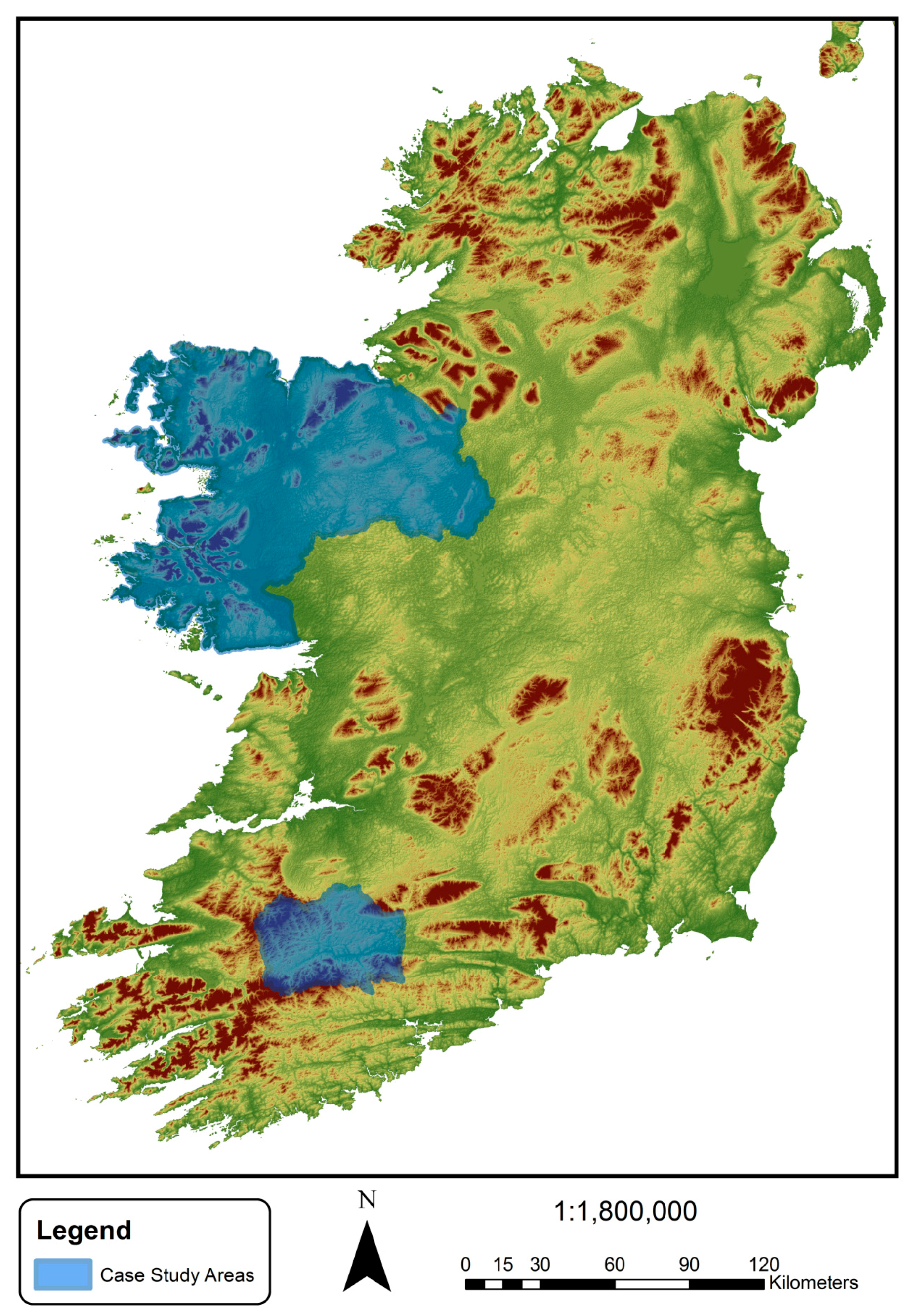
2.1. Description of CSAs

2.1.1. Western Peatlands

The Western Peatlands (WP) CSA is located in the northwest of Ireland (Figure 1). It is based on a Business Area Unit, a method of land division and management used by Coillte. There are eight Business Area Units in the Republic of Ireland. Their boundaries follow town land boundaries (as much as possible) and they were designed to be independently profitable units [18]. The location of the WP CSA means that wind exposure is a dominant factor for all land-use options. The east of the CSA is more fertile and has more potential for land-use applications than the west which enables the potential for a range of agricultural land-uses, i.e., dairying and beef production. However, afforestation on these better soils is a much smaller political issue in this CSA than the management of the forested peatlands.

2.1.2. Newmarket

The Newmarket (NM) CSA takes in the north of county Cork (Figure 1). The central part of the CSA, known as the Duhallow region, is designated as a disadvantaged area vis-à-vis the allocation of EU structural funds. Dairying is the major farm enterprise in the NM CSA. Tillage is also quite substantial, but is confined to the most fertile sites in the eastern parts of the CSA. There are strong regional variations in terms of farm scales and incomes. Farms located at lower elevations that are mainly specialising in dairying and tillage production tend to be bigger and more economically viable than smaller farms located in the hills that rely on cattle and sheep farming. Forests are almost exclusively located in the less fertile, upland areas of the CSA. Considering that afforestation will be investigated in this CSA, both forestry and agricultural land is included. Statistics that provide a description of each CSA are provided in

Table 1. Statistics associated with the Western Peatlands and Newmarket case study areas.

-	Western Peatlands	Newmarket
Area (approximately in ha)	1,060,000	188,000
Forested area (approximately in ha)	116,000	32,000
Average temperature (°C)	11–12	8–9
Typical annual rainfall (mm)	West: 2000	1200–1400
	East: 1200–1400
Forested land only (as of 2012)
Forest ownership
Coillte	64%	68%
Private	36%	32%
Yield potential
Productive forestry	82%	85%
Unproductive forestry	18%	15%
Age class distribution 0–10 years	26%	14%
11–20 years	36%	36%
21–30 years	19%	28%
31–40 years	13%	14%
41–50 years	5%	6%
51 years or over	1%	2%
Soil type
Brown earths and brown podzolics	5%	58%
Lithosols	12%	9%
Gleys/peaty gleys and gleyed grey brown podzolics	17%	26%
Flushed blanket peat	48%	7%
Cutaway raised bogs	18%	0%
Elevation
Less than 200 m	93%	26%
Distance to watercourse
Less than 200 m	56%	27%
Between 200 and 400 m	26%	28%
400 m or greater	19%	45%

Forestry that has a Sitka spruce yield class equivalent of 14 or higher is considered to be economically viable and hence productive [19].

.

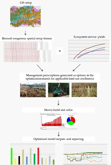
2.2. Decision Support System and Model

The model was developed in Remsoft, a Canadian developed software package. Woodstock [20] accommodates linear programming and uses an exogenous modelling method, meaning that spatial constraints are determined before the optimisation takes place. It is intended for long-term strategic planning, based on input in the form of ESRI shape files (ESRI, Redlands, CA, USA), ESRI geodatabases or database files. This methods section will focus on the data and data manipulation required to develop and implement the model in Woodstock’s linear programming structure. Woodstock builds a matrix in a mathematical programming system, which is solved using the MOSEK mathematical programming solving software. This study used Windows (Microsoft, Redmond, Washington, WA, USA) 7 Professional 64 bit (SP1) operating system with an Intel^® Core™ i7-3930K CPU @ 3.20 GHz (6 cores with 2 threads per core) PC with 32 GB of RAM.

2.3. Coillte Collaboration

Coillte developed a Remsoft based, country-wide timber harvesting model. The objective of this model is to maximise Net Present Value (NPV) from the harvesting and delivery of timber products to mill gate, while encompassing access, ecological and environmental constraints in the form of financial disincentives. The financial objective of Coillte’s model stems from its commercial mandate. The company provided this base model (in February 2012) for use in this study.

2.4. Remsoft Model Setup

There are three bodies of work required in order to produce a functioning model for Remsoft Woodstock (Figure 2): Management prescriptions (Section 2.4); GIS setup and spatial setup in Remsoft (Section 2.5); and Ecosystem Service yields and forest inventory attributes (Section 2.6). Each element requires its own setup prior to implementation. The model accommodates a maximum of three forest species per polygon.

2.5. Management Prescriptions

Management prescriptions are choices available to the model. The range of choices available depends on site and stand conditions. These prescriptions include retention, site preparation, fertilising, forestation, thinning (including continuous cover forestry (CCF)) and clearfelling operations (

Table 2. Forest management prescriptions available in the model.

Management Prescription	Site and Stand Condition(s) for Eligibility of Management Prescription
Retention	No anthropogenic intervention takes place. Forests are allowed to mature until the next year of the model.
	Site Preparation
Mounding	A requirement to prepare a site for establishment on infertile peats. Not prescribed to native woodland sites.
Fencing	An entire site was fenced for afforestation and half of this cost was assumed for fence maintenance at reforestation. This is based on area rather than perimeter.
Fertilising	Sites which have supported a previous yield class of 14 m3·ha−1·year−1 or less for conifers, or 6 m3·ha−1·an−1 or less for broadleaves, receive 2 fertilisation applications (one at establishment and one at year 5) to ensure establishment. Sites whose forest productivity needs to be determined (i.e., agricultural sites) were assessed for fertilisation based on a fertility model adapted from Farrelly, et al. [21].
	Forestation
	The grant premium categories for afforestation as outlined by the Irish Forest Service in 2012 were used for afforestation and reforestation (reforestation was not grant aided although the options provide a suitable variety of restocking options); with the addition of a reforestation option for WP. Species suitability was determined based on soil type and elevation. Any species with a moderate to optimal suitability for a particular soil type according to Horgan, et al. [22] was considered suitable to be planted under the soil type criterion. Species which had a tolerance of 3–5 according to Horgan, Keane, McCarthy, Lally and Thompson [22] were considered suitable for elevations up to 150 m for broadleaves and 200 m for conifers, while species tolerant of exposure (a rating of 2 or less) were also considered suitable for elevations up to 300 m. Only lodgepole pine (Pinus contorta) was considered suitable for elevations above 300 m for the purpose of reforestation. It is assumed that weevil and vegetation control is applied to all sites on which forest is established (afforestation or reforestation) and that these sites are manually inspected by a forester to ensure that establishment has been successful.
Native woodland	Species selection is based on a site’s soil type as describe in Forest Service [23]; a site must be capable of growing trees without the requirement for fertilisation at establishment.
	Harvesting
	The species with the highest productivity dictates the thinning regime. Conifer stands must be suitably productive for thinning to be an option (i.e., YC ≥ 10). Conifers can begin thinning on a 5-year cycle (for a total of two or four thinnings) at the age of 16 or 22 years (the optimisation chooses the optimal). The thinning interval and potential start ages for broadleaves is YC specific. For a broadleaf species with a YC of 12, thinning takes place at 5 years intervals starting ages of 10 or 16, YC of 10: 10 years intervals starting at ages 12, 20 or 23, YC of 8: 15 years intervals starting at ages 20 or 25, YC of 6: 20 years intervals starting at ages 23, 28 or 33 and YC of 4: 25 years intervals starting at ages 30, 40 or 45. Thinning for CCF can begin at the age of 19 or 42 years (both ages are choices in for the optimisation) and thinnings take place at 5-year intervals for the duration of the planning period.
Clearfell	Clearfelling is an option when the species in a stand with the highest proportion of area is a conifer and exceeds 18 m in mean height or if the species is broadleaf and its age is ≥ 60 years.
	Agricultural Land-Use
	The agricultural land-use and the associated practices are maintained, i.e., ruminant or tillage production (Newmarket only).

).

2.6. GIS Setup

The spatial information is interpreted by Remsoft in a shapefile format. The spatial information and sources required to produce the shapefile for this study are presented in

Table 3. List of GIS layers and their sources.

GIS Layer(s)	Source
Coillte Sub-Compartments	Coillte
Coillte Forests and Old Woodland Sites	Coillte
County Council Roads (Data Collected by Coillte)	Coillte
Wind Zones	Coillte
Irish Land Divisions	Central Statistics Office
Electoral Divisions	Central Statistics Office
Single Farm Payment (SFP) Land Parcels	Department of Agriculture Food and the Marine
Rivers, Lakes and Ponds	Environmental Protection Agency
Teagasc Soil Survey	Environmental Protection Agency
Catchments and Sub-Catchments	Environmental Protection Agency
Private Forests (Forestry07)	Forest Service
Natura 2000 and Native Woodland Sites	National Parks and Wildlife Service
Digital Terrain Model	University College Dublin Urban Institute

. The land-use datasets (i.e., the GIS vector layers that contain the Coillte forest, private forest and agricultural land) were merged in order to produce the land-use layer for this study. Then, GIS techniques and data related queries carried out in ArcGIS 10.1 (ESRI, Redlands, CA, USA) and Microsoft Access 2010 (Microsoft, Redmond, Washington, WA, USA), respectively, were used to assign the necessary attributes to each polygon in the land-use layer.

2.7. Quantifying Ecosystem Service Provision Levels

The origins of the values used in the model for growth, yield, habitat and sustainability parameters are described in this section, as well as their association with various management activities and states of the forest. Details of the metrics used to quantify ecosystem services are provided in Appendix (

Table A7. Species aggregated into groups for the purpose of assigning red squirrel habitat suitability scores.

Aggregate	Species
Small seeded broadleaves	Alder	Ash	Sycamore	Birch	Norway maple
	Salix sp.	Poplar	Rowan	Hornbeam
Big seeded broadleaves	Cherry	Beech	Hazel	Oak	Spanish chestnut
JL	Hybrid larch	Japanese larch	Lawson cypress	Western hemlock	Western red cedar	European larch
NS	Douglas fir	Noble fir	Grand fir	Norway spruce	Other conifer
LP	Corsican pine	Lodgepole pine
SS	Sitka spruce
SP	Scots pine

,

Table A8. Red squirrel habitat suitability scores, by species and age class.

Age Range	Conifers					Broadleaves
(years)	SS	NS	SP	LP	JL.	SSBL	BSBL
0–14	1.00	1.00	1.00	1.00	1.00	1.00	1.00
15–20	1.00	1.00	4.00	4.00	3.00	4.00	1.00
21–30	1.00	1.00	4.00	4.00	4.00	6.00	1.00
31–40	1.00	4.00	5.00	5.00	4.00	6.00	1.00
41–50	2.00	5.00	7.00	8.00	5.00	5.00	3.00
51–60	1.00	6.00	10.00	7.00	5.00	5.00	3.00
61–80	1.00	5.00	10.00	7.00	4.00	5.00	3.00
>80	1.00	5.00	10.00	7.00	4.00	5.00	4.00

,

Table A9. Agricultural (grassland and tillage) and non-forest biodiversity scores post scaling (including the deer forage adjustment).

	Land-Use	NB	GV	DF	DC	RS	HH
Non-forest	Scrub	9.17	4.66	4.82	7.14	1.67	10.00
	Bog	5.00	5.33	4.27	4.29	0.00	10.00
	Short rotation coppice	4.17	2.00	3.09	4.29	1.67	0.00
Grassland	Low-intensity grassland	9.17	5.33	4.22	1.43	0.00	9.00
	Intensive grassland	10.00	3.33	6.40	0.71	0.00	3.00
Tillage	Spring cereals	10.00	2.00	2.32	8.57	0.00	10.00
	Winter cereals	8.33	1.33	3.35	10.00	0.00	10.00
	Winter root crops	8.33	1.33	3.33	2.86	0.00	10.00
	Winter sown cover crops	8.33	2.00	3.33	2.86	0.00	10.00

NB = Nesting Birds, GV = Ground Vegetation, DF = Deer Foraging, DC = Deer Cover, RS = Red Squirrel, HH = Hen Harrier.

,

Table A10. Deer foraging and cover habitat suitability scores for broadleaf and conifer, by age classes (10 years for broadleaves, 5 years for conifers). Source: Barrett, et al. [60].

Broadleaf			Conifer
Age Range	Cover	Forage	Age Range	Cover	Forage
0–10	1.43	6.67	0–5	1.43	6.67
11–20	5.71	5.33	6–10	5.71	2.67
21–30	4.29	4.00	10–15	7.14	1.33
41–50	2.86	2.67	16–20	5.71	2.67
51–60	1.43	1.33	21–30	4.29	1.33
61–70	1.43	1.33	31–40	1.43	2.67
71–80	2.86	2.67	41–45	2.86	4.00
81–90	4.29	4.00	46–50	4.29	5.33
91–100	4.29	5.33	51–100	5.71	6.67
111–120	4.29	6.67
121–130	4.29	6.67
131–200	5.71	6.67

,

Table A11. Land-use coefficients for water sedimentation risk calculation.

Land-Use	Co-Efficient	Description
Agricultural land	0.010	Any land used for agriculture (grassland or tillage)
Cleared forest	0.040	Forest sites cleared in the last 4 years, this includes restocked sites and the first two years of afforested sites
Undisturbed forest	0.005	Any existing forest site that is 3 years or older
Scrubland	0.004	Land not used for agriculture or forestry e.g., scrubland or bog

,

Table A12. Forest recreational scores for a range of forest types. Source: Edwards, Jay, Jensen, Lucas, Marzano, Montagné, Peace and Weiss [42]).

	Native Woodland Site			CCF			Plantation Forestry
Age (years)	Conifer	BL	Mixed	Conifer	BL	Mixed	Conifer	BL	Mixed
1 to 5	3.00	3.50	4.00	3.00	3.50	3.50	1.00	2.50	2.50
6 to 15	3.00	6.00	5.00	3.00	5.00	5.00	2.00	3.50	4.00
16 to 50	5.00	8.00	8.00	6.00	7.50	6.50	3.00	5.00	5.00
51 or older	7.00	10.00	9.00	6.50	8.00	8.50	4.50	6.00	6.00

and

Table A13. Summary of recreation scores for non-forest, including the equivalent forest type and forest stage.

Land-Use	Forest Type (Species Type)	Forest Stage	Forest Land-Use Score
Agricultural land (grassland or tillage)	Plantation (BL)	Establishment	2.50
Bufferzone (scrubland)	Native woodland (BL)	Young	6.00
Bog	Native woodland (Mixed)	Young	5.00

).

Potential end uses for timber produced in Ireland are sawlog, firewood, biomass for energy production, or the raw material for the production by Irish-based companies of a variety of panel products (i.e., medium density fibreboard, oriented strand board and moulded door panels). Experience in Ireland suggests that improper site selection, establishment and management will result in the large majority of Irish broadleaf stands not producing quality sawlog. For this reason, all broadleaf harvesting volume was assumed to be sold as firewood. The volumes are based on the static yield tables produced by the British Forestry Commission [24]. Spacing at establishment was fixed depending on species, and yields are dependent on species, yield class and thinning status. Each static yield table includes diameter at breast height (cm), stocking (stems·ha⁻¹) and harvesting volumes (m³·ha⁻¹). Stand growth is quantified in m³·ha⁻¹·year⁻¹.

There is more information available to quantify NPV (€) than any other ES and this is reflected in this study. This section outlines the revenue and costs of the forest and agricultural practices used in the model:

Silvicultural establishment costs (

Table A1. Silvicultural costs (€·ha⁻¹) of various management activities. Source: Coillte.

Management Intervention	Conifer	Broadleaf
Fertilising	69	14
Fencing	89	204
Mounding	435	409
Planting	800	1108
Weevil control	211	41
Vegetation control	228	376
Inspection	10	10
Road maintenance	1.50€·m−3

): It is assumed that all stands have suitable access for timber extraction and transportation, therefore a road construction cost is not included. However, road maintenance, repair and upgrade costs are included and were assumed to be incurred at a rate of €1.50 per cubic metre harvested in clearfell or thinning.

Annual afforestation premiums (

Table A2. Grant premium categories (GPC) and annual premiums in 2012. Source: Forest Service [52].

GPC	Title	€·ha−1·year−1
3	10% diverse	427
4	Diverse	454
5	Broadleaf	481
6	Oak	515
7	Beech	515
8	Alder	481

).

Forest products the harvested volumes (

Table A3. Forest product prices (standing) used. Source: Coillte.

Product	Price (€·m−3)
Pulp	26
Stake	41
Small sawlog	53
Large sawlog	61
Firewood (broadleaf)	42

): Divided into assortments using an assortment table based on average DBH ([25] Revenue from the sale of standing timber is then calculated based on the constant market price for each product.

Agricultural gross margin (

Table A4. Agricultural financial values used per land-use category. Source: Teagasc National Farm Survey 5-year average gross margin from year 2007 to 2011 inclusive [53,54,55,56,57].

Land-Use Category	€·ha−1·year−1
Mixed livestock
Marginal	415
Profitable	885
Tillage land	979

): The marginal group was assumed to be located on farms designated as hill farms according to Teagasc’s NFS definition while the gross margin for the profitable group was based on the gross margin for all farm productivity types, including hill farms. Hill farms were included as information was not available just based on the more productive farms. The net revenue from each year is then discounted to the beginning of 2012 at a rate of 5%.

There are several important species from an Irish political perspective, these are the native red squirrel (Sciurus vulgaris), hen harrier (Circus cyaneus) and deer (Dama dama, Cervus nippon and Cervus elaphus) require suitable foraging and cover habitat.

The conservation, enhancement or reduction in the provision of biodiversity ecosystem services was assessed based on species richness (SR) and habitat suitability. Scales from 0 to 10 were developed, where 10 is the most suitable habitat for a specific indicator species or biodiversity group. There are six biodiversity ES categories: the relative SR of nesting birds and SR of ground vegetation (

Table A5. Scaled SR scores for ground vegetation and nesting birds during the breeding season. Source: [58,59].

Land-Use Type	Ground Vegetation	Nesting Birds
Ash native woodland	10.00	8.33
Oak native woodland	6.42	8.33
Ash pre-thicket	3.46	6.78
Ash thicket stage	4.92	6.78
Ash closed maturing	6.78	6.25
Ash commercially maturing	5.57	5.73
Ash commercially mature	5.91	8.33
SS pre-thicket	5.93	6.78
SS thicket stage	3.44	6.78
SS closed maturing	3.19	6.25
SS commercially mature	6.58	5.73

), and the relative habitat suitability for red squirrel, hen harrier, deer foraging and deer cover. The habitat suitability scores were determined through a literature review.

Forest structure as defined by age was the primary stand level indicator of hen harrier habitat consistently referred to in the literature [26,27]. A distinction was made between first rotation and subsequent rotation forest in a circular published by the Forest Service [28] (

Table A6. Hen harrier suitability scores of forest land-use.

1st Rotation		Subsequent Rotation
Age	Habitat Rating	Age	Habitat Rating
0 to 7	7.00	0 to 6	7.00
8	5.83	7.00	5.25
9	4.67	8.00	3.50
10	3.50	9.00	1.75
11	2.33
12	1.17
13	0.00	10.00	0.00

). These ratings were verified by a hen harrier expert.

Red squirrel habitat suitability was determined based on the suitability of a tree species’ seed as a food source, and the stand’s development stage as an indicator of its ability to produce habitat and seed [29,30]. Bryce and Macdonald [31] present a list of suitable species for red squirrel habitat. This list was confirmed by Flaherty, et al. [32] and Waters and Lawton [33]. Species in the list were aggregated into the groups (Table A7) and the associated scores are presented in Table A8.

The research was mainly focused on forestry, with afforestation of agricultural land only considered in the Newmarket CSA. The matrix outlining the habitat suitability of non-forest land-uses was completed by a panel of experts, instead of being based on published results. The process involved three steps and was carried out for all six biodiversity ecosystem services (Table A9):

• Assign ratings out of 10 for permanence (i.e., frequency of likely disturbance) and botanical diversity that are unrelated to the ES scores.
• Group land-uses with similar characteristics into functional groups based on Step 1.
• Complete the biodiversity matrix. The scores were determined relatively to the habitat ratings of the forestry land-uses. If a non-forest land-use was considered to be more suitable for a given ES, all ratings were re-scaled so that the most suitable land-use type received a rating of 10. This scaling is reflected in all tables.

Research has indicated that agricultural land is only suitable for deer forage if there is adequate adjacent deer cover. Mysterud and Østbye [34] determined that only agricultural land within 200 m of a forest is suitable for deer forage. To account for this, a buffer was applied to all forest sites in the Newmarket landscape using GIS. The area of agriculture within this buffer was expressed as a proportion of the entire agricultural area (64% of agricultural land was within 200 m of a forest stand) and the deer forage habitat scores for agriculture were scaled proportionally. The ratings presented reflect this scaling (Table A10).

Phosphorus (P) concentrations [35] and nitrogen (N) concentrations have been recognised as key factors in freshwater eutrophication [36,37]. Suspended solid concentration is also an important factor in the assessment of water quality, as it can restrict sunlight from reaching photosynthetic plants, reduce dissolved oxygen [38] and, when sedimentation happens, can clog up spawning beds for salmonid fish stocks, which play a vital role in the freshwater pearl mussel’s life cycle [39]. There was insufficient scientific information to quantify nitrogen or phosphorus release; however, it was possible to encompass a full range of information for water sedimentation risk. The revised universal soil loss equation was designed to estimate point source soil erosion [40]. Scheins (2001) adapted this equation for use with GIS techniques (Equation (1)). Finally, Sivertun and Prange [41] refined the techniques for estimating the equation’s parameters and their model was used in this study. One aspect of the model they proposed was changed for this study. They categorised all agricultural, scrubland and bog with the same coefficient. Considering that there is a political requirement to establish watercourse buffer zones in Ireland to protect water quality, a separate coefficient was introduced for scrubland/bog/buffer zone, giving these land-uses a 20% lower sedimentation risk than undisturbed forest (Table A11). The water sedimentation risk in any one year (i.e., P in Equation (1)) is totalled for an entire CSA, area-weighted and divided by the maximum theoretical risk (i.e., assuming that the maximum possible risk in each polygon is present in either CSA). Water sedimentation risk is then expressed on a scale from 0 to 100. It is assumed that all forest management interventions are carried out in accordance with best forest practice.

$$P=K\times S\times W\times U$$

(1)

where P = sediment loss risk, K = soil type, S = slope length factor, W = proximity to watercourse, and U = land-use.

Recreation scores for forest land were derived, on a scale from 0 to 10, from a study by Edwards, et al. [42], using the scores for the Great Britain region. The close-to-nature forests were assumed to be native woodland sites, the combined objective forestry (i.e., various management objectives can be combined in a manner that satisfies diverse needs better than through zoning [43]) was assumed to be CCF and the intensive even-aged forestry was assumed to be traditional rotation based plantation forestry (Table A12). Non-forest recreation scores were derived from these based on the relative permanence and structure of the land-use type (Table A13).

The carbon quantified in the model is that of whole standing trees. Whole tree biomass of softwood species was calculated based on average tree volumes, biomass expansion factors and root:shoot ratios developed by Levy, et al. [44]; the whole tree biomass is then multiplied by stems ha⁻¹ to calculate stand level values. Aboveground biomass values for broadleaves were calculated on a stand level using a default equation developed by Teobaldelli, et al. [45] and belowground biomass (BGB) values were calculated using a default equation developed by Cairns, et al. [46], which estimates BGB based on aboveground stand level biomass estimates. Default basic density values were used from the intergovernmental panel for climate change [47]. A value of 50% was used to convert total biomass dry weight to carbon [48]. Carbon is quantified in millions of tonnes of carbon present in any given year (M T C). The difference between this stock from one year to the next is carbon flow and by optimising for carbon present over all years the cumulative flow is also optimised.

2.8. Area Scaling, Species Mixtures and Open Space

The ES scores presented assume that 100% of the area is covered with the land-use specified. This is typically the case for agriculture; however many forest stands require roads and rides for access and often have areas where forest growth has not been successful. To account for this, ES provisions were scaled in two steps. Initially, the stocking for some forest stands, particularly Coillte forest stands (but also private forests) has been determined through an on-site assessment to be lower than 100%. The second scaling method is based on the assumption that all forest stands are on average only stocked at 85%; this is common industry practice. The score for scrubland is assumed for the open space determined through both of these steps.

2.9. Biophysical Model and Scenario Objective

The biophysical model is applied to each ES with separate model runs to maximise and minimise the provision of each ES within the feasible solution space. A minimising scenario will find the smallest objective function value that is within this space. Whether the objective sense is maximising or minimising, the LP solver is always optimising the sum of the annual scores of the ES in the LP objective function over the entire planning period Equation (2). For reporting purposes, ES scores are then divided by the total area of the CSA to provide a relative area-weighted score. Each biophysical scenario was ran for 70 years (with 71 recording points, as ES provisions are reported at the beginning and end of the first year, i.e., January and December 2012). This length was chosen as a suitable compromise between computing power, strategic detail and sufficient time for forest growth and management actions to take place. There is just one constraint in this model. Its purpose is to ensure that the total area, specified as being present in all land-use categories at the beginning of the planning period, is accounted for in all future years of the optimisation (Equation (3)).

$$Max \text{or} Min E{S}_x={\displaystyle \sum }_{i=1}^y{\displaystyle \sum }_{j=1}^n{c}_{ij}\times X_j$$

(2)

$$D_j\le 0\hspace{1em}i=1..y$$

(3)

Max or Min indicates whether the objective function sense is maximising or minimising; ES_x= Ecosystem Service that the model can quantify; i and j are indexes for the year and development type (i.e., the smallest management unit used in the Remsoft Woodstock planning model) respectively; i = 1..y (the length of the planning period); j = 1, n (the number of development types); c_ij = the objective function coefficient corresponding to the jth development type in period i, e.g., the hen harrier habitat score for a certain development type in period i; X_j = the area (ha) of development type j; and D_j = unaccounted area.

3. Results

The models produce a large quantity of output data, to account for this the results are presented in three forms which provide a good indication of the trade-offs associated with the optimisation of each ES individually: (1) the provisions of ESs at the beginning of the planning period; (2) the trends of ESs over the course of the planning period; and (3) a comparison of the average trade-offs between ESs.

3.1. The Provision of ESs at the Beginning of the Planning Period

In this section, a comparison will be made of the ES provision levels in the two CSAs in January 2012, before the commencement of any management interventions. This comparison only includes forested land before the optimisation begins, as agriculture was not included in the WP CSA. The ES provision levels are presented, on a hectare basis, to account for the WP CSA being larger in area than the NM CSA. Both CSAs have an age class structure typical of a rotation based silvicultural system where stands are clearfelled when they reach commercial maturity, and as a result ES provisions vary only subtly between CSAs. In this section, those ESs with significantly different provision levels between the CSAs are described, as well as those ESs that have unexpected levels of provision.

The WP’s slightly more mature age class structure accounts for the greater provision of carbon and red squirrel habitat. More sunlight penetrates the mature forest canopy than the younger canopies of thicket stage or commercially maturing forests. The extra sunlight promotes ground vegetation growth on the forest’s floor.

The area of open space is an unexpected factor that effects the provision of ESs. The higher hen harrier ES provision for the WP’s more mature forest age class structure may be unexpected considering that the hen harrier ES scores are higher for young forests (

Table 4. The ecosystem service provisions for both Case study areas at the start of the year 2012, on a per hectare basis.

Ecosystem Service	Abbreviation	Newmarket	Western Peatlands
Deer cover (1–10)	deerc	4.84	4.76
Deer forage (1–10)	deerf	3.34	3.21
Hen harrier (1–10)	hh	2.29	2.60
Water sedimentation risk (0–100)	h2o	4.50	3.62
Carbon (T C)	carbon	45.74	50.28
Red squirrel (1–10)	rsquirrel	1.38	2.05
Nesting birds (1–10)	bird	6.67	6.59
Ground vegetation (1–10)	gveg	4.21	4.27
Recreation (1-10)	rec	3.11	3.05

). This higher level of ES provision is related to the area of open space and the difference in ownership structure, which together produce this unexpected result. The WP CSA has a 0.3% higher proportion of open space is a contributing factor towards hen harrier suitability as this type of land is much more suitable than forest land. In addition, it was assumed that all privately owned forests in both CSAs are on their first rotation, while state-owned forests were considered subsequent rotation forests. The hen harrier suitability rating of first rotation forest continues to be high for a longer period after establishment than for subsequent rotation forest according to the Forest Service [28]. The higher proportion of Coillte owned forest in the NM CSA means that more forest area is subsequent rotation forest. These factors produce a higher hen harrier habitat score for the WP CSA.

Recreation scores are higher in more mature forests, but even though the WP forests are more mature, the WP recreation score is lower than the NM score at the start of the planning period. Any forest that contains some proportions of conifer and broadleaf species is considered a mixed forest and has a higher score for recreation than a stand with just conifer species. Since afforestation subsidies became available for all privately owned land (before much of the afforestation of the NM CSA took place), a condition was that some diverse conifers or broadleaves must be planted with spruce or lodgepole pine monocultures. In contrast, when much of the WP was afforested (at an earlier stage under the Western Package scheme), and given that the WP is less suitable for broadleaves, conifer monocultures were established more frequently and, as a result, the WP CSA has a lower recreation score than NM.

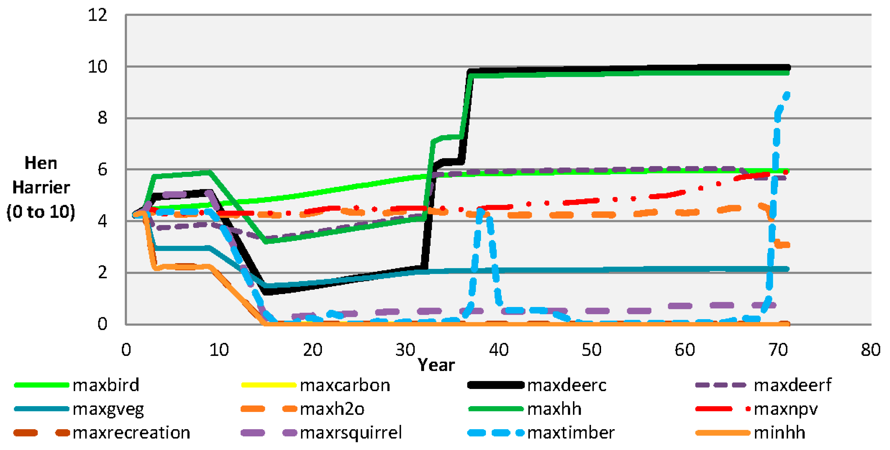
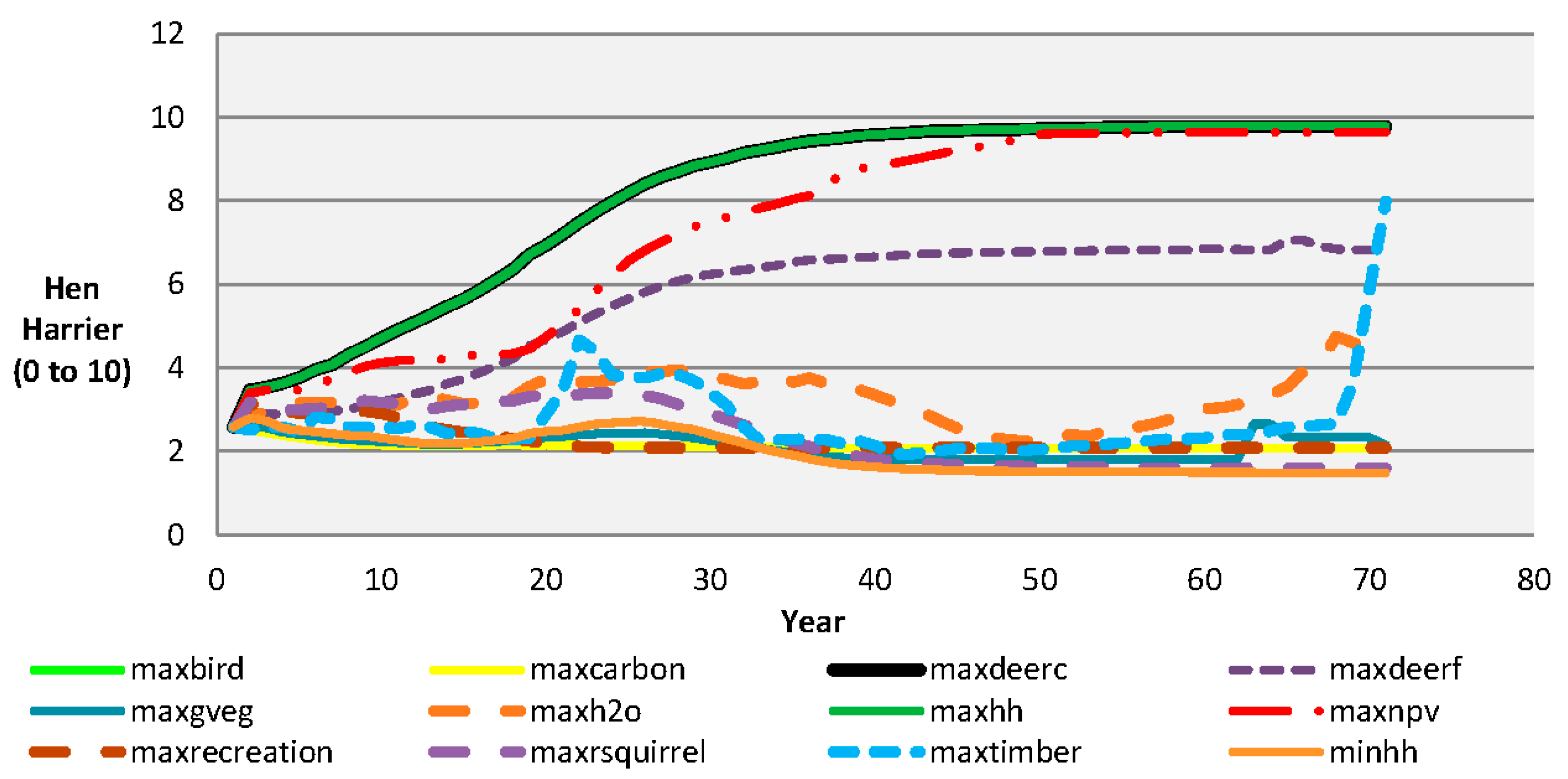
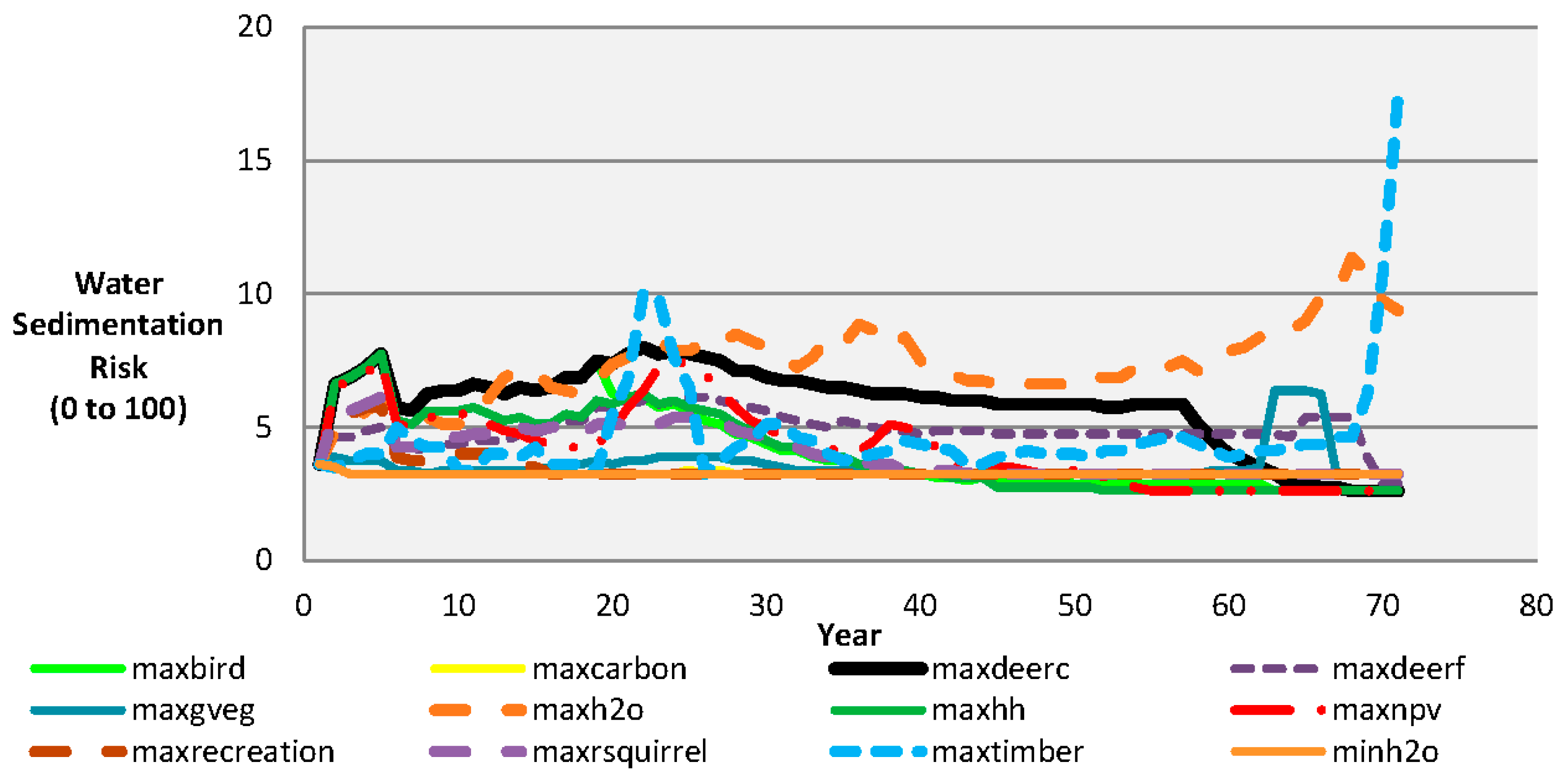
3.2. Ecosystem Services Trends Throughout the Planning Period

The type of land-use that is typically chosen when optimising each ES is presented in this section. From this point on, the presented results include land that is forest and agriculture. Each CSA will be reported on separately rather than comparatively. If a maximisation ES is presented in this section, the minimising scenario will also be presented in the same figure and vice versa.

In the maxcarbon, maxgveg and maxrec scenarios, forest stands are retained past economic or silvicultural maturity. Although these retained stands enhance multiple ES provisions, they are not suited to providing hen harrier habitat (Figure 3). Optimisation of red squirrel habitat favours mature stands; however, it does not favour the forest species currently present in either CSA. Therefore, alternative forest species are chosen to develop optimal red squirrel landscape habitability. This is illustrated in Figure 4, where the hen harrier habitat, as a result of the establishment of Scots pine stands (through afforestation and reforestation) in the maxrsquirrel scenario, is provided at a moderate level for the first 25 years. When the Scots pine stands mature, they become unsuitable for the hen harrier.

In the maxtimber scenario, many stands are allowed to reach commercial maturity; in addition, all agricultural land and all clearfelled sites are forested with timber species that can produce volume most quickly, and the model chooses a commercial rotation-based system. Large clearfelling events are scheduled during the middle of the planning period in this scenario, increasing hen harrier habitat (Figure 3 and Figure 4) but also water sedimentation risk (Figure 5). Forests are then restocked and allowed to mature in order to optimise timber production through a large clearfelling event in the final year of the planning period.

The maxbird, maxdeerc, maxnpv and maxdeerf ESs have a similar provision level of hen harrier habitat as the maxhh scenario, by providing habitat through the clearance of forest (Figure 4). The maxnpv scenario provides benefits to hen harrier habitat though clearfelling and foregoing reforestation. Deer foraging is provided by cleared forest, but more so by mature forest, while scores are particularly low for maturing forest. Therefore, in the maxdeerf scenario the model chooses younger forest stands to be clearfelled at the earliest allowable stage, while stands that are mature enough to benefit from the high ratings from the start of the planning period are retained.

In the NM CSA some agricultural land-uses have higher ES provision levels than any forest land-use. In the maxdeerf and maxbird scenarios, grassland is retained. The model chooses the higher habitat scores of forested land over some tillage land-uses for these scenarios (Figure 3). Intensive grassland-based agriculture is afforested at the beginning of the maxhh and maxdeerc scenarios in the NM CSA, which is reflected in an increase in hen harrier habitat. This hen harrier habitat provision gradually declines as these afforested stands (year 10 to 15 in Figure 3) mature. They are clearfelled as soon as they become eligible (period 30 to 35 in Figure 3). These stands are not reforested and provide very high hen harrier habitat scores associated with scrubland for the remainder of the planning period, i.e., afforestation is necessary as scrubland cannot be created straight from agricultural land.

3.3. Comparing the Trade-Offs between ESs

The intention in this section is to provide a representation of the ES provisions over the entire planning period. ES provisions can vary year to year and therefore the average level of each ES over the entire 70-year planning period is used. For each ES that is optimised, the average ES provision for that ES is improved compared to the 2012 score (

Table 5. Comparing the average ecosystem service scores with the initial 2012 ecosystem service scores. Note the Newmarket case study area includes agricultural land from this point on in the study and, as a result, the ecosystem service provisions from the two case study areas are not comparable.

	Newmarket		Western Peatland
Ecosystem service	2012	Average score	2012	Average score
Deer cover (1–10)	1.87	5.77	4.76	6.44
Deer forage (1–10)	4.91	5.57	3.21	5.39
Hen harrier (1–10)	4.25	7.14	2.59	8.09
Water sedimentation risk (0–100)	6.13	3.98	3.61	3.26
Carbon (t)	1,264,216	16,016,810	4,596,937	10,350,971
Red squirrel (1–10)	0.18	4.41	2.05	4.00
Nesting birds (1–10)	8.81	9.37	6.59	8.49
Ground vegetation (1–10)	3.60	4.86	4.26	5.54
Recreation (1-10)	2.61	6.37	3.05	5.98

). This indicates that the landscape composition in 2012 provides a mix of ESs rather than specifically targeting one individual ES. Furthermore, when comparing the average ES provision in each biophysical scenario with the corresponding 2012 level, it is clear that each CSA can facilitate increased provisions of all ESs included in this study.

The optimisation scenarios and the resulting trade-offs between all ESs for both CSAs are presented in

Table 6. The trade-offs between ecosystem servicess when optimising each ecosystem service separately (minimising for water sedimenation risk and maximising for all others).

	ES Level in More Desirable 50% of Biophysical Range
ES Optimised	Bird	Carbon	deerc	deerf	gveg	h2o	hh	NPV	Recreation	Rsquirrel	Timber	Total (WP, NM)
bird			X	X		1	X	X				4, 5
carbon					2				X	1	X	3, 3
deerc	2			2			X	2		1	1	4, 3
deerf	X	2	X		2	1	X	X	2			7, 5
gveg		X		2			1		X	X	X	5, 5
h2o	2	2	2	X			X	X	X	2	X	9, 5
hh	X		X	X		1		X				4, 5
NPV	X		2	1		X	2			2	2	6, 3
recreation		X			X					2	2	4, 2
rsquirrel		X			2				2			3, 1
timber						2		2				2, 1

Any value in a cell represents the ecosystem services whose average provision is within the more desirable 50% of the ES’s biophysical range. A “1” and “2” indicate that an ecosystem services is in the desired range for Western Peatland and Newmarket, respectively, and an “X” indicates that this is the case for both case study areas. The total number of ecosystem services in the desirable range is also presented.

. This table depicts those ESs that have an average provision level within the more desirable half of the average biophysical range (i.e., within the more desirable half of the average maximum and minimum biophysical scenario results) when optimising each ES. For all scenarios, at least one ES provision level is outside of its desired range. This indicates that a reduction in some ES provision level is always the consequence of optimising other ESs. The number of ESs that remain within their desired range is reduced particularly when an ES requires unique habitat. The optimal type of habitat for red squirrel is mature Scots pine, which, in 2012 is a minor species in both CSAs. When Scots pine is planted for the maxrsquirrel scenario, the resulting provision levels for many of the other ESs provisions decline into the less desired range. This is also typically the case for timber production, carbon sequestration and recreation provision, i.e., a total of 6 or less ES provisions are in their desired range for both CSAs as a result of optimising these ESs. In the minh2o scenario, all agricultural land is afforested during the planning period and this makes more ESs less compatible than in the WP CSA, where all land is already forested at the beginning of the planning period. The young forests in NM are less suited to providing a broad mix of ESs. When the compatibility is assessed in the WP, recreation was found to be compatible with timber production. This is unexpected, as recreation requires mature forest while timber is produced when mature forests are harvested. At the beginning of the planning period, much of the WP CSA has mature forests, i.e., a higher recreation score than the afforested areas at the beginning of the planning period in NM. Recreation and timber production is therefore more compatible when scores are averaged over the course of the planning period in the WPs. Even though, for both CSAs, there is a large clearfell in the final year of the planning period resulting in a very low recreation ES score in the final year.

4. Discussion

The concepts of integrated forest, landscape and ES management are very new in Ireland and this study has introduced these concepts to a wide range of managers and stakeholders. The model described in this study is a first attempt to quantify a wide range of ESs simultaneously, based on Ireland’s current climate and silvicultural systems. Up to now, research was done separately for different land-uses and no unified ES quantification system was available. The ES scales and scores developed in this study were produced within the academic domain, but it is expected that the model will be used in practical and operational settings in the coming years. Further development and refinement of the ES scales used in this study will benefit the approach and improve the current methods used to determine ES scales and scores.

The academic and industry stakeholders consulted at the local and national level have extensive knowledge of individual ESs quantified and of the CSAs investigated in this study. Based on the success of this study, the model will be used in a new international research project that involves many of the same stakeholders. In addition, Coillte, who also use Remsoft, is interested in incorporating several ESs into its management planning procedures.

It is important to note that the Irish model and outputs described in [49] are different from those presented in this manuscript. The Irish model in [49] involves a goal programming approach that incorporates constraints to reflect Irish forest policy and regulations and that aims to optimise stakeholder selected ecosystem provision levels. The model described in this manuscript is a more fundamental and pure biophysical model that is used to establish the absolute boundaries on the ecosystem service levels that the landscape can provide. These boundaries are then used as goals for the ecosystem services in the models used in [49].

Caveats

The following caveats to the method described should be noted:

Spatial adjacency: The model developed in this study omits spatial adjacency constraints from within the optimisation algorithm. Without spatial adjacency, some polygons (or groups of polygons) may be too small/large, or too fragmented/homogenous, thus rendering the non-spatial solutions sub-optimal [50].

Fluctuations in ES provision levels: The scenarios produce the highest and lowest cumulative scores for each ES provision over 70 years. Within these cumulative scores, considerable fluctuations happen in the annual provision levels over the planning period. This may mean that optimal solutions may not necessarily sustain the populations living within these landscapes for the entire planning period.

Landscape heterogeneity: The methods used to quantify the ES scales and scores developed in this model were chosen because they were applicable to Ireland’s landscape heterogeneity, climate and silvicultural systems. Much of the research used was based on data collected in the United Kingdom, (i.e., timber, carbon and some biodiversity) but also information from Sweden (i.e., water sedimentation risk). The ES scores used have been accepted by academic and industry experts, however the changes in heterogeneity that do happen may mean changes in the ES scores from those currently used.

Other forestry-related ESs: The ESs chosen for inclusion in this study were considered the most relevant to Irish forest policy development and forest management planning. There are of course other ESs that are influenced by forest management e.g., climate regulation, cultural heritage and identity and genepool protection. Their inclusion will be considered in future model development [12].

ESs not specific to forestry: In the NM CSA, agricultural land-uses were included in the model. However, several ESs whose provision levels are typically higher in agriculture than in forestry were not taken into account. Some examples of these include pollination, food production and the provision of fibre, fuel and other raw materials (other than wood) [12].

5. Conclusions

The results of this study show that in both CSAs there were ESs that were compatible with many others, while optimising some ESs resulted in large trade-offs with others. This result is consistent with studies in other geographical areas, which also investigated the simultaneous provision of ESs [3,51]. This study was carried out to determine the production frontier for each ES and the trade-offs with other ESs required to reach these provision levels. These biophysical ranges can assist in demonstrating to stakeholders the trade-offs and synergies that optimising one ES has on the other ESs quantified within a model. Such quantitative analysis capability will be useful when facilitating stakeholder-based management planning discussions. When combined with forest policy, land-owner behaviour and stakeholders’ preferred ES provision levels, the findings of such stakeholder discussions will be beneficial towards developing landscape level integrated management and land-use plans.

References

1. Forest Service. National Forest Inventory—Epublic of Ireland—Results; Forest Service: Wexford, Ireland, 2013. [Google Scholar]
2. Barrett, F.; Somers, M.J.; Nieuwenhuis, M. Practisfm—An Operational Multi-Resource Inventory Protocol for Sustainable Forest Management; CABI: Wallingford, UK, 2007; pp. 224–237. [Google Scholar]
3. Nieuwenhuis, M.; Tiernan, D. The impact of the introduction of sustainable forest management objectives on the optimisation of PC-based forest-level harvest schedules. For. Policy Econ. 2005, 7, 689–701. [Google Scholar] [CrossRef]
4. Turner, B.J.; Chikumbo, O.; Davey, S.M. Optimisation modelling of sustainable forest management at the regional level: An australian example. Ecol. Model. 2002, 153, 157–179. [Google Scholar] [CrossRef]
5. Alcamo, J.; Bennett, E.M. Ecosystems and Human Well-Being: A Framework for Assessment; Island Press: New York, NY, USA, 2003. [Google Scholar]
6. Gómez-Baggethun, E.; de Groot, R.; Lomas, P.L.; Montes, C. The history of ecosystem services in economic theory and practice: From early notions to markets and payment schemes. Ecol. Econ. 2010, 69, 1209–1218. [Google Scholar] [CrossRef]
7. King, R.T. Wildlife and management. N. Y. Stake Conserv. 1966, 20, 8–11. [Google Scholar]
8. Westman, W.E. How much are nature’s services worth? Science 1977, 197, 960–964. [Google Scholar] [CrossRef] [PubMed]
9. MEA. Millennium Ecosystem Assessment. Available online: http://www.unep.org/maweb/en/index.aspx (accessed on 5 Octorber 2015).
10. Costanza, R.; d’Arge, R.; de Groot, R.; Farber, S.; Grasso, M.; Hannon, B.; Limburg, K.; Naeem, S.; O’Neill, R.V.; Paruelo, J.; et al. The value of the world’s ecosystem services and natural capital. Nature 1997, 387, 253–260. [Google Scholar] [CrossRef]
11. Raudsepp-Hearne, C.; Peterson, G.D.; Bennett, E.M. Ecosystem service bundles for analyzing tradeoffs in diverse landscapes. Proc. Natl. Acad. Sci. USA 2010, 107, 5242–5247. [Google Scholar] [CrossRef] [PubMed]
12. De Groot, R.S.; Alkemade, R.; Braat, L.; Hein, L.; Willemen, L. Challenges in integrating the concept of ecosystem services and values in landscape planning, management and decision making. Ecol. Complex. 2010, 7, 260–272. [Google Scholar] [CrossRef]
13. Fléchard, M.-C.; Carroll, M.S.; Cohn, P.J.; Ní Dhubháin, Á. The changing relationships between forestry and the local community in rural northwestern Ireland. Can. J. For. Res. 2007, 37, 1999–2009. [Google Scholar] [CrossRef]
14. Tiernan, D. Redesigning Afforested Western Peatlands in Ireland: (published in): After Wise Use—the Future of Peatlands; Irish Peatland Society: Jyväskylä, Finland, 2008. [Google Scholar]
15. Cregan, M.; Murphy, W. A Review of Forest Recreation Research Needs in Ireland; COFORD: Dublin, Ireland, 2006. [Google Scholar]
16. Ní Dhubháin, Á.; Fléchard, M.-C.; Moloney, R.; O’Connor, D. Stakeholders’ perceptions of forestry in rural areas—Two case studies in ireland. Land Use Policy 2009, 26, 695–703. [Google Scholar] [CrossRef]
17. Nieuwenhuis, M.; Williamson, G.P. Harvesting coillte’s forests: The right tree at the right time. Irish For. 1993, 50, 122–133. [Google Scholar]
18. McDonagh, M. (Resource Planning Team Leader Coillte); Corrigan, E. (Ph.D candidate, University College Dublin). Personal Communication, 2012.
19. Forest Service. Irish National Forest Standard; Magner Communications: Dublin, Ireland, 2000. [Google Scholar]
20. Walters, K.R. Design and development of a generalised forest management system: Woodstock. In Proceedings of the International Symposium on Systems Analysis and Management Decisions in Forestry, Valdivia, Chile, 9–12 March 1993; Remsoft Inc.: Valdivia, Chile, 1993. [Google Scholar]
21. Farrelly, N.; Ní Dhubháin, Á.; Nieuwenhuis, M. Site index of sitka spruce (Picea sitchensis) in relation to different measures of site quality in Ireland. Can. J. For. Res. 2011, 41, 265–278. [Google Scholar] [CrossRef]
22. Horgan, T.; Keane, M.; McCarthy, R.; Lally, M.; Thompson, D. A Guide to Forest Tree Species Selection and Silviculture in Ireland; COFORD: Dublin, Ireland, 2003. [Google Scholar]
23. Forest Service. Native Woodland Scheme—Establishment; Department of Agriculture Fisheries and Food, Johnstown Castle Estate: Wexford, Ireland, 2011. [Google Scholar]
24. BFC. Yield Models for Forest Management; Forestry Commission: Alice Holt Lodge, UK, 1973. [Google Scholar]
25. Matthews, R.W.; Mackie, E.D. Forest Mensuration: A Handbook for Practitioners, 2nd ed.; Forestry Commission: Edinburgh, Ireland, 2006; p. 330. [Google Scholar]
26. Wilson, M.; Gittings, T.; O’Halloran, J.; Kelly, T.; Pithon, J. The Distribution of Hen Harriers in Ireland in Relation to Land-Use Cover, Particularly Forest Cover; COFORD: Dublin, Ireland, 2006. [Google Scholar]
27. Wilson, M.; Irwin, S.; O’Donoghue, B.; Kelly, T.; O’Halloran, J. The Use of Forested Landscapes by Hen Harriers in Ireland; COFORD: Dublin, Ireland, 2010. [Google Scholar]
28. Forest Service. Forest Service Appropriate Assessment Procedure—Appendix B Appropriate Assessment Procedure (AAP) Requirements Regarding Hen Harrier Spas and Afforestation; Forest Service: Wexford, Ireland, 2012. [Google Scholar]
29. Fennessy, J. The Collection Storage, Treatment and Handling of Broadleaved Tree Seed; COFORD: Dublin, Ireland, 2002. [Google Scholar]
30. Fennessy, J. The Collection, Storage, Treatment and Handling of Conifer Tree Seed; COFORD: Dublin, Ireland, 2002. [Google Scholar]
31. Bryce, J.M.; Macdonald, D.W. Projected changes in red squirrel habitats in craigvinean forest. Scott. For. 2000, 54, 87–90. [Google Scholar]
32. Flaherty, S.; Patenatue, G.; Close, A.; Lurz, P.W.W. The impact of forest stand structure on red squirrel habitat use. Forestry 2012, 85, 437–444. [Google Scholar] [CrossRef]
33. Waters, C.; Lawton, C. Red squirrel translocation in Ireland. In Irish Wildlife Manuals; Marnell, F., Kingston, N., Eds.; National Parks and Wildlife Service: Dublin, Ireland, 2011. [Google Scholar]
34. Mysterud, A.; Østbye, E. Cover as a habitat element for temperate ungulates: Effects on habitat selection and demography. Wildl. Soc. Bull. 1999, 27, 385–394. [Google Scholar]
35. Rodgers, M.; O’Connor, M.; Connie, O.D.; Asam, Z.-U.-Z.; Muller, M.; Xiao, L. Phosphorus Release from Forest Harvesting on an Upland Blanket Peat; COFORD: Dublin, Ireland, 2012; p. 8. [Google Scholar]
36. Eriksson, L.O.; Löfgren, S.; Öhman, K. Implications for forest management of the eu water framework directive's stream water quality requirements—A modeling approach. For. Policy Econ. 2011, 13, 284–291. [Google Scholar] [CrossRef]
37. Hutton, S.A.; Harrison, S.S.C.; O’Halloran, J. An Evaluation of the Role of Forests and Forest Practices in the Eutrophication and Sedimentation of Receiving Waters; University College Cork: Cork, Ireland, 2008. [Google Scholar]
38. Ryder, L.; de Eyto, E.; Gormally, M.; Sheehy Skeffington, M.; Dillane, M.; Poole, R. Riparian zone creation in established coniferous forests in Irish upland peat catchments: Physical, chemical and biological implications. Biol. Environ. Proc. R. Ir. Acad. 2011, 111, 41–60. [Google Scholar] [CrossRef]
39. Moorkens, E.A. Conservation management of the freshwater pearl mussel Margaritifera margaritifera. In Irish Wildlife Manuals; The Heritage Service: Dublin, Ireland, 1999. [Google Scholar]
40. Mitsova, H.; Mitas, L. Modeling soil detachment with RUSLE3D using GIS. Available online: http://skagit.meas.ncsu.edu/~helena/gmslab/denix/usle.html (accessed on 6 March 2016).
41. Sivertun, Å.; Prange, L. Non-point source critical area analysis in the gisselö watershed using GIS. Environ. Model. Softw. 2003, 18, 887–898. [Google Scholar] [CrossRef]
42. Edwards, D.M.; Jay, M.; Jensen, F.S.; Lucas, B.; Marzano, M.; Montagné, C.; Peace, A.; Weiss, G. Public preferences across Europe for different forest stand types as sites for recreation. Ecol. Soc. 2012. [Google Scholar] [CrossRef]
43. Duncker, P.S.; Barreiro, S.M.; Hengeveld, G.M.; Lind, T.; Mason, W.L.; Ambrozy, S.; Spiecker, H. Classification of forest management approaches: A new conceptual framework and its applicability to European forestry. Ecol. Soc. 2012. [Google Scholar] [CrossRef]
44. Levy, P.E.; Hale, S.E.; Nicoll, B.C. Biomass expansion factors and root: Shoot ratios for coniferous tree species in Great Britain. Forestry 2004, 77, 421–430. [Google Scholar] [CrossRef]
45. Teobaldelli, M.; Somogyi, Z.; Migliavacca, M.; Usoltsev, V.A. Generalized functions of biomass expansion factors for conifers and broadleaved by stand age, growing stock and site index. For. Ecol. Manag. 2009, 257, 1004–1013. [Google Scholar] [CrossRef]
46. Cairns, M.A.; Brown, S.; Helmer, E.H.; Baumgardner, G.A. Root biomass allocation in the world’s upland forests. Oecologia 1997, 111, 1–11. [Google Scholar] [CrossRef]
47. IPCC. Annex 3a.1biomass Default Tables for Section 3.2 Forest Land; IPCC: Geneva, Switzerland, 2003. [Google Scholar]
48. Smith, J.E.; Heath, L.S.; Jenkins, J.C. Forest Volumeto-Biomass Models and Estimates of Mass for Live and Standing Dead Trees of U.S. Forests; USDA: Washington, DC, USA, 2013. [Google Scholar]
49. Biber, P.; Borges, J.; Moshammer, R.; Barreiro, S.; Botequim, B.; Brodrechtová, Y.; Brukas, V.; Chirici, G.; Cordero-Debets, R.; Corrigan, E.; et al. How sensitive are ecosystem services in European forest landscapes to silvicultural treatment? Forests 2015, 6, 1666–1696. [Google Scholar] [CrossRef]
50. Baskent, E.Z.; Keles, S. Spatial forest planning: A review. Ecol. Model. 2005, 188, 145–173. [Google Scholar] [CrossRef]
51. Kline, J.D.; Mazzotta, M.J. Evaluating Tradeoffs among Ecosystem Services in the Management of Public Lands; USDA: Washington, DC, USA, 2012. [Google Scholar]
52. Forest Service. Forestry Schemes Manual; Department of Agriculture, Food and the Marine: Johnstown Castle Estate, Wexford, Ireland, 2011. [Google Scholar]
53. Connolly, L.; Kinsella, A.; Quinlan, G.; Moran, B. Teagasc National Farm Survey 2007; Teagasc: Athenry, Ireland, 2008. [Google Scholar]
54. Connolly, L.; Kinsella, A.; Quinlan, G.; Moran, B. Teagasc National Farm Survey 2008; Teagasc: Athenry, Ireland, 2009. [Google Scholar]
55. Connolly, L.; Kinsella, A.; Quinlan, G.; Moran, B. Teagasc National Farm Survey 2009; Teagasc: Athenry, Ireland, 2010. [Google Scholar]
56. Hennessy, T.; Kinsella, A.; Moran, B.; Quinlan, G. Teagasc National Farm Survey 2010; Teagasc: Athenry, Ireland, 2011. [Google Scholar]
57. Hennessy, T.; Kinsella, A.; Moran, B.; Quinlan, G. Teagasc National Farm Survey 2011; Teagasc: Athenry, Ireland, 2012. [Google Scholar]
58. Smith, G.; O’Donoghue, S.; Iremonger, S.; Gittings, T.; Pithon, J.; O’Halloran, J.; Wilson, M.; O’Donnell, V.; Kelly, D.; French, L.; et al. Assessment of Biodiversity at Different Stages of the Forest Cycle; University College Cork: Cork, Ireland, 2005. [Google Scholar]
59. O’Halloran, J.; Irwin, S.; Kelly, D.; Kelly, T.; Mitchell, F.; Coote, L.; Oxbrough, A.; Wilson, M.; Martin, R.; Moore, K.; et al. Management of Biodiversity in a Range of Irish Forest Types; University College Cork: Cork, Ireland, 2011. [Google Scholar]
60. Barrett, F.; Nieuwenhuis, M.; Doyle, M. The practisfm multi-resource inventory protocol and decision support system: A model to address the private forest resource information gap in Ireland. Ir. For. 2009, 64, 5–20. [Google Scholar]
Figure 1. Location of both case study areas: Western Peatlands (top); and Newmarket (bottom).
Forests 07 00128 g001
Figure 2. The essential steps and components in the biophysical modelling process.
Forests 07 00128 g002
Figure 3. Hen harrier biophysical range and trade-off when maximising other ecosystem services over the planning period in the NewmarketM case study area. Maxcarbon, maxrecreation, follow a similar trend as minh.
Forests 07 00128 g003
Figure 4. Hen harrier biophysical range and trade-off when maximising other ESs over the planning period in the Western Peatland case study area.
Forests 07 00128 g004
Figure 5. Water sedimentation risk biophysical range and trade-off when maximising other ecosystem services over the planning period in the Western Peatland case study area. Maxcarbon and maxrecreation follow a similar trend to minh2o.
Forests 07 00128 g005