Article

How Do Urban Forests Compare? Tree Diversity in Urban and Periurban Forests of the Southeastern US

1
Department of Biological Sciences, The University of Alabama, Tuscaloosa, AL 35401, USA
2
Faculty of Natural Sciences and Mathematics, Biology Program, Universidad del Rosario, Bogotá D.C., Colombia
3
School of Forestry and Wildlife Sciences, Auburn University, Auburn, AL 36849, USA
*
Author to whom correspondence should be addressed.
Forests 2016, 7(6), 120; https://doi.org/10.3390/f7060120
Submission received: 29 April 2016 / Revised: 31 May 2016 / Accepted: 3 June 2016 / Published: 9 June 2016
(This article belongs to the Special Issue Urban and Periurban Forest Diversity and Ecosystem Services)

Abstract

:
There is a need to understand how anthropogenic influences affect urban and periurban forest diversity at the regional scale. This study aims to compare urban and periurban tree composition along a geographic gradient, and test hypotheses about species composition and ecological homogeneity. We paired urban forest (UF) data from eight cities across the southeastern US with periurban forest (PF) data from the USDA Forest Service Forest Inventory and Analysis program. We found that tree diversity, as well as both observed and estimated species richness values were greater in UF versus PF. Community size structure analysis also indicated a greater proportion of large trees and greater numbers of non-native, invasive, and unclassified tree species in the UF versus the PF, regardless of location. Both forest type and ecological province had a significant effect on community species composition, with forests closer together in space being more similar to each other than those more distant. While land use change and management has been associated with ecological homogenization in human dominated landscapes, we found that species composition was more dissimilar along latitudinal lines than compared to between forest types, refuting this hypothesis, at least in terms of tree diversity.

Graphical Abstract

1. Introduction

Rapid urbanization and land use change in proximity to urban areas has led to the alteration of structure and composition of forests [1]. Novel ecosystem assemblages have developed in both urban and periurban forests in response to land use change, as well as species introductions, ecological disturbance, and sociopolitical and economic shifts [2,3,4,5]. As natural landscapes are altered by urbanization, there is a gap in our understanding of the implications these changes might have on regional urban and periurban tree diversity. For example, have anthropogenic influences resulted in a homogenization of species composition within urban forests across regional scales? Are human-dominated landscapes providing adequate areas for native tree species? Is the species composition of urban areas more or less resistant to climate change, as compared to adjacent periurban forests?
There is mounting evidence suggesting that more diverse ecosystems have increased resistance to pests and disease [5,6,7,8]. Urban forests with low tree diversity may be at substantial risk in terms of potential alteration from ecological disturbances. For example, Dutch elm disease caused the mortality of millions of elm trees [5], greatly changing the urban forest composition and structure in cities such as Boulder City, NV and Chicago, IL in the United States (US) [9,10]. Since then, urban forester managers and planners have placed a higher value on urban tree diversity to limit future disturbances [11].
Because tree diversity is associated with enhanced ecosystem resistance to disturbances, tree diversity can also potentially increase resistance and adaptation to the impacts of a changing climate [8]. More diverse populations have greater adaptive capacity and thus are able to better withstand changes in ambient biophysical conditions [12,13]. Climate change has already caused shifts in tree species ranges and phenology [14,15]; if changes continue as predicted, this may lead to future unsuitability of species in both urban and periurban forests.
Invasive woody plants have had well-documented negative effects on both urban and periurban landscapes [16,17,18]. The presence of invasive plant species has been associated with reduced biodiversity and increased biotic homogenization [4,16], changes in forest structure, altered natural disturbance regimes [19,20], and subsequently modified ecosystem processes [21,22]. Moreover, innocuous non-native species may become invasive; worldwide, an estimated 62% of invasive species were introduced for horticulture and 13% for forestry [4]. For example, Pyrus calleryana Decne. has escaped cultivation in many areas of the US as a result of hybridization, forming dense homogenous plant communities and outcompeting local species [23,24]. Pinus pinaster Aiton and P. halepensis Mill. have negatively impacted water resources and biodiversity, as well as increased fire severity in Cape Town, South Africa [17]. Additionally, with changing climate, species that have not yet previously posed an invasive threat may become so with range shifts into areas more suitable for the non-native species [25].
Because non-native tree species (e.g., P. calleryana and Acer platanoides L. in the US) often have a broader niche that allows them to thrive in urban locales, these species have been historically planted intentionally throughout different regions of the world. These human planting preferences have led to the hypothesis that human dominated landscapes are undergoing ecological homogenization [3]. However, few studies have quantified similarities in tree species composition across urban and rural or periurban forest gradients.
Given this lack of information, our study aims to characterize community structure and composition of urban forests in the southeastern United States (SE US), and compare these metrics against adjacent periurban forests. For this study, we defined urban forests (UF) as a collection of trees within urban boundaries and its mixed land uses as well as in privately and publicly owned properties [26]. UF therefore included high- and low-density residential areas, as well as commercial, institutional, and industrial land uses. Periurban forests (PF) were defined as non-urban, forested areas located within 25 km of an urban city center. The SE US is an ideal location for this type of study due to its recognition as a tree diversity hotspot within North America and classification as a priority ecoregion for conservation [27,28]. We hypothesize that greater tree diversity exists in UF, with a greater number of both non-native and native species [29]. Additionally, a greater prevalence of human disturbance (as is the case in urban areas versus periurban areas) will result in a greater number of unintentional introductions, resulting in a prevalence of non-native and invasive species in UF versus PF [4]. We also expect that trees in UF will be smaller than those in adjacent PF. Moreover, we hypothesize that the species community composition among the UF of the different localities sampled will be more closely linked to geography than forest type (UF vs. PF).

2. Materials and Methods

2.1. Data Acquisition

Urban forest data were collected by independent research groups in eight localities (Figure 1; Table 1) between 2008 and 2014. The data were compiled into the Southeastern Urban Tree Database as part of a collaborative project sponsored by several universities and the Southern Research Station of the US Department of Agriculture (USDA) Forest Service. All UF data were collected using, or based on, the i-Tree Eco protocol [30], a standard sampling and inventory protocol that has been used extensively for sampling urban forests throughout the world [31,32]. In Gainesville, FL, plots were established randomly across varied urban land uses, such as commercial, vacant, and residential [33]. (See [22,30,31,32,33,34,35,36] for specific information regarding land use definition and the percentage of these in the different localities.) Four Virginia locations (Charlottesville, Abingdon, Winchester, and Roanoke City; [36]), as well as east Orlando, Florida were sampled using stratified random sampling, stratifying by land use [22]. One location in Virginia (Falls Church) was sampled using a randomized grid. Plots were selected in the City of Atlanta (Fulton and DeKalb counties) as part of a sub-study of the Proctor Creek Watershed (a Federal Urban Waters Project, [37]). Plots were selected via random generation of GIS locations from three land use class strata (residential, transportation, and all other) in proportion to US Geographical Survey land use land cover classifications. All urban localities in the study area were sampled using randomly selected 0.04 ha plots established within city limit boundaries (with the exception of east Orlando, where plots were placed within a 200 km2 area around an eddy flux tower).
Each tree or palm with diameter at breast height (DBH; measured at 1.37 m from the ground) greater than 2.5 cm was measured and its species name recorded. Other measurements included height, land use, crown width, and crown light exposure. If a tree had multiple stems below DBH, it was counted as a singular tree, and the largest diameters (up to six) were recorded. For specific measurement methods, refer to [22,30,33,34,35,36]. For multi-stemmed trees, we calculated the quadratic mean diameter to represent the DBH underlying a tree with the same total tree cross-sectional area.
All periurban data were from forested areas sampled with the USDA Forest Inventory and Analysis (FIA) protocol which were located within 25 km of an urban city center. Data were obtained from the USDA Forest Service datamart [40]. FIA data encompass areas that range from suburban to rural [2], but include only “forest land”, which is defined as having an area of at least 0.4 ha with at least 10% canopy cover of live tree species of any size, either at the time of sampling or in the past, where the land is not subject to non-forest use which would prevent normal tree regeneration and succession (e.g., regular mowing, or grazing) [28]. All FIA plots are measured on a cyclic basis throughout the United States by the USDA Forest Service, with the intention of collecting data on an estimated 1 in 2428 hectares of land in the country to monitor the forest resources of the US. We extracted FIA data within a radius of 25 km around each urban forest location using ArcMap 10.1. The FIA plot locations are “fuzzed” and do not report exact spatial coordinates to comply with privacy issues; thus locations are between 0.8 and 1.6 km of the actual plot. Accordingly, we analyzed results on a community scale rather than by plot [41,42], so we estimated location error to be small. We obtained data from the years 2010–2013 for Virginia, and 2009–2013 for Georgia and Florida to obtain the maximum number of tree measurements while excluding re-measured trees. In three instances, data were also extracted from surrounding states because the 25 km buffer extended past state lines (Figure 1). Years extracted in those states were between 2009 and 2013, excluding 2009 if a re-measurement occurred in 2013.
The FIA plots consist of groups of four subplots that cover an area of approximately 0.067 hectares, with a microplot approximately 0.001 hectares in area located within each subplot. Woody plants with DBH values less than 12.7 cm but greater than or equal to 2.54 cm are measured only in the microplots. We used an expansion factor of 12.46 for the tree counts within microplots to adjust for their smaller sample plot. Tree data collected includes condition, species, DBH, height, and location within plot (for more information on FIA data collection, see [43]). In contrast to the i-Tree protocol, under the FIA protocol a tree that splits below DBH is recorded as more than one tree. Since trees that split between 0.3 m and 1.37 m are given the same cardinal distance and direction, we were able to combine multiple stems using the quadratic mean diameter to match the two protocols in these cases. We could not, however, differentiate between trees that split less than 0.3 meters from the ground and those which had not been split. Thus, we performed analyses with measures of stem density, as well as with basal area to account for this potential error.

2.2. Statistical Analyses

Unless otherwise stated, statistical analyses were carried out in R version 2.2-1 [44] with the vegan package [45]. We characterized species richness for each location using a bootstrap method to estimate the expected number of species in an area, using rare species to quantify how many species were likely unobserved. Species accumulation curves were created by graphing the area sampled rather than by the number of plots to account for different plot sizes. Curves were visually analyzed to verify species richness to avoid confounding results from locations with differing sampling intensities and plot sizes. Diversity by location was quantified using both the Shannon-Weaver (H′) and the Inverse Simpson’s (λ−1) Indices:
H = p i   ln p i
λ 1 = ( p i 2 ) λ 1
where: pi is the proportion of individuals in the ith species for a particular location. We did not quantify plot-level diversity because of differences in data collection methods between urban and periurban plots, such as different plot sizes and shapes. Additionally, PF plots contained, on average, many more trees than UF plots because all plots were classified as “forest land.” Diversity metrics (species richness, Shannon-Weaver, and Inverse Simpson’s) were analyzed with all species, as well as with only native and naturalized species to answer questions about species which could be expected to persist without further human influence. We defined “naturalized” species as those which are invasive or have been recorded as invasive anywhere within the US [46].
To assess community structure, we used graphical as well as statistical means. We focused on DBH-based measures of structure rather than other measures (e.g., tree height or biomass) due to the strong correlation between DBH and both biomass and tree height, and the lack of local and UF-specific biomass equations for most UF species. We first analyzed DBH distributions graphically according to forest type and location, and investigated significant differences between PF and UF as well as among locations using the Log-Rank and Wilcoxon tests via the SAS (9.3) procedure PROC LIFETEST [47].
Species composition was investigated by categorizing tree species into native, non-native, invasive, and unclassified. Native status was defined by classification in i-Tree [48], supplemented by the USDA PLANTS database [49]. Invasive species classification was defined using invasive plant species lists by state [50,51,52]. Species with any level of invasive status (e.g., threat level categorizations) within the state in which they were sampled were considered to be invasive. Trees were unclassified if they were either measured only to the genus-level or were cultivars with unspecified origin. To further understand community similarities or dissimilarities, we used a permutational ANOVA (PERMANOVA) [45] to determine whether differences in community structure were due to urbanization, geographic area, or both [53,54]. We included ecological province and land use (urban vs. periurban) in the model and used 999 permutations, following Anderson and Walsh [50]. Community differences were quantified using the Raup-Crick metric, which measures the similarities or dissimilarities between communities [55,56]. The Raup-Crick metric allows for comparisons between communities with varied numbers of species and sampling sizes, whereas other common similarity metrics such as Jaccard’s could be skewed due to dissimilarities in species richness [55,56,57]. Using a matrix of comparisons between all pairs of associations, the Raup-Crick index compares observed number of species with the distribution of co-occurrences generated from 200 Monte Carlo random replicates [55]. The computed index ranges from a value of 1.0 indicating no similarity, to 0 indicating identical similarity. To further visualize the results, we created a dendrogram from a Raup-Crick dissimilarity metric to compare each site [55], utilizing presence/absence data to prevent bias from the differences in plot sizes between UF and PF samples.

3. Results

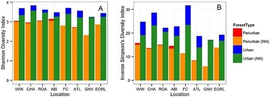
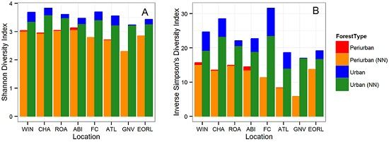
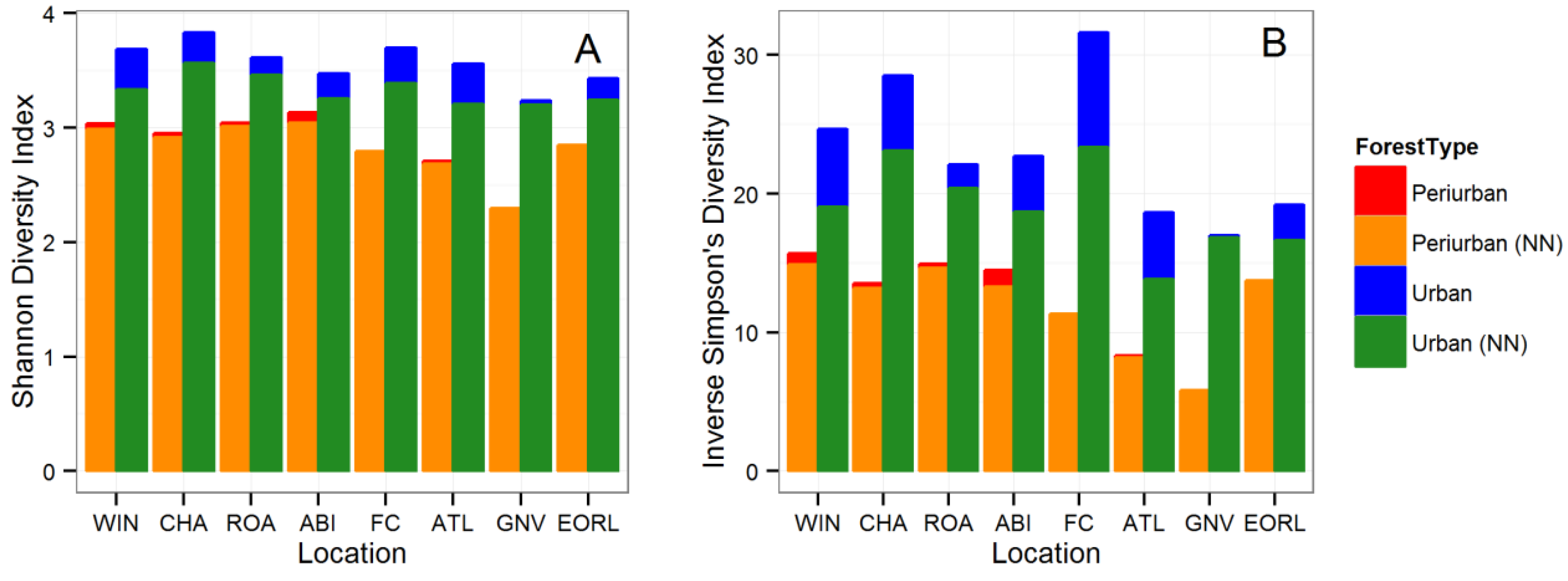
3.1. Tree Diversity Comparisons

In all localities except for Abingdon, VA, species richness values (both observed and estimated) were greater in UFs (Figure 2). The range of estimated number of species per location was 63–124 in UFs versus 35–64 in the PFs. Abingdon had the greatest number of species in its PF and the least number of species in its UF; however, species richness was not significantly different between its PF and UF (63.6 ± 2.5 and 63.2 ± 3.5, respectively; Figure 2). Roanoke’s UF had the greatest number of species overall (124 and 106; estimated and observed), while East Orlando’s PF had the fewest number of species (35 and 30; estimated and observed). In six of the eight locations, species richness, as illustrated by species accumulation curves (Figure 3 and Figure S1), was clearly greater in the UF. Differences were more difficult to distinguish between the PF and UF of Abingdon and Atlanta due to discrepancies in sample size.
Tree diversity as described with both the Shannon and Inverse Simpson’s indices was greater in UF (Figure 4). These indices indicate that the most diverse PFs were less diverse than the least diverse UFs regardless if analyses were based on biomass or stem counts. Gainesville (both PF and UF) had the lowest diversity with both indices (2.3 and 3.2, for Shannon; 5.8 and 17.0 for Inverse Simpson’s, for PF and UF, respectively), when compared to other UF and PF. As measured by the Shannon Index, Charlottesville’s UF had the greatest diversity; as measured by the Inverse Simpson’s Index, and Falls Church’s UF has the highest diversity. Overall, the PF had greater relative abundance of the most common species than the UF (PF ranged from 15% to 36%, whereas UF ranged from 7% to 15%). This measure serves as an indicator of diversity as it is significantly related to the Shannon Diversity Index, with lower relative abundance of the most common species attributed to greater diversity [11]. Gainesville’s PF had the greatest relative abundance of the most common species (36%, Pinus elliottii Engelm.).

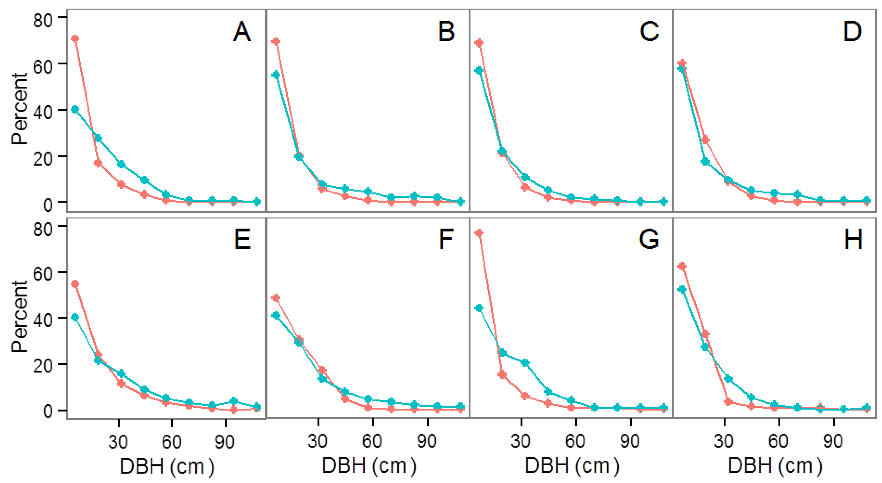
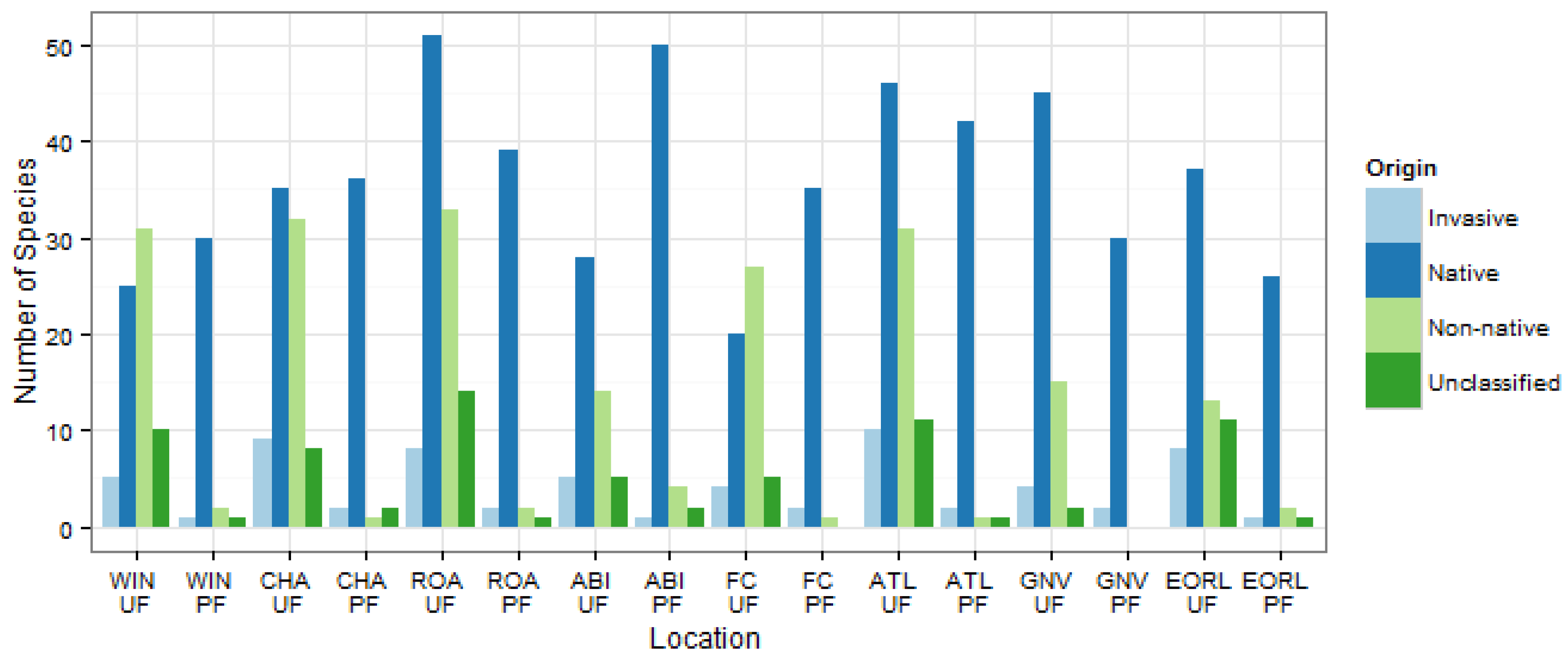
3.2. Community Structure and Composition

The UFs and PFs presented mixed results in regards to community structure and composition. Community size structure was similar regardless of location or forest type. All locations had reverse J distributions (Figure 5), with a larger presence of small trees and fewer large trees. A significantly greater proportion of trees from PF had smaller diameters than trees from UF (Wilcoxon p < 0.0001). UF had a greater proportion of large (<100 cm) trees, though this difference was not significant, indeed, only three of eight PFs had trees in that size category (Log-Rank p = 0.1057).
Altogether, there were 181 species that were present in UF but absent in PF, and 23 that were present in PF but absent in UF. The most widespread species was Acer rubrum L., which was present in every site (regardless of PF or UF location) and was within the three most common species for five of the eight PF locations and one of the eight UF locations (Table S1). Other widespread species include Carya glabra (Mill.) Sweet (present in all PF and six of the eight UF) and Prunus serotina Ehrh. (present in seven of the eight PF and UF). There were many species which were widespread in UF but absent in PF, such as Lagerstroemia indica L. and P. calleryana. Both were recorded in seven of the eight UF but not in any PF. The UF and PF had similar proportions of palms, with 1.0% in the UF and 0.8% in the PF.
There were greater numbers of non-native, invasive, and unclassified species in the UF versus the PF, regardless of location (Figure 6). Winchester and Falls Church UF had a greater number of non-native species than native species (36 versus 25 for Winchester, and 20 versus 31 for Falls Church). There was no common pattern describing the proportion of native species by forest type. By counts of individuals, PF had a substantially greater proportion of native trees in every location (Figure S2). Fewer than 50% of the trees in the UF of Winchester were native, but all other locations had communities where at least 50% of the trees were native. There were six invasive species throughout all PFs, and every invasive species found in PF was also found in UF. There were 19 additional invasive species found across our UF sample, with 10 found in Atlanta alone. However, based on numbers of trees, the UF in Atlanta had a smaller proportion of invasive trees than that of PF (Figure S2).
There was a significant effect (PERMANOVA, p < 0.05) of both forest type (Pseudo-F(1,15) = 5.003, p = 0.001) and ecological province (Pseudo-F(2,15) = 4.845, p = 0.001) on community species composition (Table S2). The Raup-Crick metric indicated that community species composition was more dissimilar between localities in Florida and Virginia than they were between UF and PF (Figure 7). Gainesville and East Orlando, regardless of forest type, had very similar communities. In Virginia, PF communities were more similar to each other than UF communities. The more northern Virginia UF communities with lower elevation gradients (Winchester and Falls Church) were more similar to each other than they were to the more southern, more elevated Virginia communities. Atlanta’s UF was more similar to its and Virginia’s PF than to any other UF.

4. Discussion

Tree species richness and diversity was greater in UF, which was expected (Figure 2, Figure 3 and Figure 4) [29]. Moreover, in two cases (Atlanta and Abingdon), the species accumulation curves show that sampling efforts were vastly different. On the other hand, the PF curve in Atlanta, when viewed at its full extent, shows a lessened slope indicative of fewer remaining (uncounted) species (Figure S1). While it could be argued that a large urban center like that of Atlanta may require a buffer larger than our chosen distance of 25 km, this distance (although arbitrary) represented a balance to limit geoclimatic variability and link to direct urban impacts. The use of estimated numbers of species rather than actual sampled numbers of species mitigates the effects of varying sampling efforts, but does carry with it uncertainty that should be addressed in future studies.
In forested ecoregions of North America, an estimated 1/3 of urban trees are planted; the rest originate from remnant or regenerated forest [58]. Therefore, UF often contain similar forest communities to PF while also containing highly altered planted communities, making it unsurprising that species found in PF are almost all in UF. The additional species richness in UF (181 species in UF not found in PF) is no doubt due to human planting or introductions of non-native species [4] and the maintenance of otherwise unfit species through fertilization and irrigation [3]. The UF had similar numbers of native species as the PF, but proportionally many more non-native species (Figure 6). Across all locations, all but one UF (Gainesville) had proportionally more non-native species than that of the 15% reported for riparian forests in urban areas of Manaus, Brazil [59] for example, and half of our UF study sites had more than twice this proportion, supporting a hypothesis of a management effect.
In North America, 77% of invasive species introductions are a result of horticulture plantings and 14% are via forestry [4]. This unintentional introduction of invasive species was noticeable in the UF, where numbers of invasive species were greater than in PF (Figure 6). Interestingly, P. calleryana, which was found in all but one of the urban locations and has been widely planted throughout the region, is now considered to be an invasive species [11,50,51,52]. Although less than 1% of woody plant introductions become invasive, this underscores the need to monitor non-native species [4]. Likely, the greater proportion of invasive trees in Atlanta’s PF is due to the large amount of human activity within the area. Indeed, the percent of developed land was positively correlated with the number of invasive species for both the PF and UF (data not shown). Atlanta’s PF was more urbanized than the other cities in this study, with a greater proportion of its land cover area classified as developed [60]. Unsurprisingly, the two invasive species found in the PF of Atlanta (Ailanthus altissima (Mill.) Swingle and Albizia julibrissin Durazz.) commonly invade disturbed areas [61].
There is a growing body of research on the structural and ecological dynamics of UFs using permanent field plot and forest inventory methods similar to the ones presented in this study [2,3,5,22,33,35,58] (and citations therein). The field measurement protocols in these disparate studies are, however, often different because of (for example) land use definitions, the stem size criteria for differentiating tree and shrub growth forms, and the presence of multi-stemmed tall woody shrubs in certain biomes (e.g., mangroves, shrublands) [2,30,33]. However, this study´s use of the same UF and PF inventory protocols and tree size criteria eliminated many of these issues. Similarly, we found that PFs were found to have a greater proportion of smaller DBH trees when compared to UF (Figure 5). This was not surprising, considering that PFs are likely to have an understory component containing saplings, due to planting or natural regeneration. On the other hand, only UF plots falling in vacant areas, parks or remnant forest patches would be likely to have comparable understories [58]. However, we did not measure the age nor assess the origin of sampled trees in our study.
Overall, we found greater species-level homogeneity in PFs than in UFs as evidenced by a greater relative abundance of the most common species in the region’s PFs. The PF of Gainesville was especially homogenous and other PF areas with low diversity were made up of very few species; greater than 50% of the trees in the PF of Gainesville were pines (primarily Pinus taeda L. and P. elliottii). This is likely a result of human intervention and legacy effects of past land use practices favoring pine plantations [1,27,62], and also a result of the generally lower tree species richness in the naturally pine-dominated landscapes sampled in this study. While hardwood-dominated depressional wetlands of this region contain higher tree diversity, our sample included few PF forests of this type. The more northern locations (those in Virginia), with their prevalence of non-native species within their UF (Figure 6), had more distinct PF and UF communities (Figure 7). Conversely, Florida locales had fewer non-native tree species, which could explain the similarities between the PF and UF in those locations. This is reflective of the lower natural tree species diversity in pine-dominated outer coastal plain landscapes sampled in this study, versus broadleaf and mixed forests, which are dominated by hardwoods and other species [27,28].
More importantly, species composition analyses indicated that urban forests were more similar to their periurban counterparts within eco-zone than were urban forests to each other, indicating that UFs are strongly influenced by the natural diversity patterns in the local vegetation. This result refutes the hypothesis of ecological homogeneity across urban areas, at least in terms of tree diversity. If homogeneity were to hold true in this region, we would have expected the urban locations to be more similar to each other, regardless of ecoregion. Instead, there was a clear distinction due to ecoregion. The results of the PERMANOVA showed that species composition of urban forest was significantly different than periurban, and significant differences also were found among urban ecological provinces.
The increased diversity in UF was a likely result of the greater diversity of the Central Hardwood forests, as well as greater landscape heterogeneity, which has been shown to result in more diverse communities [63]. However, the PF in Abingdon had an elevation gradient of greater than 1000 meters (Table 1), which could support a larger range of plant communities [64]. Abingdon’s PF had species richness which was comparable to not only its UF, but also that of Falls Church. The smaller species richness values in Abingdon’s UF may be a result of Abingdon’s less urbanized character (with a population density of <400 people/km2) and correspondingly fewer opportunities for planted species and less heterogeneity.

5. Conclusions

Our results indicate that urban tree species distributions are not geographically homogenous throughout the SE US. Urban forests in this region have maintained a fair amount of native species, and thus are a reflection of their respective periurban tree communities. Our conclusions are, however, somewhat limited by different plot size and measurement techniques used in the urban (i-Tree) and periurban (FIA) protocols. On the other hand, with the relatively recent (2014) implementation of urban FIA sampling, there is a need to develop techniques and metrics to compare the data that are available in order to further investigate hypotheses about the impacts of urbanization on trees further into the future.
Utilizing existing SE US urban forest data collected under standardized inventory and monitoring protocols, as well as available data from the USDA Forest Service FIA program, we used a novel approach to investigate urban forest community composition relative to adjacent periurban forests along a geographic and urban to rural gradient. Comparing community composition and structure between urban forests and their periurban counterparts could be used further to better assess the ecological stability and sustainability of an area in the face of climate change and urbanization. Overall, our findings indicate that urban forests, with their great diversity, should fare well in the face of future global changes. However, care should be taken to monitor non-native and invasive species and to ensure that the species and size composition support sustainability of both urban and periurban forests. In the future, more comprehensive studies should be undertaken that include more global cities to encompass a larger variety of land uses and management histories, as well as a wider range of vegetation types, to gain a more complete understanding of regional anthropogenic influences on diversity in PFs and UFs.

Supplementary Materials

The following are available online at www.mdpi.com/1999-4907/7/6/120/s1, Table S1: Common species by location, Table S2: PERMANOVA results, Figure S1: Species accumulation curves by location, Figure S2: Origins of trees by locations.

Acknowledgments

The authors would like to thank Dudley Hartel at USDA Forest Service-Urban Forestry South for funding and direction. Funding for this project and for publishing of this manuscript was provided by a grant from the US Forest Service (Forest Service Agreement Number 13-CS-11330144-061, titled “Regional Urban Forest i-Tree Eco Inventory Study”). Data for VA studies were generously provided by Dr. P. Eric Wiseman (Virginia Tech College of Natural Resources and Environment), whose funding was provided in part by USFS UCF formula funding via VA Dept. of Forestry, and in part by USDA National Institute of Food and Agriculture McIntire-Stennis formula funding. We would also like to thank multiple municipal and county employees and students who collected data, and the Staudhammer and Starr labs for valuable feedback on earlier versions of the manuscript.

Author Contributions

C.S. and A.B conceived and designed the experiments; A.B. analyzed the data; F.E. and C.S. contributed reagents/materials/analysis tools; C.S., A.B., F.E, A.C, and G.S. wrote the paper.

Conflicts of Interest

The authors declare no conflict of interest. USDA Forest Service—Urban Forestry South was responsible for the collection of data in Atlanta, GA; however, this sponsor had no role in the design of the study; in the analyses, or interpretation of data; in the writing of the manuscript, and in the decision to publish the results.

Abbreviations

The following abbreviations are used in this manuscript:
DBHDiameter at breast height
FIAForest Inventory and Analysis
PERMANOVAPermutational Analysis of Variance
PFPeriurban forests
SE USSoutheastern United States
UFUrban forests
USUnited States
USDAUnited States Department of Agriculture

References

  1. Wear, D.N. Forecasts of Land Uses. In The Southern Forest Futures Project: Technical Report; Greis, J.G., Ed.; USDA Forest Service: Washington, DC, USA, 2013; pp. 45–72. [Google Scholar]
  2. Conway, T.M.; Bourne, K.S. A comparison of neighborhood characteristics related to canopy cover, stem density and species richness in an urban forest. Landsc. Urban Plan. 2013, 113, 10–18. [Google Scholar] [CrossRef]
  3. Groffman, P.M.; Cavender-Bares, J.; Bettez, N.D.; Grove, J.M.; Hall, S.J.; Heffernan, J.B.; Hobbie, S.E.; Larson, K.L.; Morse, J.L.; Neill, C.; et al. Ecological homogenization of urban USA. Front. Ecol. Environ. 2014, 12, 74–81. [Google Scholar] [CrossRef]
  4. Richardson, D.M.; Rejmanek, M. Trees and shrubs as invasive alien species—A global review. Divers. Distrib. 2011, 17, 788–809. [Google Scholar] [CrossRef]
  5. Raupp, M.; Cumming, A.; Raupp, E. Street Tree Diversity in Eastern North America and Its Potential for Tree Loss to Exotic Borers. Arboric. Urban For. 2006, 32, 297–304. [Google Scholar]
  6. Subburayalu, S.; Sydnor, T.D. Assessing street tree diversity in four Ohio communities using the weighted Simpson index. Landsc. Urban Plan. 2012, 106, 44–50. [Google Scholar] [CrossRef]
  7. Alvey, A.A. Promoting and preserving biodiversity in the urban forest. Urban For. Urban Green. 2006, 5, 195–201. [Google Scholar] [CrossRef]
  8. Thompson, I.; Mackey, B.; McNulty, S.; Mosseler, A. Forest Resilience, Biodiversity, and Climate Change. In A Synthesis of the Biodiversity/Resilience/Stability Relationship in Forest Ecosystems; Technical Series No. 43; Secretariat of the Convention on Biological Diversity: Montreal, Canada, 2009; p. 67. [Google Scholar]
  9. McPherson, E.; Simpson, J.R. Carbon dioxide reduction through urban forestry: Guidelines for professional and volunteer tree planters. Gen. Tech. Rep. 1999, 171, 237. [Google Scholar]
  10. Dreistadt, S.H.; Dahlsten, D.L.; Frankie, G.W. Urban Forests and Insect Ecology. Bioscience 2015, 40, 192–198. [Google Scholar] [CrossRef]
  11. Kendal, D.; Dobbs, C.; Lohr, V.I. Global patterns of diversity in the urban forest: Is there evidence to support the 10/20/30 rule? Urban For. Urban Green. 2014, 13, 411–417. [Google Scholar] [CrossRef]
  12. Chapin, F.S., III; Zavaleta, E.S.; Eviner, V.T.; Naylor, R.L.; Vitousek, P.M.; Reynolds, H.L.; Hooper, D.U.; Lavorel, S.; Sala, O.E.; Hobbie, S.E.; et al. Consequences of changing biodiversity. Nature 2000, 405, 234–242. [Google Scholar] [CrossRef] [PubMed]
  13. Cumming, G.S.; Olsson, P.; Chapin, F.S.; Holling, C.S. Resilience, experimentation, and scale mismatches in social-ecological landscapes. Landsc. Ecol. 2013, 28, 1139–1150. [Google Scholar] [CrossRef]
  14. Walther, G.-R.; Post, E.; Convey, P.; Menzel, A.; Parmesan, C.; Beebee, T.J.C.; Fromentin, J.-M.; Hoegh-Guldberg, O.; Bairlein, F. Ecological responses to recent climate change. Nature 2002, 416, 389–395. [Google Scholar] [CrossRef] [PubMed]
  15. Cleland, E.E.; Chuine, I.; Menzel, A.; Mooney, H.A.; Schwartz, M.D. Shifting plant phenology in response to global change. Trends Ecol. Evol. 2007, 22, 357–365. [Google Scholar] [CrossRef] [PubMed]
  16. Motard, E.; Muratet, A.; Clair-Maczulajtys, D.; MacHon, N. Does the invasive species Ailanthus altissima threaten floristic diversity of temperate peri-urban forests? Comptes Rendus-Biol. 2011, 334, 872–879. [Google Scholar] [CrossRef] [PubMed]
  17. Gaertner, M.; Larson, B.M.H.; Irlich, U.M.; Holmes, P.M.; Stafford, L.; van Wilgen, B.W.; Richardson, D.M. Managing invasive species in cities: A framework from Cape Town, South Africa. Landsc. Urban Plan. 2016, 151, 1–9. [Google Scholar] [CrossRef]
  18. Staudhammer, C.L.; Escobedo, F.J.; Holt, N.; Young, L.J.; Brandeis, T.J.; Zipperer, W. Predictors, spatial distribution, and occurrence of woody invasive plants in subtropical urban ecosystems. J. Environ. Manag. 2015, 155, 97–105. [Google Scholar] [CrossRef] [PubMed]
  19. Vitousek, P.; D’Antonio, C.; Loope, L.L.; Westbrooks, R. Biological invasions as global environmental change. Am. Sci. 1996, 84, 468–478. [Google Scholar]
  20. Crossman, N.D.; Bryan, B.A.; Cooke, D.A. An invasive plant and climate change threat index for weed risk management: Integrating habitat distribution pattern and dispersal process. Ecol. Indic. 2011, 11, 183–198. [Google Scholar] [CrossRef]
  21. Escobedo, F.J.; Kroeger, T.; Wagner, J.E. Urban forests and pollution mitigation: Analyzing ecosystem services and disservices. Environ. Pollut. 2011, 159, 2078–2087. [Google Scholar] [CrossRef] [PubMed]
  22. Horn, J.; Escobedo, F.J.; Hinkle, R.; Hostetler, M.; Timilsina, N. The Role of Composition, Invasives, and Maintenance Emissions on Urban Forest Carbon Stocks. Environ. Manag. 2015, 55, 431–442. [Google Scholar] [CrossRef] [PubMed]
  23. Schierenbeck, K.A.; Ellstrand, N.C. Hybridization and the evolution of invasiveness in plants and other organisms. Biol. Invasions 2009, 11, 1093–1105. [Google Scholar] [CrossRef]
  24. Vincent, M.A. On the Spread and Current Distribution of Pyrus calleryana in the United States. Castanea 2005, 70, 20–31. [Google Scholar] [CrossRef]
  25. Thuiller, W. Biodiversity: Climate change and the ecologist. Nature 2007, 448, 550–552. [Google Scholar] [CrossRef] [PubMed]
  26. Konijnendijk, C.C.; Ricard, R.M.; Kenney, A.; Randrup, T.B. Defining urban forestry—A comparative perspective of North America and Europe. Urban For. Urban Green. 2006, 4, 93–103. [Google Scholar] [CrossRef]
  27. Ricketts, T.; Imhoff, M. Biodiversity, urban areas, and agriculture: Locating priority ecoregions for conservation. Ecol. Soc. 2003, 8, 1. [Google Scholar]
  28. Currie, D.J.; Paquin, V. Large-scale biogeographical patterns of species richness of trees. Nature 1987, 329, 326–327. [Google Scholar] [CrossRef]
  29. McKinney, M.L. Effects of urbanization on species richness: A review of plants and animals. Urban Ecosyst. 2008, 11, 161–176. [Google Scholar] [CrossRef]
  30. Nowak, D.; Crane, D.; Stevens, J.C.; Hoehn, R.E.; Walton, J.T.; Bond, J. A Ground-Based Method of Assessing Urban Forest Structure and Ecosystem Services. Arboric. Urban For. 2008, 34, 347–358. [Google Scholar]
  31. Baró, F.; Chaparro, L.; Gómez-Baggethun, E.; Langemeyer, J.; Nowak, D.J.; Terradas, J. Contribution of ecosystem services to air quality and climate change mitigation policies: The case of urban forests in Barcelona, Spain. Ambio 2014, 43, 466–479. [Google Scholar] [CrossRef] [PubMed]
  32. Martin, N.A.; Chappelka, A.H.; Keever, G.J.; Loewenstein, E.F. A 100 % Tree Inventory Using i-Tree Eco Protocol: A Case Study at Auburn University, Alabama, U.S. Arboric. Urban For. 2011, 37, 207–212. [Google Scholar]
  33. Lawrence, A.B.; Escobedo, F.J.; Staudhammer, C.L.; Zipperer, W. Analyzing growth and mortality in a subtropical urban forest ecosystem. Landsc. Urban Planing 2012, 104, 85–94. [Google Scholar] [CrossRef]
  34. Escobedo, F.J.; Adams, D.C.; Timilsina, N. Urban forest structure effects on property value. Ecosyst. Serv. 2015, 12, 209–217. [Google Scholar] [CrossRef]
  35. Timilsina, N.; Staudhammer, C.L.; Escobedo, F.J.; Lawrence, A. Tree biomass, wood waste yield, and carbon storage changes in an urban forest. Landsc. Urban Planing 2014, 127, 18–27. [Google Scholar] [CrossRef]
  36. Wiseman, P.E.; King, J. i-Tree Ecosystem Analysis: Town of Abingdon, Urban Forest Effects and Values; Virginia Tech College of Natual Resources and Environment: Blacksburg, VA, USA, 2012. [Google Scholar]
  37. Urban Waters Partnership: Proctor Creek Watershed/Atlanta (Georgia). Available online: https://www.epa.gov/urbanwaterspartners/proctor-creek-watershedatlanta-georgia (accessed on 5 May 2016).
  38. Bailey, R.G. Identifying ecoregion boundaries. Environ. Manag. 2005, 34, 14–26. [Google Scholar] [CrossRef] [PubMed]
  39. US Census Bureau. TIGER/Line Shapefiles (machine-readable data files), 2012. Available online: https://www2.census.gov/geo/pdfs/maps-data/data/tiger/tgrshp2010/TGRSHP10SF1.pdf (accessed on 6 April 2016).
  40. Forest Inventory and Analysis Database. Available online: http://apps.fs.fed.us/fiadb-downloads/datamart.html (accessed on 6 April 2016).
  41. Delphin, S.; Escobedo, F.J.; Abd-Elrahman, A.; Cropper, W.P. Urbanization as a land use change driver of forest ecosystem services. Land Use Policy 2016, 54, 188–199. [Google Scholar] [CrossRef]
  42. McRoberts, R.; Holden, G.; Nelson, M.D.; Liknes, G.C.; Moser, W.K.; Lister, A.J.; King, S.L.; Lapoint, E.; Coulston, J.W.; Smith, W.B.; et al. Estimating and circumventing the effects of perturbing and swapping inventory plot locations. J. For. 2005, 103, 275–279. [Google Scholar]
  43. Woudenberg, S.W.; Conkling, B.L.; O’Connell, B.M.; LaPoint, E.B.; Turner, J.A.; Waddell, K.L.; Boyer, D.; Christensen, G.; Ridley, T. FIA database description and users manual for Phase 2. Version 5.1. US Department of Agriculture: Washington, DC, USA, 2011. [Google Scholar]
  44. R Core Team. R: A Language and Environment for Statistical Computing 2013; R Foundation for Statistical Computing: Vienna, Austria, 2014. [Google Scholar]
  45. Vegan: Community Ecology Package, Version 2.3-5. Available online: https://cran.r-project.org/web/packages/vegan/vegan.pdf (accessed on 3 March 2016).
  46. Invasive Plant Atlas of the United States. Available online: http://www.invasiveplantatlas.org/ (accessed on 7 June 2016).
  47. SAS/STAT®. SAS Institute Inc: Cary, NC, USA, 2011. Available online: http://www.sas.com/en_sg/software/analytics/stat.html (accessed on 7 June 2016).
  48. Nowak, D.; Crane, D. The Urban Forest Effects (UFORE) Model: Quantifying urban forest structure and functions. In Integrated Tools for Natural Resources Inventories in the 21st Century; Hansen, M., Burk, T., Eds.; US Department of Agriculture, Forest Service, North Central Forest Experiment Station: St. Paul, MN, USA, 2000; pp. 714–720. [Google Scholar]
  49. USDA, N. The PLANTS Database. Available online: http://plants.usda.gov (accessed on 20 March 2016).
  50. FLEPPC List of Invasive Plant Species 2015. Available online: www.fleppc.org (accessed on 7 June 2016).
  51. GEPPC List of Non-native Invasive Plants in Georgia. Available online: http://www.gainvasives.org/species/weeds/ (accessed on 1 February 2016).
  52. Hefferman, K.; Engle, E.; Richardson, C. Virginia Invasive Plant Species List; Virginia Department of Conservation and Recreation: Richmond, VA, USA, 2014.
  53. Anderson, M.J.; Walsh, D.C.I. PERMANOVA, ANOSIM, and the Mantel test in the face of heterogeneous dispersions: What null hypothesis are you testing? Ecol. Monogr. 2013, 83, 557–574. [Google Scholar] [CrossRef]
  54. Anderson, M.J. A new method for non-parametric multivariate analysis of variance. Austral Ecol. 2001, 26, 32–46. [Google Scholar]
  55. Chase, J.M.; Kraft, N.J.B.; Smith, K.G.; Vellend, M.; Inouye, B.D. Using null models to disentangle variation in community dissimilarity from variation in α-diversity. Ecosphere 2011, 2. [Google Scholar] [CrossRef]
  56. Raup, D.M.; Crick, R.E. Measurement of faunal similarity in paleontology. J. Paleontol. 1979, 53, 1213–1227. [Google Scholar]
  57. Vellend, M.; Verheyen, K.; Flinn, K.M.; Jacquemyn, H.; Kolb, A.; Van Calster, H.; Peterken, G.; Graae, B.J.; Bellemare, J.; Honnay, O.; et al. Homogenization of forest plant communities and weakening of species—Environment relationships via agricultural land use. J. Ecol. 2007, 95, 565–573. [Google Scholar] [CrossRef]
  58. Nowak, D.J. Contrasting natural regeneration and tree planting in fourteen North American cities. Urban For. Urban Green. 2012, 11, 374–382. [Google Scholar] [CrossRef]
  59. dos Anjos Santos, O.; Couceiro, S.R.M.; Rezende, A.C.C.; de Sousa Silva, M.D. Composition and richness of woody species in riparian forests in urban areas of Manaus, Amazonas, Brazil. Landsc. Urban Plan. 2016, 150, 70–78. [Google Scholar] [CrossRef]
  60. Homer, C.; Dewitz, J.; Yang, L.; Jin, S.; Danielson, P.; Xian, G.; Coulston, J.; Herold, N.; Wickham, J.; Megown, K. Completion of the 2011 National Land Cover Database for the Conterminous United States—Representing a Decade of Land Cover Change Information. Photogramm. Eng. Remote Sens. 2015, 81, 345–354. [Google Scholar]
  61. Landenberger, R.E.; Warner, T.A.; McGraw, J.B. Spatial patterns of female ailanthus altissima across an urban-to-rural land use gradient. Urban Ecosyst. 2009, 12, 437–448. [Google Scholar] [CrossRef]
  62. Huggett, R.; Wear, D.N.; Li, R.; Coulston, J.W.; Liu, S. Forecasts of Forest Conditions. In The Southern Forest Futures Project; Technical Report; Wear, D.N., Greis, J.G., Eds.; USDA Forest Service: Washington, DC, USA, 2013; pp. 73–102. [Google Scholar]
  63. Rosenzweig, M.L. Species Diversity in Space and Time; Cambridge University Press: Cambridge, UK, 1995. [Google Scholar]
  64. Stevens, G.C. The Elevational Gradient in Altitudinal Range: An Extension of Rapoport’s Latitudinal Rule to Altitude. Am. Nat. 2012, 140, 893–911. [Google Scholar] [CrossRef] [PubMed]
Figure 1. Eight urban forest locations sampled in the southeastern United States (SE US). Inset map shows where this region is relative to North America.
Forests 07 00120 g001
Figure 2. Number of tree species estimated by bootstrap methods and observed via collection. Locations are listed North-South, with the exception of Falls Church which is listed more southerly to reflect its ecological province. Secondary colors (orange and green) represent the species richness of only the native and naturalized species, whereas primary colors (red and blue) include all species. (ATL = Atlanta, GA; CHA = Charlottesville, VA; EORL = East Orlando, FL; FC = Falls Church, VA; GNV = Gainesville, FL; ROA = Roanoke, VA; ABI = Abingdon, VA; WIN = Winchester, VA, NN = Native and Naturalized).
Forests 07 00120 g002
Figure 3. Species accumulation curves by ecoregion in the SE US. Regions are (A) Central Appalachian Broadleaf Forest; (B) Outer Coastal Plain; and (C) Southeastern Mixed Forest (Atlanta urban forest (UF) is truncated in image C for better visualization).
Forests 07 00120 g003
Figure 4. Diversity by location and forest type based on stem counts as defined by (A) Shannon Index and (B) Inverse Simpson’s Index. Diversity indices for all species were overlaid with diversity indices including only the native and naturalized species; secondary colors (orange and green) represent native and naturalized species diversity, primary colors (red and blue) plus secondary colors represent diversity for all species. Locations are listed North-South, with the exception of Falls Church which is listed more southerly to reflect its ecological province. (ATL = Atlanta, GA; CHA = Charlottesville, VA; EORL = East Orlando, FL; FC = Falls Church, VA; GNV = Gainesville, FL; ROA = Roanoke, VA; ABI = Abingdon, VA; WIN = Winchester, VA, NN = Native and Naturalized).
Forests 07 00120 g004
Figure 5. Distribution of trees by diameter at breast height (DBH) and location. Urban forest is in blue, periurban forest is red. (A) Winchester, VA; (B) Charlottesville, VA; (C) Roanoke, VA; (D) Abingdon, VA; (E) Falls Church, VA; (F) Atlanta, GA; (G) Gainesville, FL; (H) East Orlando, FL.
Forests 07 00120 g005
Figure 6. Number of observed species by origin and location. (ATL = Atlanta, GA; CHA = Charlottesville, VA; EORL = East Orlando, FL; FC = Falls Church, VA; GNV = Gainesville, FL; ROA = Roanoke, VA; ABI = Abingdon, VA; WIN = Winchester, VA; UF = Urban forests, PF = Periurban forests.) Locations are listed North-South, with the exception of Falls Church which is listed more southerly to reflect its ecological province.
Forests 07 00120 g006
Figure 7. Cluster dendrogram grouping locations based on their similarities in species composition via the Raup-Crick Dissimilarity index. PF = Periurban Forest, UF = Urban Forest, ATL = Atlanta, GA; CHA = Charlottesville, VA; EORL = East Orlando, FL; FC = Falls Church, VA; GNV = Gainesville, FL; ROA = Roanoke, VA; ABI = Abingdon, VA; WIN = Winchester, VA.
Forests 07 00120 g007
Table 1. Locality and plot characteristics for sampling locations and urban* and periurban** forest types in the southeastern US study area. Numbers of trees were not expanded to reflect lower sampling intensities in periurban microplots. Ecological province was defined by USDA Forest Service ecozones [38]. Population density is from 2010 U.S. Census Data [39]. CABF = Central Appalachian Broadleaf Forest-Coniferous Forest-Meadow, SMF = Southeastern Mixed Forest, OCP = Outer Coastal Plain.
LocalityLocation CenterEcological ProvinceAverage Annual Rainfall (cm)Urban Population Density (Person/km2)Forest TypeElevation Range (m)Area Sampled (ha)Number of Treed PlotsNumber of Trees
Abingdon, VA36°42′35″ N, 81°58′32″ WCABF116392Urban590–7091.5639279
Periurban414–14193.83571970
Atlanta, GA33°45′18″ N, 84°23′24″ WSMF1261218Urban159–33111.922981548
Periurban145–5132.0230659
Charlottesville, VA38°1′47.64″ N, 78°28′44.4″ WCABF1081640Urban92–1982.3659409
Periurban68–9643.16471205
East Orlando, FL28°35′33.54′′ N, 81°12′0.34′′ WOCP1291023Urban1–293.1679732
Periurban−1–391.7526603
Falls Church, VA38°52′56″ N, 77°10′16″ WSMF1132382Urban82–1341.2431178
Periurban−25–1741.2819357
Gainesville, FL29°39′7.19″ N, 82°19′29.97″ WOCP120783Urban15–612.0451659
Periurban11–613.43511429
Roanoke, VA37°16′0″ N, 79°56′0″ WCABF105880Urban271–5314.561141627
Periurban234–11972.76411044
Winchester, VA39°11′0″ N, 78°10′0″ WCABF971096Urban194–2872.2456336
Periurban92–8641.9529633
* Urban forest types sampled using i-Tree plots; ** Periurban forest types sampled using FIA plots.

