Time Efficiency of Selected Types of Adjacency Constraints in Solving Unit Restriction Models

Abstract

Spatial restrictions of harvesting have been extensively studied due to a number of environmental, social and legal regulations. Many spatial restrictions are defined by adjacency constraints, for which a number of algorithms have been developed. Research into the unit restriction model (URM) using a branch and bound algorithm focused on decreasing the number of adjacency constraints in harvest scheduling models, since the early solvers have been limited by the number of constraints and integer decision variables. However, this approach can lead to a loss of efficiency in solving mixed integer models. Recent improvements in commercial solvers and personal computers have made the reduction of constraints less relevant, since many solvers now accept an unlimited number of constraints and decision variables. The aim of this paper was to compare the time efficiency of solving unit restriction harvest scheduling models with different types of adjacency constraints using a commercial solver. The presented results indicate that the type of adjacency constraints can have a significant effect on the solving time and therefore could be a crucial factor of the time required for developing forest plans. We note that pairwise adjacency constraints may be sufficient today for addressing unit restriction forest harvest scheduling problems.

1. Introduction

Mathematical programing methods such as linear or dynamic programing have been widely used for harvest scheduling since the 1970s [1]. A number of different scheduling models have been created since then. In the 1990s, the effective use of geographic information systems (GIS) [2] enabled forest managers and researchers to include spatial requirements in the scheduling process. Without tracking spatial detail, it would be impossible to fulfill certain environmental requirements because the spatial structure of forest ecosystems significantly affects ecological processes [3]. In addition, contemporary forest certification programs and wildlife habitat models allude to the spatial nature of forest activities. Therefore, forest plans may need to recognize when and where harvest activities are scheduled in order to meet the goals of a forest landowner and to suggest feasible sets of activities.

There are two widely known approaches to model the spatial harvest scheduling problem: area restrictions models (ARM) and unit restrictions models (URM) [4]. In contrast with ARM, when employing the URM approach, each potential harvest area is exactly predefined by the size of each management unit. In the ARM model, management units can be aggregated to form larger potential harvest areas. These types of restrictions on harvest unit configuration can lead to lower objective function values in some cases [5]. The ARM model is more flexible with regard to the timing and placement of harvests, and should theoretically produce forest plans with higher objective function values than when using the URM model. However, the ARM model is computationally difficult to use for forest management that is typical for Central Europe, which constrains not only the maximum area but also the maximum width and length of a harvest unit.

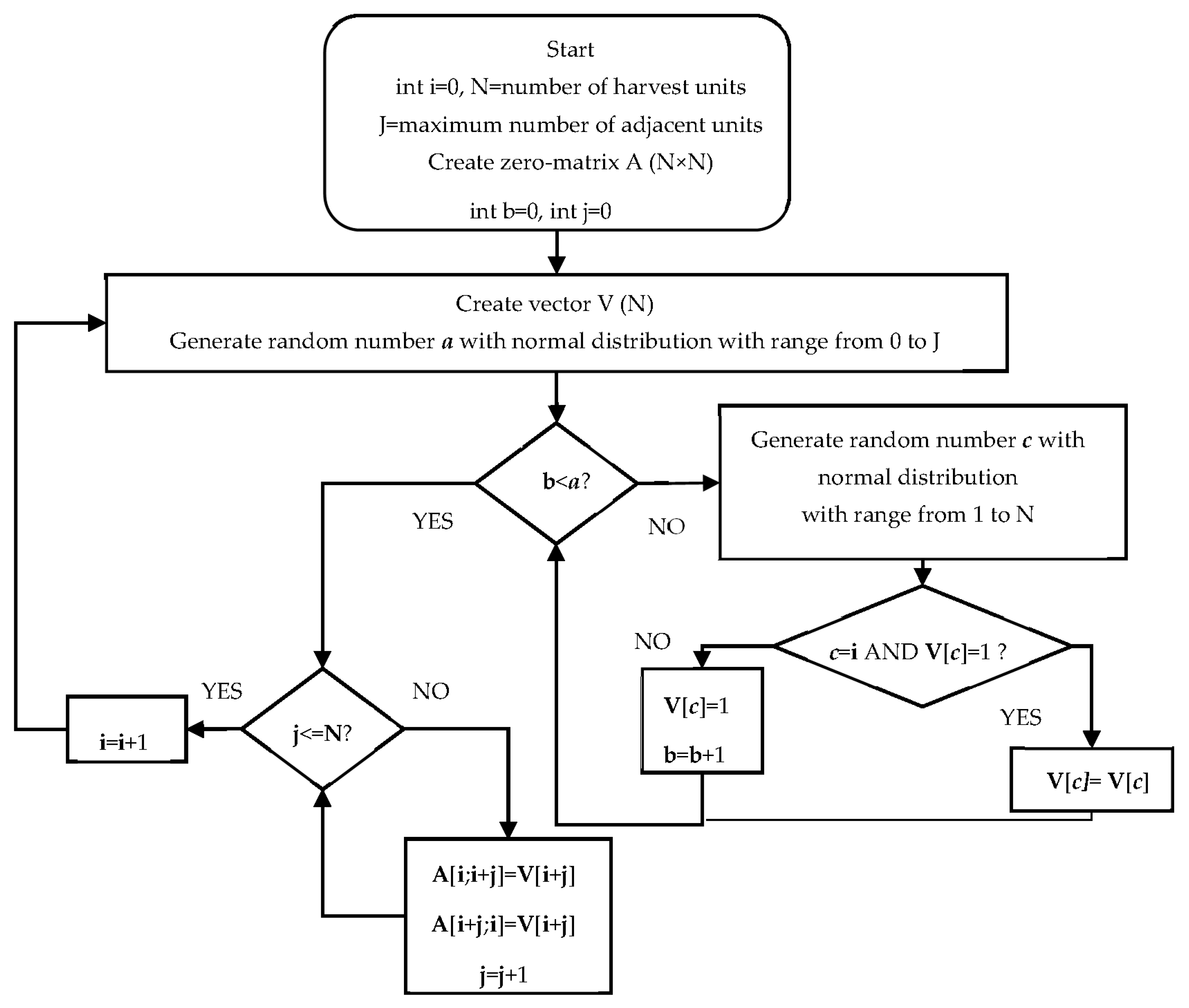
When incorporating spatial requirements into the harvest scheduling models, it is often necessary to develop algorithms for specifying adjacency constraints. The traditional algorithm for problems involving the URM model of adjacency consists of defining pairwise constraints for each harvest unit and for all adjacent units. However, this approach could be limited by a maximum possible number of constraints in commercial solving software [6]. For this reason, many researchers have tried to develop different techniques for the reduction of adjacency constraints number. A branch and bound algorithm is the most classical method of solving URM. There are two directions to reduce the size of URM with adjacency constraints. The first one is the reduction of the number of adjacency constraints, which can, however, lead to lower efficiency of a branch and bound algorithm [7]. The second one is to reformulate adjacency constraints to increase the efficiency of the branch and bound algorithm [8]. McDill and Braze [9] present five groups of adjacency constraints types that encompass 14 constraint types. Each of these types have different levels of reducing the number of constraints, which can lead to different levels of efficiency of the branch and bound algorithm.

Some authors compared the efficiency of different adjacency algorithms (see for example [10]). However, the efficiency of the algorithms is not the only crucial part of their practical utilization. There is a rapid improvement of commercial mixed integer and integer programming solvers, and hence, many solvers now accept an unlimited number of constraints [8]. Due to this, the structure of storing spatial data and creating the adjacency constraints can be the most limiting factor for practical use of decision support systems (DSS) today.

The spatial structure of forest stands or harvest units can be described using graph theory, which is applied in many fields of human activities [11,12,13]. A graph representing the adjacencies of stands or units is undirected, unweighted and can also be disconnected [13] depending on the real situation in a forest area. Although graphical representation by way of a set of vertices and edges is the most well known approach, it is not a suitable method for storing graph data in computers. For this purpose, the most common way of data storing is an adjacency matrix [11]. Another common way of data storing is an adjacency list [14]. These two graph representations have many differences that could affect the total computing time of spatially dependent forest DSSs.

The main difference between the data storing approaches is in the time of adding or deleting one edge from the vertex. In the case of the adjacency list, this time is equal to $O\left(k\right)$ where $k$ is the length of the list containing the successors of vertex $i$. In the case of the adjacency matrix, the time needed for adding or deleting one edge from the vertex is equal to $O\left(n\right)$ where $n$ is the number of vertices. This can be effective only for a very dense graph where the total number of edges $m=\mathsf{\Omega }\left(n^2\right)$ [14]. However, large numbers of adjacency relations are not very common in real forest structures [7].

The goal of this paper is to compare the time efficiency of employing the two concepts of adjacency representation, which differ in the structure of data storage and the algorithm suitable for creating constraints. The first concept is the development of conventional pairwise constraints from an adjacency list. The second concept is the development of an adjacency matrix using three analytical algorithms described by Yoshimoto and Brodie [6]. These algorithms are based on simple linear algebraic operations. The results of these comparisons should confirm or refute the following two assumptions for each selected type of adjacency constraints: (1) the number of harvest units affects the time needed to solve the model; and (2) the number of adjacent harvest units affects the time required to solve the model.

2. Materials and Methods

2.1. Model

A very simple harvest scheduling integer programing model was created for the purpose of the paper. The model is presented below (Equation (1–4)).

$$\mathit{M}\mathit{a}\mathit{x}\mathit{i}\mathit{m}\mathit{i}\mathit{z}\mathit{e}{\displaystyle {\displaystyle \sum }_{\mathit{n}=\mathbf{1}}^{\mathit{N}}}{\displaystyle {\displaystyle \sum }_{\mathit{p}=\mathbf{1}}^{\mathit{P}}}{\mathit{v}}_{\mathit{n}\mathit{p}}{\mathit{x}}_{\mathit{n}\mathit{p}}$$

(1)

subject to:

$${\displaystyle {\displaystyle \sum }_{\mathit{p}=\mathbf{1}}^{\mathit{P}}}{\mathit{x}}_{\mathit{n}\mathit{p}}\le \mathbf{1}\forall \mathit{n}\in \mathbf{1},\dots ,\mathit{I}$$

(2)

$${\mathit{x}}_{\mathit{n}\mathit{p}}+{\mathit{x}}_{\mathit{k}\mathit{p}}\le \mathbf{1}\forall \mathit{n}\in \mathbf{1},\dots ,\mathit{N},\forall \mathit{k}\in {\mathit{\Omega }}_{\mathit{n}},\forall \mathit{p}\in \mathbf{1},\dots ,\mathit{P}$$

(3a)

$$\mathbf{M}\mathbf{X}\le \mathbf{A}\mathbf{1}$$

(3b)

$${\mathit{x}}_{\mathit{n}\mathit{p}}\in \left\{\mathbf{0},\mathbf{1}\right\}$$

(4)

The objective function (1) maximizes the volume harvested from all harvest units $n=1,\dots ,N$ and from all periods $p=1,\dots ,P$, while $v_{np}$ parameter expresses the stand volume in m³. The first constraint (2) ensures that each unit is harvested only once during the planned horizon, and the second constraint (3a or 3b) is related to spatial restrictions of the problem. The set ${\mathsf{\Omega }}_n$ in inequality 3a includes all adjacent units to the unit $n$. The matrix $A$ is the adjacency matrix defined by $\left\{a_{ij}\right\},$ where $a_{ij}=1$ if unit $i$ is adjacent to unit $j$, otherwise $a_{ij}=0$; $\mathrm{X}$ is a control vector of variables $x_{np}$, $1$ is a $\left(N\times 1\right)$ unit vector, and $M$ is called a modified adjacency matrix defined by $\left\{m_{ij}\right\}$ where $m_{ij}=a_{ij}$ if $i\ne j$ and $m_{ij}=A_{i}1$ if $i=j$ (see [6] for more details).

The last constraint (4) specifies what values the decision variables $x_{np}$ can acquire. A value of $0$ means the unit $n$ is not harvested in period $p$ and $\text{is }1$ otherwise.

Using pairwise constraints does not require a special type of algorithm to define the equations. However, the original adjacency matrix of adjacency constraints (3b) can be simplified by any of the three different analytical algorithms proposed by [6]. Each is based on the symmetry of the adjacency matrix. The so-called triangular adjacency matrix (TAM) is created when the first algorithm is used. This algorithm is based on the fact that the original adjacency matrix is diagonally symmetric. The row adjacency matrix (RAM) is created using the second algorithm. Some rows in the original adjacency matrix are redundant and can be deleted. The last type of the modified adjacency matrix is the row triangular adjacency matrix (RTAM), a combination of TAM and RAM. The algorithms are specified for reduction the number of constraints. However, this can lead to lower efficiency of the branch and bound algorithm [7].

The example of an original adjacency matrix, simplified adjacency matrices of the mentioned algorithms and relevant modified adjacency matrices [6] are presented below (Equation (5–8)). The example is completely hypothetical.

Original and modified adjacency matrices without simplification	$\mathbf{A}=\left[\begin{array}{c}0100000\\ 1010000\\ 0101000\\ 0010101\\ 0001011\\ 0000100\\ 0001100\end{array}\right]$	$\mathbf{M}X=\left[\begin{array}{c}1100000\\ 1210000\\ 0121000\\ 0013001\\ 0001311\\ 0000110\\ 0001102\end{array}\right]\left[\begin{array}{c}x1\\ x2\\ x3\\ x4\\ x5\\ x6\\ x7\end{array}\right]\le \left[\begin{array}{c}1\\ 2\\ 2\\ 3\\ 3\\ 1\\ 2\end{array}\right]$	(5)
Original and modified adjacency matrices simplified by TAM	$\mathbf{A}=\left[\begin{array}{c}0000000\\ 1000000\\ 0100000\\ 0010000\\ 0001000\\ 0000100\\ 0001100\end{array}\right]$	$\mathbf{M}X=\left[\begin{array}{c}0000000\\ 1100000\\ 0110000\\ 0011000\\ 0001100\\ 0000110\\ 0001102\end{array}\right]\left[\begin{array}{c}x1\\ x2\\ x3\\ x4\\ x5\\ x6\\ x7\end{array}\right]\le \left[\begin{array}{c}0\\ 1\\ 1\\ 1\\ 1\\ 1\\ 2\end{array}\right]$	(6)
Original and modified adjacency matrices simplified by RAM	$\mathbf{A}=\left[\begin{array}{c}0000000\\ 1010000\\ 0000000\\ 0010101\\ 0000000\\ 0000100\\ 0001100\end{array}\right]$	$\mathbf{M}X=\left[\begin{array}{c}0000000\\ 1210000\\ 0000000\\ 0013101\\ 0000000\\ 0000110\\ 0001102\end{array}\right]\left[\begin{array}{c}x1\\ x2\\ x3\\ x4\\ x5\\ x6\\ x7\end{array}\right]\le \left[\begin{array}{c}0\\ 2\\ 0\\ 3\\ 0\\ 1\\ 2\end{array}\right]$	(7)
Original and modified adjacency matrices simplified by RTAM	$\mathbf{A}=\left[\begin{array}{c}0000000\\ 1010000\\ 0000000\\ 0010100\\ 0000000\\ 0000100\\ 0001100\end{array}\right]$	$\mathbf{M}X=\left[\begin{array}{c}0000000\\ 1210000\\ 0000000\\ 0012100\\ 0000000\\ 0000110\\ 0001102\end{array}\right]\left[\begin{array}{c}x1\\ x2\\ x3\\ x4\\ x5\\ x6\\ x7\end{array}\right]\le \left[\begin{array}{c}0\\ 2\\ 0\\ 2\\ 0\\ 1\\ 2\end{array}\right]$	(8)

2.2. Data

For the purpose of the paper, we consider that each harvest unit has the same stand volume in the first period. The growth multiplier of 0.05 was used for the increment in every next period. The total number of time periods in the planning horizon was 3.

Following the goal of the paper, a large number of spatial forest structures had to be used. The real spatial structures could not be used because of the input data unavailability. For this analysis, we created random adjacency matrices representing different spatial structures. The random process of generating the spatial forest structure is described in Figure 1.

The random process of generating the spatial forest structure was applied for different numbers of harvest units (N = 100 to 500) and different average number of adjacency units (J = 1 to 10). The process was repeated ten times for each combination. The 500 defined model instances were created this way. Therefore, we developed 500 random landscapes for each set of modeling assumptions. This enabled a determination of the dispersion of objective function values with respect to each combination of modeling assumptions.

Four types of adjacency constraints were generated from the adjacency matrices created using the four different approaches described above as follows: pairwise constraints and constraints from TAM, RAM and RTAM. The instances of the described model were calculated on a personal computer with Intel^® Core™ (Santa Clara, CA, USA) processor with 3.40 GHz and 16.0 GB random-access memory, which represents common computer equipment available today. The Gurobi^® version 6.0.5 (Houston, TX, USA) [15] optimization software was used with the default gap tolerance (0.01%). Two limits of solving time (60 s and 120 s) were tested. If these limits were reached, the solving process stopped. The algorithm for generating the spatial structures and for model development was programmed in the Java programming language.

The amount of time required for all model instances, the final gap tolerance for all model instances, and the number of instances solved within the time limit were measured. The total number of the resulting constraints was determined as well. The standard deviation and coefficient of variation for each common set of assumptions were calculated to understand how the solutions values might be dispersed.

3. Results

The final results of the analysis are presented in

Table 1. Solving time, gap tolerance and number of solved instances for 60 s time limit and 100 harvest units.

Number of Harvest Units	Average Number of Adjacent Units	60 s Time Limit
		Average Time (s)				Average Gap Tolerance (%)				Number of Solved Instances
		Pairwise	TAM	RAM	RTAM	Pairwise	TAM	RAM	RTAM	Pairwise	TAM	RAM	RTAM
100	0.5	0.00	0.00	0.00	0.00	0.00	0.00	0.00	0.00	10	10	10	10
	1.0	0.00	0.01	0.01	0.01	0.00	0.00	0.00	0.00	10	10	10	10
	1.5	0.00	0.01	0.01	0.02	0.00	0.00	0.00	0.00	10	10	10	10
	2.0	0.01	0.04	0.06	0.03	0.00	0.00	0.00	0.00	10	10	10	10
	2.5	0.06	0.09	0.11	0.09	0.00	0.00	0.00	0.00	10	10	10	10
	3.0	0.14	0.20	0.15	0.33	0.00	0.00	0.00	0.00	10	10	10	10
	3.5	0.48	0.78	0.55	0.79	0.00	0.00	0.00	0.00	10	10	10	10
	4.0	0.92	2.04	9.79	2.71	0.00	0.00	0.07	0.09	10	10	9	8
	4.5	2.51	11.98	9.61	25.19	0.00	0.06	0.41	0.94	10	9	6	5
	5.0	13.92	17.66	19.29	41.31	0.31	1.74	1.31	1.73	9	3	3	2

TAM = triangular adjacency matrix; RAM = row adjacency matrix; RTAM = row triangular adjacency matrix.

,

Table 2. Solving time, gap tolerance and number of solved instances for 60 s time limit and 200 harvest units.

Number of Harvest Units	Average Number of Adjacent Units	60 s Time Limit
		Average Time (s)				Average Gap Tolerance (%)				Number of Solved Instances
		Pairwise	TAM	RAM	RTAM	Pairwise	TAM	RAM	RTAM	Pairwise	TAM	RAM	RTAM
200	0.5	0.01	0.00	0.00	0.00	0.00	0.00	0.00	0.00	10	10	10	10
	1.0	0.01	0.01	0.01	0.01	0.00	0.00	0.00	0.00	10	10	10	10
	1.5	0.01	0.04	0.04	0.03	0.00	0.00	0.00	0.00	10	10	10	10
	2.0	0.09	0.17	0.14	0.16	0.00	0.00	0.00	0.00	10	10	10	10
	2.5	0.36	0.62	0.87	1.99	0.00	0.00	0.00	0.00	10	10	10	10
	3.0	2.66	8.30	9.08	19.71	0.00	0.00	0.07	0.00	10	10	7	10
	3.5	23.76	20.78	35.30	29.04	0.00	0.02	0.08	0.17	10	8	7	4
	4.0	25.31	-	31.37	-	0.14	0.61	0.88	0.78	7	0	1	0
	4.5	44.56	-	-	-	0.62	2.54	2.56	2.44	5	0	0	0
	5.0	-	-	-	-	3.06	4.58	5.31	4.18	0	0	0	0

TAM = triangular adjacency matrix; RAM = row adjacency matrix; RTAM = row triangular adjacency matrix.

,

Table 3. Solving time, gap tolerance and number of solved instances for 60 s time limit and 300 harvest units.

Number of Harvest Units	Average Number of Adjacent Units	60 s Time Limit
		Average Time (s)				Average Gap Tolerance (%)				Number of Solved Instances
		Pairwise	TAM	RAM	RTAM	Pairwise	TAM	RAM	RTAM	Pairwise	TAM	RAM	RTAM
300	0.5	0.01	0.01	0.01	0.01	0.00	0.00	0.00	0.00	10	10	10	10
	1.0	0.01	0.01	0.01	0.01	0.00	0.00	0.00	0.00	10	10	10	10
	1.5	0.02	0.05	0.05	0.05	0.00	0.00	0.00	0.00	10	10	10	10
	2.0	0.21	0.32	0.49	0.35	0.00	0.00	0.00	0.00	10	10	10	10
	2.5	2.95	15.15	9.73	8.11	0.00	0.00	0.01	0.00	10	10	9	10
	3.0	33.73	27.58	28.08	43.18	0.04	0.11	0.24	0.16	6	3	1	1
	3.5	-	-	-	-	0.22	0.38	0.60	0.44	0	0	0	0
	4.0	-	-	-	-	0.58	1.85	2.10	1.79	0	0	0	0
	4.5	-	-	-	-	2.13	3.00	3.73	2.99	0	0	0	0
	5.0	-	-	-	-	4.33	5.45	5.85	5.57	0	0	0	0

TAM = triangular adjacency matrix; RAM = row adjacency matrix; RTAM = row triangular adjacency matrix.

,

Table 4. Solving time, gap tolerance and number of solved instances for 60 s time limit and 400 harvest units.

Number of Harvest Units	Average Number of Adjacent Units	60 s Time Limit
		Average Time (s)				Average Gap Tolerance (%)				Number of Solved Instances
		Pairwise	TAM	RAM	RTAM	Pairwise	TAM	RAM	RTAM	Pairwise	TAM	RAM	RTAM
400	0.5	0.01	0.01	0.01	0.01	0.00	0.00	0.00	0.00	10	10	10	10
	1.0	0.01	0.02	0.02	0.02	0.00	0.00	0.00	0.00	10	10	10	10
	1.5	0.03	0.07	0.06	0.06	0.00	0.00	0.00	0.00	10	10	10	10
	2.0	0.28	0.72	1.35	0.58	0.00	0.00	0.00	0.00	10	10	10	10
	2.5	4.93	29.76	34.66	20.88	0.00	0.02	0.07	0.01	9	6	4	8
	3.0	-	-	-	-	0.11	0.21	0.27	0.30	0	0	0	0
	3.5	-	-	-	-	0.10	1.28	0.86	1.25	0	0	0	0
	4.0	-	-	-	-	0.36	2.34	3.00	3.20	0	0	0	0
	4.5	-	-	-	-	1.17	5.11	4.80	4.70	0	0	0	0
	5.0	-	-	-	-	5.92	8.03	7.15	7.56	0	0	0	0

TAM = triangular adjacency matrix; RAM = row adjacency matrix; RTAM = row triangular adjacency matrix.

,

Table 5. Solving time, gap tolerance and number of solved instances for 60 s time limit and 500 harvest units.

Number of Harvest Units	Average Number of Adjacent Units	60 s Time limit
		Average Time (s)				Average Gap Tolerance (%)				Number of Solved Instances
		Pairwise	TAM	RAM	RTAM	Pairwise	TAM	RAM	RTAM	Pairwise	TAM	RAM	RTAM
500	0.5	0.01	0.01	0.01	0.01	0.00	0.00	0.00	0.00	10	10	10	10
	1.0	0.01	0.02	0.03	0.03	0.00	0.00	0.00	0.00	10	10	10	10
	1.5	0.03	0.06	0.11	0.06	0.00	0.00	0.00	0.00	10	10	10	10
	2.0	0.60	5.75	1.17	1.08	0.00	0.00	0.00	0.00	10	10	10	10
	2.5	18.63	8.20	-	43.81	0.02	0.08	0.11	0.11	5	1	0	1
	3.0	-	-	-	-	0.14	0.40	0.36	0.41	0	0	0	0
	3.5	-	-	-	-	0.36	1.79	1.23	2.04	0	0	0	0
	4.0	-	-	-	-	1.98	4.04	3.27	3.56	0	0	0	0
	4.5	-	-	-	-	4.23	6.21	5.08	5.16	0	0	0	0
	5.0	-	-	-	-	6.90	7.81	8.16	8.17	0	0	0	0

TAM = triangular adjacency matrix; RAM = row adjacency matrix; RTAM = row triangular adjacency matrix.

,

Table 6. Solving time, gap tolerance and number of solved instances for 120 s time limit and 100 harvest units.

Number of Harvest Units	Average Number of Adjacent Units	120 s Time Limit
		Average Time (s)				Average Gap Tolerance (%)				Number of Solved Instances
		Pairwise	TAM	RAM	RTAM	Pairwise	TAM	RAM	RTAM	Pairwise	TAM	RAM	RTAM
100	0.5	0.00	0.00	0.00	0.00	0.00	0.00	0.00	0.00	10	10	10	10
	1.0	0.00	0.01	0.01	0.01	0.00	0.00	0.00	0.00	10	10	10	10
	1.5	0.01	0.01	0.01	0.01	0.00	0.00	0.00	0.00	10	10	10	10
	2.0	0.02	0.05	0.04	0.05	0.00	0.00	0.00	0.00	10	10	10	10
	2.5	0.07	0.08	0.11	0.08	0.00	0.00	0.00	0.00	10	10	10	10
	3.0	0.14	0.27	0.29	0.16	0.00	0.00	0.00	0.00	10	10	10	10
	3.5	0.35	0.83	1.67	1.19	0.00	0.00	0.00	0.00	10	10	10	10
	4.0	0.78	15.42	2.87	5.95	0.00	0.00	0.00	0.00	10	10	10	10
	4.5	3.41	19.48	25.42	36.51	0.00	0.24	0.10	0.00	10	9	9	10
	5.0	8.78	43.26	30.26	67.50	0.00	0.37	1.03	1.37	10	8	5	3

TAM = triangular adjacency matrix; RAM = row adjacency matrix; RTAM = row triangular adjacency matrix.

,

Table 7. Solving time, gap tolerance and number of solved instances for 120 s time limit and 200 harvest units.

Number of Harvest Units	Average Number of Adjacent Units	120 s Time Limit
		Average Time (s)				Average Gap Tolerance (%)				Number of Solved Instances
		Pairwise	TAM	RAM	RTAM	Pairwise	TAM	RAM	RTAM	Pairwise	TAM	RAM	RTAM
200	0.5	0.00	0.00	0.00	0.00	0.00	0.00	0.00	0.00	10	10	10	10
	1.0	0.00	0.01	0.01	0.01	0.00	0.00	0.00	0.00	10	10	10	10
	1.5	0.01	0.03	0.04	0.04	0.00	0.00	0.00	0.00	10	10	10	10
	2.0	0.09	0.11	0.20	0.11	0.00	0.00	0.00	0.00	10	10	10	10
	2.5	0.31	0.83	0.63	3.21	0.00	0.00	0.00	0.00	10	10	10	10
	3.0	2.49	9.07	8.46	11.19	0.00	0.00	0.03	0.00	10	10	8	10
	3.5	24.17	27.89	51.97	38.59	0.00	0.08	0.14	0.12	10	7	5	6
	4.0	34.97	77.55	-	-	0.03	0.62	0.78	0.97	9	2	0	0
	4.5	49.31	-	-	-	0.51	2.15	2.71	2.64	6	0	0	0
	5.0	-	-	-	-	2.92	3.71	4.62	3.85	0	0	0	0

TAM = triangular adjacency matrix; RAM = row adjacency matrix; RTAM = row triangular adjacency matrix.

,

Table 8. Solving time, gap tolerance and number of solved instances for 120 s time limit and 300 harvest units.

Number of Harvest Units	Average Number of Adjacent Units	120 s Time Limit
		Average Time (s)				Average Gap Tolerance (%)				Number of Solved Instances
		Pairwise	TAM	RAM	RTAM	Pairwise	TAM	RAM	RTAM	Pairwise	TAM	RAM	RTAM
300	0.5	0.00	0.01	0.01	0.01	0.00	0.00	0.00	0.00	10	10	10	10
	1.0	0.01	0.01	0.02	0.01	0.00	0.00	0.00	0.00	10	10	10	10
	1.5	0.01	0.03	0.06	0.05	0.00	0.00	0.00	0.00	10	10	10	10
	2.0	0.14	0.30	0.55	0.35	0.00	0.00	0.00	0.00	10	10	10	10
	2.5	1.09	3.96	5.48	11.29	0.00	0.00	0.01	0.01	10	10	9	9
	3.0	30.50	-	42.03	36.82	0.01	0.13	0.15	0.10	8	2	2	2
	3.5	71.49	-	-	-	0.15	0.45	0.39	0.43	1	0	0	0
	4.0	74.81	-	-	-	0.31	1.19	1.57	1.02	1	0	0	0
	4.5	-	-	-	-	1.40	3.02	3.47	3.15	0	0	0	0
	5.0	-	-	-	-	3.89	5.48	4.88	4.94	0	0	0	0

TAM = triangular adjacency matrix; RAM = row adjacency matrix; RTAM = row triangular adjacency matrix.

,

Table 9. Solving time, gap tolerance and number of solved instances for 120 s time limit and 400 harvest units.

Number of Harvest Units	Average Number of Adjacent Units	120 s Time Limit
		Average Time (s)				Average Gap Tolerance (%)				Number of Solved Instances
		Pairwise	TAM	RAM	RTAM	Pairwise	TAM	RAM	RTAM	Pairwise	TAM	RAM	RTAM
400	0.5	0.01	0.01	0.01	0.01	0.00	0.00	0.00	0.00	10	10	10	10
	1.0	0.01	0.02	0.02	0.02	0.00	0.00	0.00	0.00	10	10	10	10
	1.5	0.02	0.06	0.09	0.10	0.00	0.00	0.00	0.00	10	10	10	10
	2.0	0.37	0.79	0.92	0.95	0.00	0.00	0.00	0.00	10	10	10	10
	2.5	25.88	39.86	39.89	46.28	0.00	0.01	0.02	0.05	9	9	7	4
	3.0	51.60	-	-	-	0.08	0.19	0.27	0.24	3	0	0	0
	3.5	-	-	-	-	0.34	0.53	0.68	0.63	0	0	0	0
	4.0	-	-	-	-	0.77	1.52	1.81	1.83	0	0	0	0
	4.5	-	-	-	-	2.33	4.21	4.14	4.18	0	0	0	0
	5.0	-	-	-	-	4.71	6.76	6.33	6.09	0	0	0	0

TAM = triangular adjacency matrix; RAM = row adjacency matrix; RTAM = row triangular adjacency matrix.

and

Table 10. Solving time, gap tolerance and number of solved instances for 120 s time limit and 500 harvest units.

Number of Harvest Units	Average Number of Adjacent Units	120 s Time Limit
		Average Time (s)				Average Gap Tolerance (%)				Number of Solved Instances
		Pairwise	TAM	RAM	RTAM	Pairwise	TAM	RAM	RTAM	Pairwise	TAM	RAM	RTAM
500	0.5	0.01	0.01	0.01	0.01	0.00	0.00	0.00	0.00	10	10	10	10
	1.0	0.01	0.03	0.03	0.03	0.00	0.00	0.00	0.00	10	10	10	10
	1.5	0.03	0.08	0.11	0.10	0.00	0.00	0.00	0.00	10	10	10	10
	2.0	0.65	0.95	2.47	1.76	0.00	0.00	0.00	0.00	10	10	10	10
	2.5	51.64	75.65	61.45	32.58	0.03	0.00	0.05	0.00	3	3	3	1
	3.0	-	-	-	-	0.14	0.27	0.35	0.38	0	0	0	0
	3.5	-	-	-	-	0.38	0.88	1.18	0.92	0	0	0	0
	4.0	-	-	-	-	1.12	2.61	3.22	3.09	0	0	0	0
	4.5	-	-	-	-	3.83	5.08	4.76	5.24	0	0	0	0
	5.0	-	-	-	-	5.52	8.23	7.44	7.71	0	0	0	0

TAM = triangular adjacency matrix; RAM = row adjacency matrix; RTAM = row triangular adjacency matrix.

. The calculated average values of the solution time required, the final gap tolerance characteristics, and the number of solved instances in the case of the 60 s and 120 s solving time limit are presented in Table 1, Table 2, Table 3, Table 4 and Table 5 (100, 200, 300, 400 and 500 harvest units) and Table 6, Table 7, Table 8, Table 9 and Table 10 (100, 200, 300, 400 and 500 harvest units), respectively.

In Table 1, we see that nearly all (9 of 10) attempts to solve the problem using pairwise constraints were successful for all assumptions of the number of adjacent neighbors. This problem only involved 100 stands, yet several formulations using the TAM, RAM, and RTAM adjacency matrices were unable to be solved in 60 s. From Table 2, Table 3, Table 4 and Table 5, we see that the different constraint formulations prevent the problem described in this research from being solved within 60 s when the number of stands assumed increases. In this case, when the number of stands increased to 200, none of the formulations with 5 adjacent stands on average were able to be solved in 60 s. Table 3 suggests that a problem with 3 or more (on average) adjacency relationships associated with 300 stands is not solvable in 60 s using any of the methods employed in this research. Table 4, when 400 stands are modeled, suggests that only problems with 2.5 adjacent stands (on average) can be solved in 60 s. The results in Table 5 are similar, when 500 stands are modeled, yet the problems with pairwise constraints were the only ones somewhat consistently solved in 60 s. In this case, however, only 5 of 10 attempts were solved. In each case, the smallest optimality gap (on average) was observed when using the pairwise constraints.

In Table 6, we see that all 10 attempts to solve the problem using pairwise constraints were successful for all assumptions of the number of adjacent neighbors. This problem only involved 100 stands, yet several formulations using the TAM, RAM, and RTAM adjacency matrices were unable to be solved in 120 s. From Table 7 onward, we begin to see that the different constraint formulations prevent the problem described in this research from being solved within 120 s when the number of stands assumed increases. Here, when the number of stands increased to 200, none of the formulations with 5 adjacent stands on average were able to be solved in 120 s. In Table 8, one can see that the pairwise constraint formulation was able to solve the problem (1 of 10 times) in 120 s when 300 stands were modeled and the average number of adjacent stands was 3.5 or 4. The other constraint formulations seemed to require more than 120 s in these cases. In Table 9, one can see that the pairwise constraint formulation was the only one of the four tested that was able to solve the problem (3 of 10 times) in 120 s when 400 stands were modeled and the average number of adjacent stands was 3. Table 10 suggests that a problem with 3 or more (on average) adjacency relationships associated with 500 stands is not solvable in 120 s, using any of the methods employed in this research.

It is clear from the tables that the complexity of the model instances increases not only with the number of harvest units but also with the average number of the adjacent harvest units. This fact can be seen in the behavior of all three measured characteristics for all four different types of adjacency constraints. It can also be proclaimed that with the increasing complexity of the model instances, the solution time and the final gap tolerance (the lower the gap tolerance, the better the result) also increase, while the number of model instances solved under the time limit decreases.

The calculated standard deviations and coefficients of variation of solving time for all combinations are presented in

Table 11. Resulting standard deviation (SD) and coefficient of variation (CV) of solving time for 60 s time limit.

Num. of Harvest Units	Average Number of Adjacent Units	60 s Time Limit
		Pairwise		TAM		RAM		RTAM
		SD	CV	SD	CV	SD	CV	SD	CV
100	0.5	0.001	22.71	0.001	19.71	0.001	23.29	0.001	21.53
	1.0	0.001	28.67	0.002	30.95	0.001	22.97	0.001	13.66
	1.5	0.002	37.79	0.009	66.90	0.004	31.75	0.008	48.82
	2.0	0.005	39.49	0.022	49.81	0.021	36.74	0.010	31.77
	2.5	0.035	58.22	0.040	46.27	0.037	33.79	0.024	28.07
	3.0	0.091	63.44	0.117	58.04	0.089	58.09	0.432	130.98
	3.5	0.514	106.27	0.767	98.84	0.612	112.06	0.971	122.48
	4.0	1.425	155.34	1.575	77.04	17.356	177.36	2.666	98.53
	4.5	1.918	76.49	17.611	147.04	5.010	52.16	26.128	103.72
	5.0	12.087	86.85	18.046	102.20	7.841	40.66	-	-
200	0.5	0.001	18.28	0.001	25.30	0.001	22.58	0.001	19.64
	1.0	0.001	19.56	0.001	10.20	0.002	17.08	0.001	12.66
	1.5	0.007	50.41	0.040	109.16	0.034	77.52	0.017	56.61
	2.0	0.055	64.04	0.061	34.96	0.049	33.99	0.038	23.81
	2.5	0.178	49.11	0.614	98.66	0.572	65.63	3.392	170.35
	3.0	3.374	126.75	8.927	107.62	6.952	76.54	18.389	93.32
	3.5	7.909	33.29	7.498	36.09	19.082	54.06	22.970	79.11
	4.0	10.832	42.80	-	-	-	-	-	-
	4.5	18.384	41.26	-	-	-	-	-	-
300	0.5	0.001	15.15	0.001	25.58	0.001	25.55	0.001	17.82
	1.0	0.000	4.79	0.002	14.34	0.003	17.64	0.002	12.94
	1.5	0.009	50.12	0.041	82.30	0.017	34.79	0.038	70.28
	2.0	0.086	41.24	0.219	68.38	0.320	65.16	0.199	56.49
	2.5	4.472	151.83	18.135	119.71	16.912	173.80	7.012	86.47
	3.0	22.721	67.36	7.515	27.25	-	-	-	-
400	0.5	0.000	6.57	0.001	18.25	0.001	13.05	0.000	6.48
	1.0	0.001	5.72	0.002	11.78	0.002	10.31	0.002	12.05
	1.5	0.020	76.72	0.062	84.90	0.020	33.09	0.052	80.99
	2.0	0.268	96.69	0.503	69.64	1.115	82.66	0.451	77.39
	2.5	3.486	70.71	15.037	50.53	19.588	56.51	10.618	50.86
500	0.5	0.002	20.98	0.001	14.60	0.001	11.49	0.001	15.86
	1.0	0.003	22.92	0.002	8.80	0.004	16.72	0.002	9.53
	1.5	0.016	50.72	0.009	16.46	0.068	60.79	0.028	43.19
	2.0	0.377	62.67	13.444	233.92	0.716	61.13	0.579	53.73
	2.5	18.413	98.81	-	-	-	-	-	-

Note: If one could not achieve the results by any algorithm (pairwise, TAM, RAM, RTAM), it means all values were discredited. TAM = triangular adjacency matrix; RAM = row adjacency matrix; RTAM = row triangular adjacency matrix; SD = standard deviation; CV = coefficient of variation.

and

Table 12. Resulting standard deviation (SD) and coefficient of variation (CV) of solving time for 120 s time limit.

Num. of Harvest Units	Average Number of Adjacent Units	120 s Time Limit
		Pairwise		TAM		RAM		RTAM
		SD	CV	SD	CV	SD	CV	SD	CV
100	0.5	0.000	13.74	0.001	22.69	0.001	20.47	0.001	17.91
	1.0	0.000	8.38	0.001	18.30	0.002	28.97	0.001	14.64
	1.5	0.002	34.07	0.002	18.73	0.007	50.42	0.006	45.25
	2.0	0.016	82.97	0.032	63.00	0.031	69.78	0.026	51.48
	2.5	0.046	70.67	0.045	54.52	0.032	30.33	0.017	21.70
	3.0	0.045	33.12	0.273	102.55	0.405	137.81	0.096	61.43
	3.5	0.196	55.84	1.246	149.45	2.391	143.35	1.403	117.55
	4.0	0.868	111.53	20.973	136.00	3.496	121.94	9.187	154.48
	4.5	1.863	54.57	26.337	135.18	42.423	121.64	36.784	100.76
	5.0	5.634	64.14	27.493	63.55	57.093	76.00	44.420	65.80
200	0.5	0.001	19.58	0.001	23.36	0.001	22.47	0.001	20.98
	1.0	0.000	7.70	0.002	21.36	0.001	10.49	0.005	40.46
	1.5	0.007	72.68	0.027	89.44	0.031	74.21	0.027	69.58
	2.0	0.081	88.21	0.054	49.04	0.139	68.14	0.056	48.62
	2.5	0.109	35.73	0.747	90.11	0.577	91.60	8.176	255.08
	3.0	1.719	69.12	8.784	96.88	47.533	562.06	9.554	85.35
	3.5	18.903	78.22	44.796	160.59	37.452	72.07	28.349	73.47
	4.0	34.588	98.92	-	-	-	-	-	-
	4.5	6.552	13.29	-	-	-	-	-	-
300	0.5	0.000	7.02	0.001	24.10	0.001	12.28	0.001	14.30
	1.0	0.002	30.64	0.002	16.41	0.002	14.51	0.003	17.10
	1.5	0.005	41.89	0.013	39.24	0.046	75.31	0.024	48.24
	2.0	0.147	105.69	0.127	42.05	0.417	75.40	0.214	60.92
	2.5	0.792	72.52	7.864	198.57	36.789	671.39	35.097	310.88
	3.0	25.937	85.04	14.713	-	-	-	-	-
400	0.5	0.001	10.78	0.001	17.72	0.001	12.40	0.001	10.95
	1.0	0.002	20.32	0.003	15.01	0.005	25.23	0.003	14.73
	1.5	0.016	64.17	0.049	78.61	0.070	80.37	0.060	60.40
	2.0	0.300	80.17	0.818	102.94	1.014	110.74	0.836	88.30
	2.5	36.264	140.13	44.675	112.08	19.493	48.87	21.056	45.50
	3.0	21.129	40.95	-	-	-	-	-	-
500	0.5	0.000	5.41	0.002	17.68	0.001	13.63	0.001	10.55
	1.0	0.001	5.37	0.006	25.52	0.003	10.29	0.006	23.11
	1.5	0.014	39.88	0.047	60.35	0.084	78.09	0.094	92.46
	2.0	0.374	57.30	0.584	61.75	2.621	105.95	2.821	160.71
	2.5	46.615	90.26	-	-	48.235	78.50	-	-

Note: If one could not achieve the results by any algorithm (pairwise, TAM, RAM, RTAM), it means all values were discredited. TAM = triangular adjacency matrix; RAM = row adjacency matrix; RTAM = row triangular adjacency matrix; SD = standard deviation; CV = coefficient of variation.

. One can observe that the higher complexity of model instance is coupled with higher standard deviation and coefficient of variation of solving time. Unfortunately, the lower number of solved model instances in some cases may cause discredit of the calculated values. In addition, it is shown in previous tables that the chances to solve the various models in real time decrease with increases in the model complexity. The results are not surprising, since a time limit applied to more complex models does not allow the branch and bound algorithm to sufficiently search the solution space. Therefore, the solutions reported after 60 or 120 s are expectedly sub-optimal, leading to greater variation in the sample objective function values.

Only in the case of very simple spatial structures (where the average number of adjacent units ranges from 0.5 to 2.0 units), all four types of adjacency constraints had the same effect on the solving time, gap tolerance, and number of solved instances within the time limit (Table 1, Table 2, Table 3, Table 4, Table 5, Table 6, Table 7, Table 8, Table 9 and Table 10). These very simple spatial structures can represent forest management areas with very low density of mature forests stands.

The pairwise adjacency constraints were more successful in solving most instances than other types of adjacency constraints. Even in the cases when the average time of solving was greater, the final gap tolerance was lower or the number of solved instances within the time limit was higher. Even in spite of the really low number of constraints obtained by TAM, RAM and RTAM (

Table 13. Resulting number of adjacency constraints obtained by different algorithms for different types of spatial forest structures.

Number of Harvest Units	Average Number of Adjacent Units	Pairwise	TAM	RAM	RTAM
100	0.5	49	21	19	19
	5.0	496	80	64	64
200	0.5	94	41	37	37
	5.0	1012	162	130	128
300	0.5	153	66	57	56
	5.0	1484	242	194	195
400	0.5	198	85	76	75
	5.0	1981	323	256	256
500	0.5	248	108	98	95
	5.0	2476	403	323	322

TAM = triangular adjacency matrix; RAM = row adjacency matrix; RTAM = row triangular adjacency matrix.

), the pairwise constraints were more successful in solving these problems in a timely manner.

4. Discussion

Without adjacency restrictions represented by adjacency constraints in a harvest scheduling model, a forest manager cannot be sure that the results of such a model are feasible in real management situations. However, these constraints can dramatically complicate the process of developing a forest plan [10], especially in the case of small-scale unit restriction models. In our case, the maximum area of each harvest unit was not to exceed 2 hectares (yet could be 1 hectare in some countries), which represents a very common planning situation in Central Europe. In other areas of the world, this scale of problem could be similar to the arrangement and scheduling of group selection harvest patches, where the patches should not touch within a given time frame in order to maintain the patch size suggested in the silvicultural system [16]. In either case, the small-scale unit restriction problem is a microcosm of larger-scale adjacency issues that involve restricting the maximum final harvest size (e.g., 50 ha) within a given green-up period.

At the beginning of the computer-based spatial harvest scheduling in 1990’s, it was possible to solve only small scheduling problems (i.e., small number of decision variables and constraints) because of the limitations of personal computers and solvers. However, increasing computing speeds and improved commercial solvers enable us to solve larger and larger problems [8]. It is generally known that the power of computers has been growing exponentially, and solvers have also been dramatically improved. In connection with this, the use of forest harvest scheduling DSSs has also dramatically increased. For this reason, researchers should periodically re-analyze different practical and theoretical aspects of harvest scheduling models. This service to society allows knowledge of the capabilities of forest planning systems to grow and to become adapted within forest management organizations.

Few scientific papers have dealt with the effect of reducing the number of adjacency constraints by different methods (see for example [6,7,17]). The number of adjacency constraints can be significantly reduced as is confirmed and presented in this paper. This is especially true in the case of large problems with complex spatial structures. As the number of constraints is reduced within a complex planning problem, one would hope that the time required to solve the problem would also be reduced. We have confirmed this hypothesis as well for the problem instances that were examined in this work. Therefore, our contribution incrementally adds to the body of science associated with applied optimization in this respect.

One of the first papers dealing with measuring the efficiency of adjacency constraints was presented by Murray and Church [18]. They tested several different types of adjacency constraints including pairwise constraints and TAM constraints presented above. The results of their analyses showed that TAM had the lowest efficiency, which was also confirmed in this paper. Tóth et al. [19] explored strengthening procedures for improving adjacency formulations of the area restriction forest planning problem. These efforts underscore the need to expand science in this area through the development and analysis of new methods for addressing practical forest management problems. Our work complements and adds to the growing body of science, yet due to the various types of forest management problems encountered around the world, by no means represents the final word on the subject. As the expectations of society evolve, the decision space within which forest managers can operate changes. Therefore, we expect novel and creative methods for combinatorial problems will continue to be assessed in association with efforts aimed at sustainable forest management.

The solving time and the final gap tolerance were also analyzed by McDill and Braze [10]. The authors randomly generated hypothetical forests of four different age structures. They tested three types of adjacency constraints: pairwise constraints, Type I constraints (encompassing several methods leading to the same results and proposed by many authors) and NOAM constraints based on the adjacency matrix proposed by Murray and Church [20]. The authors achieved the best results with Type I constraints. This fact could not be confirmed or confuted by the results presented here, although the algorithm based on the adjacency matrix had longer solution time as was presented before in the Results section. This means that adjacency matrix algorithms do not have to be an optimal approach for defining the adjacency relationships. On the other hand, the authors used another solver (CPLEX^® (Armonk, NY, USA)) and also a different type of computer, of which the latter is already outdated. It is questionable if the results would be the same with currently used computers and software.

The solving time of harvest scheduling models is dependent not only on the inherent spatial forest structure, but also on the number of planning periods, the length of each period, other types of constraints related to the planning problem (e.g., a type of harvest flow constraints), the computer employed, the software employed and its settings [21]. The input age structure can affect the model complexity [9]. The evaluation of the effects of all these aspects was not the aim of this study. We focused on the types of adjacency constraints, which are used in the DSS called Optimal [22,23]. Other mentioned aspects should be analyzed individually in more detail.

As we stated before, one aspect of different types of adjacency constraints that has not been studied yet, though it has an impact on real-life scheduling situations, is their consumption of computer random-access memory. The consumption of memory can limit using DSSs aimed at spatial harvest scheduling, for instance Optimal or Heureka [24]. In these cases, adjacency constraints can be created directly from a database, in which the spatial information is saved in the form of pairwise adjacency constraints. However, all spatial information must be uploaded to the computer memory at first, and kept in the memory during the algebraic process when using the presented analytical algorithms. Therefore, the amount of memory used to manage the data may take away memory available to a solver in developing a forest plan. This may have varying effects on the ability and time required to solve a problem, and likely depends on the data, computer, and software at the disposal of the forest planner.

Following the assumptions we stated in the Introduction, we can confirm that the number of harvest units affects the solving time of model instances, although the number of adjacent units has a greater effect. On the basis of the presented results, we can recommend using the pairwise type of adjacency constraints for solving unit restriction harvest scheduling models.

5. Conclusions

We presented an analysis of four different types of adjacency constraints used for solving unit restriction harvest scheduling models. The first type was a traditional type of pairwise constraints, while the other three types were adjacency constraints defined by three different analytical algorithms. These algorithms were developed to reduce the total number of adjacency constraints, which can be much greater in comparison to pairwise constraints. However, the reduction of constraints can decrease the efficiency of branch and bound based algorithms, regardless of the demand for the greater computer random-access memory consumption. As was shown, the reduction of constraints may no longer be needed, because today’s solvers are not limited by the number of constraints and the traditional pairwise adjacency constraints are more effective for solving spatial harvest scheduling models.

References

1. Dykstra, D.P. Mathematical Programming for Natural Resource Management; McGraw-Hill Book Company Inc.: New York, NY, USA, 1984. [Google Scholar]
2. Baskent, E.Z.; Keles, S. Spatial forest planning: A review. Ecol. Model 2005, 188, 145–173. [Google Scholar] [CrossRef]
3. Kurtilla, M. The spatial structure of forests in the optimization calculations forest planning—A landscape ecological perspective. For. Ecol. Manag. 2001, 142, 129–142. [Google Scholar] [CrossRef]
4. Murray, A.T. Spatial restrictions in harvest-scheduling. For. Sci. 1999, 45, 45–52. [Google Scholar]
5. Jamnick, M.S.; Walters, K.R. Spatial and temporal allocation of stratum-based harvest schedules. Can. J. For. Res. 1993, 23, 402–413. [Google Scholar] [CrossRef]
6. Yoshimoto, A.; Brodie, J.D. Comparative analysis of algorithms to generate adjacency constraints. Can. J. For. Res. 1994, 24, 1277–1288. [Google Scholar] [CrossRef]
7. Torres-Rojo, J.M.; Brodie, J.D. Adjacency constraints in harvest scheduling: An aggregation heuristic. Can. J. For. Res. 1990, 20, 978–986. [Google Scholar] [CrossRef]
8. Crowe, K.; Nelson, J.; Boyland, M. Solving the area-restricted harvest-scheduling model using the branch and bound algorithm. Can. J. For. Res. 2003, 33, 1804–1814. [Google Scholar] [CrossRef]
9. McDill, M.E.; Braze, J. Comparing adjacency constraint formulations for randomly generated forest planning problems with four age-class distributions. For. Sci. 2000, 46, 423–436. [Google Scholar]
10. McDill, M.E.; Braze, J. Using the branch and bound algorithm to solve forest planning problems with adjacency constraints. For. Sci. 2000, 47, 403–418. [Google Scholar]
11. Bondy, J.A.; Murty, U.S.R. Graduate Texts in Mathematics; Springer-Verlag Heidelberg: New York, NY, USA, 2000. [Google Scholar]
12. Diestel, R. Graph Theory, 3rd ed.; Springer-Verlag Heidelberg: New York, NY, USA, 2005. [Google Scholar]
13. Benjamin, A.; Chartrand, G.; Zhang, P. The Fascinating World of Graph Theory; Princeton University Press: Princeton, NJ, USA, 2015. [Google Scholar]
14. Mehlhorn, K.; Sanders, P. Algorithms and Data Structure—The Basic Toolbox; Springer-Verlag: Berlin/Heidelberg, Germany, 2008. [Google Scholar]
15. Gurobi Optimizer Reference Manual 6.5. Available online: http://www.gurobi.com/documentation/6.5/refman/java_api_overview.html#sec:Java (accessed on 1 December 2015).
16. Bettinger, P.; Johnson, D.L.; Johnson, K.N. Spatial forest plan development with ecological and economic goals. Ecol. Model 2003, 169, 215–236. [Google Scholar] [CrossRef]
17. Hoganson, H.M.; Borges, J.G. Using dynamic programming and overlapping subproblems to address adjacency in large harvest scheduling problems. For. Sci. 1998, 44, 526–538. [Google Scholar]
18. Murray, A.T.; Church, R.L. Measuring the efficacy of adjacency constraint structure in forest planning models. Can. J. For. Res. 1995, 25, 1416–1424. [Google Scholar] [CrossRef]
19. Tóth, S.F.; McDill, M.E.; Könnyű, N.; George, S. A strengthening procedure for the path formulation of the area-based adjacency problem in harvest scheduling models. Math. Comput. For. Nat. Res. Sci. 2012, 4, 27–49. [Google Scholar]
20. Murray, A.T.; Church, R.L. Constructing and selecting adjacency constraints. INFOR 1996, 34, 232–248. [Google Scholar]
21. Snyder, S.; ReVelle, C. Dynamic selection of harvest units with adjacency restrictions: The SHARe model. For. Sci. 1997, 43, 213–222. [Google Scholar]
22. Marušák, R.; Kašpar, J.; Vopěnka, P. Decision support system (DSS) optimal—A case study from the Czech Republic. Forests 2015, 6, 163–182. [Google Scholar] [CrossRef]
23. Vopěnka, P.; Kašpar, J.; Marušák, R. GIS tool for optimization of forest harvest-scheduling. Comput. Electron. Agric. 2015, 113, 254–259. [Google Scholar] [CrossRef]
24. Wikstrӧm, P.; Edenius, L.; Elfving, B.; Eriksson, L.O.; Lämås, T.; Sonesson, J.; Ӧhman, K.; Wallerman, J.; Waller, C.; Klintebäck, F. The heureka forestry decision support system: An overview. Math. Comput. For. Nat. Res. Sci. 2011, 3, 87–95. [Google Scholar]
Figure 1. The process of random generation of a spatial forest structure (int = integer number).
Forests 07 00102 g001