Article

Evaluation of Image-Assisted Forest Monitoring: A Simulation

by
Francis A. Roesch
1,*,
John W. Coulston
2,
Paul C. Van Deusen
3 and
Rafał Podlaski
4
1
Southern Research Station, USDA Forest Service, 200 WT Weaver Blvd. Asheville, NC 28804, USA
2
Southern Research Station, USDA Forest Service, 1710 Research Center Drive, Blacksburg, VA 24060, USA
3
National Council for Air and Stream Improvement (NCASI), 60 East St., Mount Washington, MA 01258, USA
4
Department of Nature Protection, Institute of Biology, Jan Kochanowski University, ul. Świętokrzyska 15, Kielce 25-406, Poland
*
Author to whom correspondence should be addressed.
Forests 2015, 6(9), 2897-2917; https://doi.org/10.3390/f6092897
Submission received: 21 May 2015 / Revised: 6 August 2015 / Accepted: 17 August 2015 / Published: 25 August 2015

Abstract

:
Fiscal uncertainties can sometimes affect national continuous forest monitoring efforts. One solution of interest is to lengthen the time it takes to collect a “full set” of plot data from five to 10 years in order to reduce costs. Here, we investigate using ancillary information to partially offset this proposed solution’s negative effects. We focus our discussion on the corresponding number of years between measurements of each plot while we investigate how thoroughly the detrimental effects of the reduced sampling effort can be ameliorated with change estimates obtained from temporally-dense remotely-sensed images. We simulate measured plot data under four sampling error structures, and we simulate remotely-sensed change estimates under three reliability assumptions, integrated with assumptions about the additional unobserved growth resulting from the lengthened observation window. We investigate a number of estimation systems with respect to their ability to provide compatible annual estimates of the components of change during years spanned by at least half of the full set of plot observations. We show that auxiliary data with shorter observation intervals can contribute to a significant improvement in estimation.

1. Introduction

Fiscal uncertainties can sometimes affect national continuous forest monitoring efforts. The sample designs for these large long-term efforts are often inflexible and can be adversely affected by budget shortfalls. When a budget shortfall affects a national forest inventory (NFI) program to the extent that it reduces the interpretive ability of the effort, the effects can be wide-ranging and profound. For instance, in Europe, there has been a concerted effort to interpret multiple national forest inventories, in unison, in order to understand continent-wide (and world-wide) forest population change by harmonizing monitoring information at the supra-national level (e.g., Tomppo and Schadauer [1]). This harmonization process, as well as monitoring forest population change in general, can be hampered severely by national budget shortfalls, which are occurring with increasing frequency. A further complication lies in the fact that limitations of capital expenses can be very different in different countries. This has led to many different solutions for the problem. In some cases, the scope and objectives of the monitoring have been limited by strategies involving a reduction of the number of sample plots or an increase in the number of years between measurements of the sample plots. Decreasing the number of the plots might be effected randomly over the entire area covered by a particular monitoring effort or it might be restricted to areas considered to be of minor economic or managerial significance. Reducing the scope or objectives of the monitoring effort can result in the collection of a reduced set of variables or in fewer measurements of a particular variable. For instance, because the measurement of tree height can be very time consuming, limiting the number of tree height measurements is often one of the effected solutions. Increasing the number of years between measurements of sample plots can involve all of the plots or only the plots in particular subpopulations. In addition, a staggered measurement schedule might be incorporated, such as measuring 50% of the plots in one measurement year and the remaining 50% of the plots in another one. By this scheme, the number of years between measurements of each set of plots might remain unchanged. An extension of this idea, which was intended to result in annually-consistent budgets, led to the United States Department of Agriculture (USDA) Forest Service’s panelized annual inventory system conducted by the Forest Inventory and Analysis (FIA) Program. Even with this level of budgetary planning, further shortfalls can occur. Here, we investigate the effects of one proposed solution to a potential budget shortfall for the national monitoring effort conducted by FIA. The solution of interest is to lengthen the “cycle”, that is the time it takes to collect a “full set” of plot data from five years to 10 years. This solution can have manifold implications, a few of which have been discussed in Roesch [2] and Roesch and Van Deusen [3].
We use a simulation to investigate how thoroughly the detrimental effects of the reduced sampling effort can be ameliorated with change estimates obtained from temporally-dense remotely-sensed images. Within the simulation, we use four sampling error structures for the measured plot data and three assumptions of applicability of the remotely-sensed image change estimates (ICE).
Specifically, our objective is to obtain annual estimates of the components of change, given multi-year data collected by temporally-overlapping panels. Van Deusen and Roesch [4] and Roesch and Van Deusen [5] explored estimation of the change in forest land classification, in the context of the national forest inventory in the United States, while Roesch [6] concentrated on estimation of the change in the tree population on land that remains forested throughout the period of interest. The current work focuses on land that is forested at some point during a period of interest. Eriksson [7] presented a set of definitions for the continuous components of change. In this paper, we subscribe to the definitions of Roesch [8], which presented a discrete version of the Eriksson definitions. We define entry as the cubic meter volume (or value) of trees as they attain the entry criterion; live growth as the annual growth in volume that occurs on trees after a defined entry criterion has been achieved; mortality as the volume of trees as they die; and harvest as the volume of trees as they are harvested.
These population components of change are compatible, that is:
Y t + 1 = Y t + L t + E t M t H t
where:
  • Yt = the value of interest at the beginning of year t;
  • Lt = growth in the value of interest on live trees during year t;
  • Et = the value of interest on live trees as they enter the population during year t;
  • Mt = the value of interest on trees as they die during year t and;
  • Ht = the value of interest on trees as they are harvested during year t.
It has often been argued that because these components are compatible, the estimators of these components should also be compatible. The recursive estimation systems that we explore here are compatible and are compared to non-recursive estimation systems. For clarity and without loss of generality, assume that the estimands of interest are the cubic meter volume per hectare of all live trees in a fixed area in each component of change category during each year of a multi-decadal period. The plot sampling design considered here consists of a number (g) of mutually-exclusive, spatially-disjoint and temporally-successive panels. The first panel to be measured is selected by locating a random point within the population area. One panel per year is then measured, in a predetermined order of succession, for g years. After the entire set of panels has been measured, the sequence reinitiates. Bechtold and Patterson [9] discuss an example of this type of design. Various statistical aspects of this type of design have been discussed by McCollum [10], Van Deusen [11], Roesch et al. [12] and Van Deusen [13], among others. This panel design provides remeasurement observations that are spatially disjoint and temporally overlapping. Usually, analysts are interested in a temporal scale that is finer than the scale of observation, which has resulted in a number of suggestions for obtaining those finer-scale estimates. Roesch [8] argued that the average annual growth within each individual panel is best applied to the center of the measurement interval, which is analogous to an assumption of linear change between observations. This was thought to be a reasonable first approximation, in lieu of contradictory evidence. All analytical methods proposed to date for this class of forest monitoring sample designs have been predicated on this or similar assumptions. For the interested reader, a related discussion can be found in Westfall et al. [14].
Roesch and Van Deusen [3] discussed the effects of ignoring differences in the temporal aspects of a realized sample from the intended design. Specifically, they showed the effects of two (usually tacit) assumptions in NFI designs. The first was that variation in the time of observation for an individual areal sample is ignorable. The second was that variation in the remeasurement period lengths between individual plots in successive areal samples was ignorable. They explored the effects of these assumptions and discussed how inference can be improved by a judicious accounting of these sampling disparities. They showed the remeasurement period assumption to be especially problematic. That is, plots in NFI systems are never remeasured on exact temporal intervals, and large biases can be introduced when there is little effort made to restrict the distribution of temporal interval lengths. They concluded that further research was needed to determine what restrictions should be placed on the distribution of temporal intervals to achieve specific objectives. This paper constitutes one specific extension of that research in that we explore some of the effects of an unusually-long survey cycle.

2. Methods

2.1. Simulated Population

To construct the simulated population, we used methods similar to those used to construct one of the populations in Roesch [6], specifically Population 1 in the referenced work. We started with the FIA plot data measured at least twice by the annual sample design in the state of Georgia (USA) between 1995 and 2012. This resulted in 7330 plots, most of which had 3 measurement times (i.e., two observed growth intervals for each component). Note that although the FIA sample design includes a plot remeasurement interval of 5 years, logistical adjustments, especially in the early years of usage of the design, led to the actual remeasurement interval varying quite widely around the 5-year target for these plots. To create a plausible population, we first created a seed population (Population 0) utilizing the theory and methods described in Roesch [6] for deriving annual values from the multi-year observations. The seed population allowed us to simulate a population (Population 1), from which we might assume the observed sample data could have been drawn. Because exact harvest times were unknown, harvested volume was randomly allocated to a year within each observation interval. Linear interpolation and extrapolation were used to obtain an initial value for the live growth, entry and mortality change components for each year from 1995 through 2012, as well as a starting cubic-meter per hectare value in the beginning of 1995, with temporal adjustments made as necessary for high levels of harvest and mortality (note that, as in Roesch [6], we are not attempting to reconstruct the plot, but rather a reasonable facsimile to the forested condition from which it could have been drawn). Construction of Population 0 then proceeded with 500 variance-interjected copies of Set 1, resulting in 3,665,000 hectares, 2,360,411 of which were forested at some time during the period of interest. The population is represented by 5 matrices, each with 3,665,000 rows and 18 columns (one column for each year), one matrix for each change component and one for initial annual volume. Variance was interjected at two levels. In Level 1, to maintain the trend while adding variance to the seed, all values for each component on each hectare were multiplied by a unique random variate, drawn from an N (1, 0.025) distribution. The second level of variance was introduced temporally by multiplying the result of Step 1 for each annual value for each component on each hectare by a unique random variate drawn from an N (1, 0.0025) distribution, thereby completing the construction of Population 0. For Population 1, a mild (latent) non-linear trend was introduced into each of the components of Population 0, T 1 i = [ 0.95 + ( 0.05 l n ( i 1997 ) ) ] ,   i = 1998   to   2011 , where each value in each year i is multiplied by T1i. Table 1 gives the Population 1 distribution statistics for 1998 to 2011. Population 1 is available from the first author upon request.

2.2. Sampling Simulations

Each simulation consisted of 1000 iterations of 1000 plots each (without replacement) from each population, under each of the four sampling error structures. In the current investigation, we use a method similar to that described in Roesch [6], to consider 4 sampling error structures. The sampling errors used here are elevated relative to those described in Roesch [6] in order to account for additional errors resulting from the longer cycle length or observation window. Note that the use of the sampling error structures to account for unobserved live growth should be greater for a 10-year observation window than for a 5-year observation window. This affects all live growth on mortality and cut trees between the last observation and the time of death or harvest. Therefore, the components of live growth, mortality, and harvest are more heavily affected by this additional error than entry. The entry component is affected by the cohort of trees that entered the population and died or were harvested prior to the next observation.
Each of the four sampling error structures was introduced by multiplying a unique random normal deviate of mean b and standard deviation d from Table 2 by each sampled observation of initial volume, entry, live growth, mortality and harvest.
Table 1. Distribution statistics for Population 1.
ComponentStatisticYear
19981999200020012002200320042005200620072008200920102011
VolumeMinimum0.000.000.000.000.000.000.000.000.000.000.000.000.000.00
1st Quartile0.000.000.421.894.337.119.8612.5614.8416.4717.5818.5919.1719.59
Median9.9114.9319.9825.3130.7135.8441.2145.7849.5153.0556.5359.0761.5263.46
Mean50.5354.2157.7961.4565.6069.5073.2176.1678.7881.3083.6285.7087.4689.00
3rd Quartile77.8383.7689.5695.08101.26106.63110.80113.99116.78120.38123.21126.65130.25132.89
Maximum813.34813.36814.69815.08816.37818.58821.72825.90831.01837.24844.48852.75862.01872.21
Live GrowthMinimum0.000.000.000.000.000.000.000.000.000.000.000.000.000.00
1st Quartile0.000.000.000.000.290.660.730.660.500.220.000.000.000.00
Median1.191.492.022.493.043.363.433.403.363.202.350.730.000.00
Mean3.573.593.794.014.274.434.494.474.484.534.133.512.751.71
3rd Quartile5.305.395.706.036.356.506.656.686.726.946.565.653.940.00
Maximum52.5250.5866.3558.1548.7939.4133.7335.0439.4743.9044.5741.3839.0846.09
EntryMinimum0.000.000.000.000.000.000.000.000.000.000.000.000.000.00
1st Quartile0.000.000.000.000.000.000.000.000.000.000.000.000.000.00
Median0.000.040.110.170.220.250.260.240.220.180.080.000.000.00
Mean0.450.470.520.570.620.640.650.640.630.640.570.470.350.22
3rd Quartile0.460.500.580.640.720.760.780.750.720.670.560.380.160.00
Maximum21.2121.6029.0327.6317.0412.209.9111.5613.2815.2316.7115.1515.0114.90
MortalityMinimum0.000.000.000.000.000.000.000.000.000.000.000.000.000.00
1st Quartile0.000.000.000.000.000.000.000.000.000.000.000.000.000.00
Median0.000.000.000.000.000.030.060.060.020.000.000.000.000.00
Mean0.740.740.760.780.820.860.880.910.940.970.900.770.600.38
3rd Quartile0.210.280.390.460.550.650.710.730.720.690.480.200.000.00
Maximum108.4693.2778.0077.9778.5778.7779.1179.4479.5480.3180.3980.5180.8380.94
HarvestMinimum0.000.000.000.000.000.000.000.000.000.000.000.000.000.00
1st Quartile0.000.000.000.000.000.000.000.000.000.000.000.000.000.00
Median0.000.000.000.000.000.000.000.000.000.000.000.000.000.00
Mean0.630.750.840.991.211.451.781.992.162.201.901.551.050.55
3rd Quartile0.000.000.000.000.000.000.000.000.000.000.000.000.000.00
Maximum341.31373.88352.31358.61447.97466.30466.29462.06465.60483.98485.19498.90488.34510.38
Table 2. Mean (b) and standard deviation (d) of the normal random variates used to simulate each sample observation.
ComponentError Structure
1234
bdbdbdbd
Initial Volume1.010.101.000.031.000.050.990.10
Entry1.010.101.000.031.000.050.990.10
Live Growth1.010.100.990.030.980.050.950.10
Mortality1.010.100.990.030.980.050.950.10
Harvest1.010.100.990.030.980.050.950.10

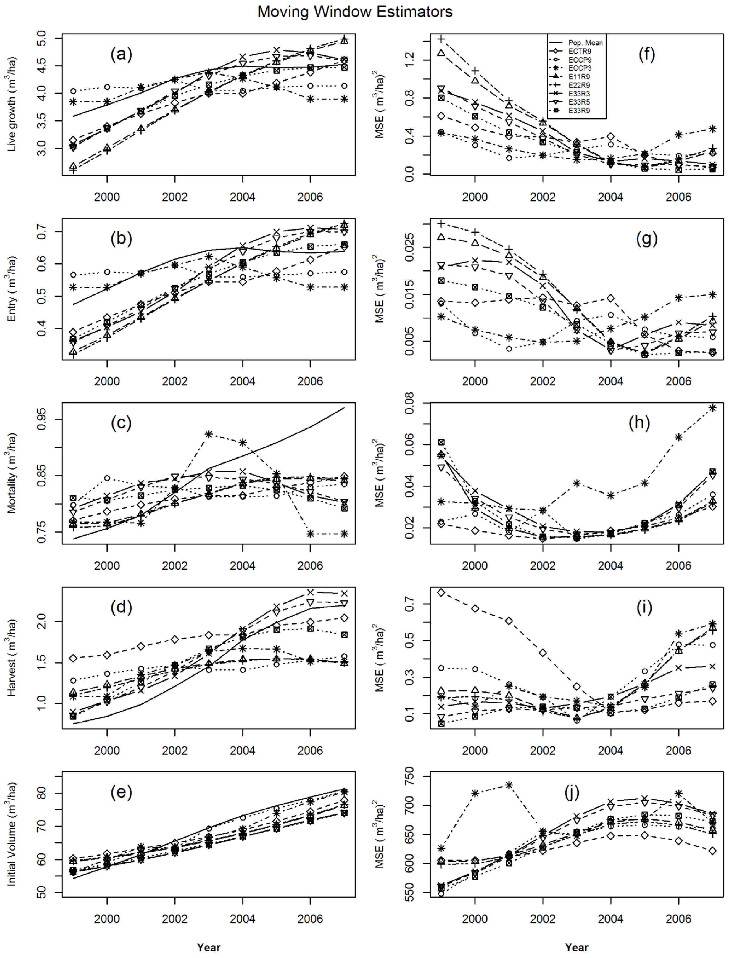
2.3. Moving-Window Mean of Ratios Estimator

Our estimation approach uses the (semi-centralized) moving-window mean of ratios estimator (MWMOR) in Roesch and Van Deusen [3] and Roesch [6], an estimator that arose from a different perspective than previously-developed estimators. The idea was simple. One stacks the observations on a temporal scale (or a function of the temporal scale) and then slices through the stack (say to create annual segments) to determine what proportion of each observation contributes to the estimate for each year spanned by the observation. For this problem, as in Roesch and Van Deusen [3], we use the general three-dimensional selection model given in Roesch [2] with the exception that time will be re-scaled relative to the proportion of the growing season elapsed within each year. Assign to each observation of variable x labels for plot i and a superscript representing the beginning value and ending value as xib and xie, respectively. Because there are no observations between xib and xie, the distribution of the volume growth between the two observations must be modeled. In Roesch and Van Deusen [3], two simplifying assumptions were made. In the first, it was assumed that the growing season begins and ends on the same dates for each year in the area of interest. In the second, it was assumed that growth for each plot is uniform throughout the growing season. Given these assumptions, we can temporally order each observation by the year of observation plus the proportion (p) of the growing season that has elapsed. We use si to represent the difference in these values to obtain the growing season-adjusted temporal span between the beginning and ending observations. We then allocate the proportion of growth observed over si to the proportion of each year spanned by si, (thereby accounting for the marginal probability of the time dimension). Modeling growth between observations allows us to allocate growth within components to the years the growth occurred. A simple time-adjusted estimator for annual volume growth (within the growth component) is the moving-window mean of ratios estimator (MWMOR) for component C in year t:
C t M = 1 n t i = 1 n t c i , t p i , t
where:
  • n t = the number of plots observing growth in year t;
  • p i , t = the product of portion of year t growing season observed by plot i and the portion of plot i area within the area of interest and;
  • c i , t = the value of component C observed on plot i, assignable to year t.
The general statistical properties of ratio estimators are well known and can be found in very early works, such as Raj [15], Walton and DeMars [16], Cassel et al. [17] and Cochran [18].
In some of the estimators below, we use a trend distributed version of C t M in which c i , t in Equation (2) is replaced by c i , t T . The value of c i , t T is determined by the value of the trend in initial cubic meter volume at year t. A proportion is allocated to each year observed in a plot remeasurement interval, c i , t T = π y x i , where xi is the total value of a change component (such as live growth) observed over an interval of years y = 1 to Y, and π y = v y / j = 1 Y v j , where vj is the sample mean initial volume for year j. Note that we use the variable t to refer to the general year within the population or estimation interval and the variable y to refer to the year within a particular sample plot’s remeasurement interval. Because plots are measured in panels, y selects a panel-specific subset of t. We use this change of variable below, where it is appropriate. The underlying assumption of c i , t T is that the level of a change component during a particular year will be proportional to the standing volume at the beginning of the year. The trend distributed estimators then take the form:
C t T = 1 n t i = 1 n t c i , t T p i , t

2.4. Incorporating Image Change Estimates

Roesch [6] demonstrated the utility of a weighting method that can be used in conjunction with the MWMOR estimators above. We use a variant of that approach here in order to use the remotely-sensed information to better approximate the timing of harvests and the corresponding allocation of the components of change within a remeasurement window.
We simulated the incorporation of ICE observations from remotely-sensed images every two years under three different assumptions of reliability. In Assumption 1 (A1), a clearcut, defined as the harvest of at least 95% of the cubic-meter volume, is successfully identified in the image 95% of the time, and there are no false positives. Under this assumption, when a clearcut is identified, it is known to have occurred since the last plot visit, but may have been missed during intervening ICE observations. Under Assumption 2 (A2), all clearcut harvests are correctly identified 100% of the time and assigned to the correct year. Again, there are no false positives. Assumption 3 (A3) reflects the highest level of reliability in which every harvest (whether a partial harvest or a full harvest) is identified and assigned to the correct year; we can estimate the proportion harvested to within ±5% (truncated at 0% and 100%), and there are no false positives.
Under all three of these reliability assumptions, ICE data collected every two years will be in sync with about half of the plot observations collected under the panel design and out of sync with the other half. That is, one panel or 1/10 of the plots is observed every year, and the ICE observations are made every year. For half of the plots, the first ICE observation made after the plot observation will be in one year, and for the other half of the plots, the first ICE observation after the plot observation will be in two years.
There are a number of different approaches that could be taken to determine the weights used to allocate the change components to the intervening years, depending on the analyst’s prior knowledge with respect to the reliability of the ICE data and the availability of reasonable growth models. For instance, by the clearcut definition above, up to 5% of the cubic-meter volume could remain on live trees, and new trees could develop and grow subsequent to the harvest and prior to the next sample plot observation. For partial harvests, the possibility for subsequent growth is much higher. In large countries with a very diverse range of species and forest types, there are often not reasonable growth models available for many of those types. Additionally, there will usually be unobserved growth on trees that die or are harvested during the observation interval. In the case of a clearcut, this unobserved growth occurred on the prior stand, so it is reasonable to assume that it will usually far outweigh the observed growth, because growth is observed only on trees present at the next plot observation. Therefore, under Assumptions 1 and 2, we simplify the annual allocation problem by assuming that all observed growth occurred before the ICE clearcut observation. Under Assumption 3, for all harvests, we use an allocation that separates pre-harvest and post-harvest change based on an estimate of the proportion of volume harvested.

2.4.1. Estimation under A1

Under Assumption A1, when a clearcut is identified, it is known to have occurred since the last plot observation, but may have been missed during intervening ICE observations. To establish weights, we could either use an estimate of the probability of having missed the clearcut at previous ICE observations or we could assume that the probability is unknown. Because A1 is intended to be our worst case assumption in the simulation, we assumed that this probability was unknown. The allocation of partial harvest volumes is unaffected by ICE observations under this assumption.
We define y i , I as the number of years of the first ICE observation of clearcut for plot i since the previous plot measurement. Although it would be a rare event, we also define y i , I I y i , I I + 2 as the year of the second ICE observation of clearcut for plot i during the remeasurement interval, in order to estimate the weight for harvest. Additionally, when there are two ICE-identified clearcuts on plot i, we define ri,I as the proportion of total clearcut volume in the first clearcut and ri,II = 1 − ri,I as the proportion of total clearcut volume in the second clearcut.
π i , y T h A 1 = { π y if no ICE-identified clearcut y i , I 1 if one ICE-identified clearcut and  y y i , I r i , I if ICE is out-of-sync with two identified clearcuts and  y = y i , I . 5 r i , I if ICE is in-sync with two identified clearcuts and  y = y i , I 1 . 5 r i , I if ICE is in-sync with two identified clearcuts and  y = y i , I . 5 r i , I I if two ICE-identified clearcuts and  y = y i , I I 1 . 5 r i , I I if two ICE-identified clearcuts and  y = y i , I I 0 otherwise
The proportion ri,I would have to be estimated. An estimate might be obtained from the ICE data, but it is not directly available from the sample plot data. Under A1, we do not assume that we can confidently estimate ri,I from the images, so we set it equal to 0.5. The allocation for the harvest component on plot i for year t under A1 is:
h i , t T h A 1 = π i , y T h A 1 h i
where hi is the observation of cubic meter harvested volume on plot i during the remeasurement interval. The estimator for the harvest component for year t under A1 is:
C t h A 1 = 1 n t i = 1 n t h i , t T h A 1 p i , t
For the other components of change (live growth, entry and mortality), the allocation to each year between plot observation and ICE clearcut call:
π i , y T o A 1 = { π y if no ICE-identified clearcut                             y i , I 1 if one ICE-identified clearcut and  y y i , I     0       if no ICE-identified clearcut and  y > y i , I     π y     if two or more ICE-identified clearcuts     
The allocation for the other components of change on plot i for year t under A1 is represented as o i , t T o A 1 = π i , y T o A 1 o i , where oi is the observation of a specific component o for plot i during the interval. The estimator for the other components of change for year t under A1 is:
C t o A 1 = 1 n t i = 1 n t o i , t T o A 1 p i , t

2.4.2. Estimation under A2

Under Assumption 2 (A2), we know if a clear-cut has occurred within the past two years, and we can assign it to the correct year. As under A1, the allocation of partial harvest volumes is unaffected by ICE observations. The weight for the harvest component is defined as:
π i , y T h A 2 = { π y if no ICE-identified clearcut 1 if one ICE-identified clearcut and  y = y i , I r i , I if two ICE-identified clearcuts and  y = y i , I r i , I I if two ICE-identified clearcuts and  y = y i , I I 0 otherwise
As we mentioned above, the proportion ri,I would have to be estimated, and it is not directly available from the sample plot data. However, by definition, a clearcut consists of the harvest of 95% of the volume present during the year of harvest, so ri,I could be approximately estimated by:
r ^ i , I = v I v I + v I I
where v I is the sample mean initial volume for year for the year of the first ICE-identified clearcut and v I I is the sample mean initial volume for the year of the second ICE-identified clearcut. An estimator for r i , I I would then be r ^ i , I I = 1 r ^ i , I .
The allocation for the harvest component on plot i for year t under A2 is:
h i , t T h A 2 = π i , y T h A 2 h i
This leads to the estimator for the harvest component for year t under A2:
C t h A 2 = 1 n t i = 1 n t h i , t T h A 2 p i , t
For the other components of change, if there were a single clearcut, we assign all observed growth to the years prior to the ICE clearcut observation, but otherwise, we use proportional allocation as described above. We define the value of the trend by a proportion that is allocated to each year y in an interval beginning with the year of the sample plot observation for plot i and ending with the year of the first ICE observation of clearcut ( y i , I ):
π i , y I = v y j = 1 y I v j
Then, the weight for the other components is:
π i , y T o A 2 = { π y if no ICE-identified clearcut π i , y I if one ICE-identified clearcut and  y y i , I π y if two ICE-identified clearcuts 0 otherwise
The allocation for the other components on plot i for year t under A2 is then:
o i , t T o A 2 = π i , y T o A 2 o i
The estimator for the other components of change for year t under A2 is:
C t o A 2 = 1 n t i = 1 n t o i , t T o A 2 p i , t

2.4.3. Estimation under A3

Under Assumption 3 (A3), we know if any harvest has occurred within the past two years and which year the harvest occurred. We will assume that proportional growth occurred before and after ICE harvest observations and that we can estimate the proportion harvested to within ±5% (truncated at 0% and 100%). Let π i , y h be the ICE-estimated proportion of volume harvested in year y on plot i. Then, the weight for the harvest component under A3 is:
π i , y T h A 3 = { π y if no ICE-identified harvest in observation interval π i , y h if ICE-identified harvest in year  y 0 otherwise
The harvest allocation on plot i for year t under A3 is:
h i , t T h A 3 = π i , y T h A 3 h i
This results in the estimator for the harvest component for year t under A3:
C t h A 3 = 1 n t i = 1 n t h i , t T h A 3 p i , t
To determine the allocation for the other components of change, let π i , F h be the first (in year F, yF) ICE-estimated proportion of volume harvested on plot i and π i , S h be the second (in year S, yS) ICE-estimated harvest proportion on plot i. We set π i , F h = 0 if there is not an ICE-identified harvest during the interval, and we set π i , S h = 0 if there are not two ICE-identified harvests during the interval. The proportion remaining following the first harvest on plot i is π i , F R = 1 π i , F h . Likewise, the proportion remaining following the second harvest on plot i is π i , S R = 1 π i , S h . We calculate the annual allocation in three parts:
a y = { ( π i , F h π y ) / j = 1 y F π j if one or two ICE-identified harvests and  y y F 0 otherwise                                                                   
b y = { ( π i , F R π i , S h π y ) / j = 1 y S π j if two ICE-identified harvests and  y y S 0 otherwise                                                                
and:
c y = ( π i , F R π i , S R π y )
We then sum the parts to obtain the annual proportion:
π i , y T o A 3 = a y + b y + c y
The allocation under A3 then becomes:
o i , t T h A 3 = π i , y T o A 3 o i
Finally, the estimator for each of the other components under A3 is:
C t o A 3 = 1 n t i = 1 n t o i , t T o A 3 p i , t

2.5. Compatibility and the Estimation of Initial Volume

In the previous subsections, we have described the estimators for the components of change. A complete estimation system also requires an estimator for initial volume. If the estimation system is also required to be compatible, as defined in Section 1, then some means of ensuring compatibility is required. We caution the reader that to ensure compatibility in an equation system is to enforce a constraint, and every constraint leads to a sub-optimization of one or more of the system’s estimators.
The plot sample provides single-panel direct annual estimates of standing volume, while we desire estimates of standing volume at the beginning of the year or prior to the growing season. We assume that each panel’s estimate of mean standing volume is a mid-year estimate, because sample plots are measured throughout the year. There are a number of approaches that could be taken, but the simplest approach would be to take the mean of successive panel means to obtain the initial annual estimates. For i = 1998 to 2006:
Y ^ i + 1 P = .5 ( v ¯ i P + v ¯ i + 1 P )
where v ¯ j P is the (assumed mid-season) standing volume estimate for panel j. We denote this series of estimates as Y ^ P .
Alternatively, because Y ^ P does not ensure compatibility of the estimation system, we can use recursive estimation to estimate initial annual volume. That is, we can start with an initial volume estimate for a particular year and successively apply the annual estimators of the components of change to obtain successive estimates of initial annual volume. In the simulation, we started with the initial volume estimate for the year 2003, ( Y ^ 2003 R = Y ^ 2003 P ), which is in the center of the estimation interval. To obtain the recursive series of estimates ( Y ^ R ) for 1999 to 2007, we used the algorithm:
For i = 2003 to 2006:
Y ^ i + 1 R = Y ^ i R + L ^ i + E ^ i M ^ i H ^ i
For earlier years we use, for i = 2003 to 2000:
Y ^ i 1 R = Y ^ i R L ^ i 1 E ^ i 1 + M ^ i 1 + H ^ i 1

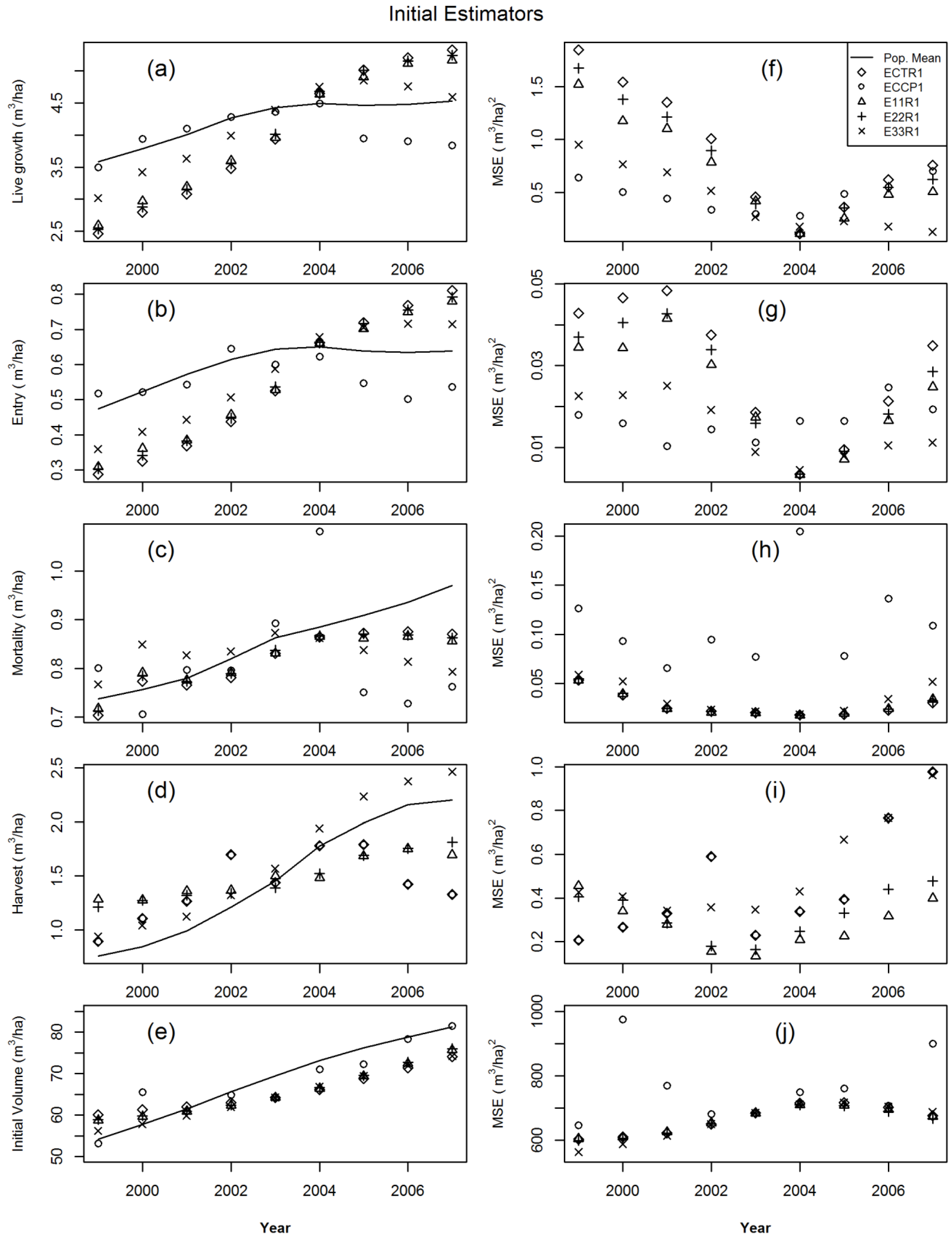
2.6. Estimation Systems

The estimators described in the preceding sections can be combined in various ways to define an estimation system. Furthermore, variance reduction can be achieved in the estimators by combining successive estimates with a moving window estimator. For any initial estimator for time t ( ε t ), a moving window estimator of size s (s is an odd positive integer) is:
ε i s = i = t ( ( s 1 ) / 2 ) t + ( ( s 1 ) / 2 ) ε i
The estimation systems that we tested in the simulations will be easiest to follow if we define an estimation system nomenclature. In the nomenclature, the character “E” is followed by a 4-character code (e.g. E1234). The 1st character is for harvest; the 2nd character is for the other growth components; the 3rd character is for initial volume; and the 4th character is for the moving window size:
  • ECCP1 = CM for all change components and Y ^ P for initial annual volume,
  • ECTR1 = CM for harvest, CT for the other change components, Y ^ R for annual volume,
  • E11R1 = ChA1 for harvest, CoA1 for the other change components, Y ^ R for annual volume,
  • E22R1 = ChA2 for harvest, CoA2 for the other change components, Y ^ R for annual volume,
  • E33R1 = ChA3 for harvest, CoA3 for the other change components, Y ^ R for annual volume,
  • ECCP3 = 3-year moving window on ECCP1,
  • ECCP9 = 9-year moving window on ECCP1,
  • ECTR9 = 9-year moving window on ECTR1,
  • E11R9 = 9-year moving window on E11R1,
  • E22R9 = 9-year moving window on E22R1,
  • E33R3 = 3-year moving window on E33R1,
  • E33R5 = 5-year moving window on E33R1 and,
  • E33R9 = 9-year moving window on E33R1.

2.7. Estimator Evaluation

For each iterate, for each year, we calculated the empirical bias (EB) and the empirical mean squared error (MSE), over the 1000 iterations, between each estimator and the true population values under each of the four error structures.
That is:
E B P E S = 1 1000 i = 1 1000 ( x ^ P E S i X P )
where x ^ P E S i is the sample estimate of any variable, X, in population P for estimator E, under error structure S for iterate i. Likewise:
M S E P E S = 1 1000 i = 1 1000 ( x ^ P E S i X P ) 2
Here, we use the empirical mean squared error as the overriding criterion for judging the effectiveness of the external information while being cognizant of any introduced bias. Estimator robustness was tested in a simulation by sampling the population under four different assumptions of sampling error structure for the plot data and three different assumptions of the accuracy of the remotely-sensed data. Each simulation consisted of 1000 iterations of 1000 plots each (without replacement) from the population.

3. Results

Figure 1 gives the empirical means of the components of change and initial annual volume plotted with the true population mean on the left-hand side and mean squared errors on the right-hand side of the initial annual estimators (ECTR1, ECCP1, E11R1, E22R1 and E33R1) for estimation years 1999 through 2007. The results are given subsequent to 1000 iterations of 1000 samples each under Sample Error Structure 1. The corresponding results for these components of change for Error Structures 2 through 4 are available from the first author upon request. They are not given here, in the interest of brevity, because they are very similar to the results for Error Structure 1.
The differences between each annual mean and the true population mean on the left-hand side of Figure 1 is the empirical bias (EBPES) described above, for each estimator. These estimation years are shown because they are the years that are the center of at least 1 observation window (or panel), for a sample drawn under this design and sample error structure from a population spanning 1995 to 2012. From Figure 1, it is obvious that the ICE observations usually served to lower the bias for estimates of annual harvest. This usually, though not exclusively, also resulted in lowered empirical mean squared errors for the annual harvest estimates. Figure 1 also shows that the general trend model had a positive effect on mortality estimates, while using the trend model for entry and live growth showed mixed results.
This work was predicated on the assumption that the improvement in harvest estimates obtainable through the use of the ICE observations will also result in better estimates of annual volume. The bottom row of Figure 1 investigates that assumption. Of the single-panel estimators for initial (1 January) annual volume in the bottom row of Figure 1, ECCP1 can be seen to be the most variable.
Figure 1. The empirical means of the initial annual estimators (ECTR1, ECCP1, E11R1, E22R1 and E33R1) plotted with the true population mean for (a) live growth; (b) entry; (c) mortality; (d) harvest; and (e) initial volume; and the corresponding mean squared errors for (f) live growth; (g) entry; (h) mortality; (i) harvest and (j) initial volume, from the simulation of 1000 iterations of 1000 samples each under Sample Error Structure 1.
Forests 06 02897 g001
Figure 2 gives the empirical means plotted with the true population mean on the left-hand side and mean squared errors on the right-hand side of the moving-window annual estimators (ECTR9, ECCP9, ECCP3, E11R9, E22R9, E33R3, E33R5 and E33R9) over 1000 iterations of 1000 samples, each under Sample Error Structure 1. As expected, the moving window estimators “smooth” the mean annual estimates and usually serve to lower the annual empirical mean squared errors for the components relative to the corresponding results in Figure 1. The bottom row of Figure 2 gives the results for the moving window annual estimators of annual volume. As in Figure 1, this row shows some advantage to combining panels. For instance, the MSEs are slightly less variable in the early years for ECCP3, relative to the results for ECCP1 in the top row of the figure. ECCP9 shows an even further reduction in MSE for most years, relative to ECCP3.
Figure 2. The empirical means of the moving window annual estimators (ECTR9, ECCP9, ECCP3, E11R9, E22R9, E33R3, E33R5 and E33R9) plotted with the true population mean for (a) live growth; (b) entry; (c) mortality; (d) harvest; and (e) initial volume; and the corresponding mean squared errors for (f) live growth; (g) entry; (h) mortality; (i) harvest and (j) initial volume, from the simulation of 1000 iterations of 1000 samples each under Sample Error Structure 1.
Forests 06 02897 g002
Although we are only showing the results for Error Structure 1, we note that the ranking of the mean for each annual estimator remained constant through the four error structures, although the position of each annual group of estimators did change slightly with error structure.

4. Discussion and Conclusions

Roesch [6] explored some special problems that arise in estimation of the components of change when the temporal scale of the population estimand of interest is finer than the scale of observation under both biased and unbiased sampling error structures. Here, we go further and attempt to ameliorate the effects of an unplanned increase in the temporal interval between observations. In the example simulations, the temporal scale of observation was increased from five to 10 years, while the temporal dimension of the population of interest and the estimands of interest remained fixed at one year.
As discussed in Roesch [6], by definition, the MW estimator is non-centralized and uses the information for all plots whose intervals span a particular year. This can allow the use of more data in the years at the extremes of a period of interest, but will lead to a reduced ability to detect trend changes. This effect is intensified for longer cycle lengths. That is, when the design observes five-year windows, an estimate of average annual change “smooths” the actual annual change, and the estimators, while drawing strength from overlapping panels, provide further smoothing. Both of these effects are substantially increased when the cycle length is changed to 10 years. The simulations showed the variance/bias trade-off encountered when the moving-window mean of ratios estimator was used in the extremity years of observation. Although the MWMOR estimator is sometimes biased in the presence of the trend in the extremity years, the empirical mean-squared error was often much lower when the extraneous information was used. These simulations have accentuated the difficulty that exists when attempting to compensate for an inadequately-informed sample. Large observation intervals frustrate the estimation of even the simplest of trends. We investigated the estimator performance of compatible annual estimators of the components of change during years spanned by at least half of the full set of plot observations, without attempting to address the additional problem arising from the known loss of adequate information in the extreme years of the monitoring effort, which resulted from the lengthened cycles. Never-the-less, we have shown that highly-informative auxiliary observations with shorter observation intervals (as was available under ICE Assumption 3) can contribute to significant improvement in estimation.
Auxiliary information, such as simulated under ICE, may arise from several remote sensing efforts. For example, the National Agriculture Imagery Program (NAIP) collects fine-scale imagery across the United States on a two- to three-year rotating schedule. The manual interpretation of these data for land use, land cover and change information would provide auxiliary observations similar to the ICE scenarios presented in these analyses. Data from other remote sensing efforts may also be appropriate. For example, Li et al. [19] used a time series of Landsat TM imagery to classify changes in forest vegetation and the year that change occurred. Model output arising from Li’s et al. [19] approach could also be informative in our application if modeling error in the classification is in line with the ICE scenarios.
Although our focus in this research was on estimating components of change, ICE-type information, such as described by Webb et al. [20], could aid in estimating several other parameters of interest. For example, forestland provides a suite of ecosystem services, and changes in the use of the forestland base influence the availability of those services (Coulston et al. [21]). Van Deusen and Roesch [4] and Coulston et al. [21] provide temporally-specific approaches to estimate changes in the use of forestland, based on remeasured plot data alone. Including auxiliary data on land use and/or land cover change may improve the precision of land change estimates. However, further development and testing of appropriate temporally-specific estimators is required to take full advantage of the auxiliary information. Temporally-specific estimators serve to increase the relevance and timeliness of NFI data. Using temporally-dense remote sensing data to assist in the estimation may provide an opportunity for national forest inventories whether or not fiscal climates are uncertain. However, the inclusion of auxiliary data that is more temporally dense than the plot data has the potential to provide improvement only if time is specifically accounted for in the estimation process, as is the case here.

Acknowledgments

The authors were funded by their respective institutions. The seed data for the simulations were collected by the United States Department of Agriculture’s Forest Service, Forest Inventory and Analysis Program.

Author Contributions

Francis A. Roesch, John W. Coulston and Paul C. Van Deusen identified the need for the study and discussed potential approaches. Francis A. Roesch designed and constructed the test population and the sampling simulations and wrote the first draft. John W. Coulston, Paul C. Van Deusen and Rafał Podlaski commented on the first draft and contributed to the revision of the manuscript.

Conflicts of Interest

The authors declare no conflict of interest.

References

  1. Tomppo, E.; Schadauer, K. Harmonization of national forest inventories in Europe: Advances under COST Action E43. For. Sci. 2012, 58, 191–200. [Google Scholar] [CrossRef]
  2. Roesch, F.A. An alternative view of continuous forest inventories. For. Sci. 2008, 54, 455–464. [Google Scholar]
  3. Roesch, F.A.; Van Deusen, P.C. Time as a Dimension of the Sample Design in National-Scale Forest Inventories. For. Sci. 2013, 59, 610–622. [Google Scholar] [CrossRef]
  4. Van Deusen, P.C.; Roesch, F.A. Estimating forest conversion rates with annual forest inventory data. Can. J. For. Res. 2009, 39, 1993–1996. [Google Scholar] [CrossRef]
  5. Roesch, F.A.; Van Deusen, P.C. Monitoring forest/non-forest land use conversion rates with annual inventory data. For. Int. J. For. Res. 2012, 85, 391–398. [Google Scholar] [CrossRef]
  6. Roesch, F.A. Toward robust estimation of the components of forest population change. For. Sci. 2014, 60, 1029–1049. [Google Scholar] [CrossRef]
  7. Eriksson, M. Compatible and time-additive change component estimators for horizontal-point-sampled data. For. Sci. 1995, 41, 796–822. [Google Scholar]
  8. Roesch, F.A. The components of change for an annual forest inventory design. For. Sci. 2007, 53, 406–413. [Google Scholar]
  9. Bechtold, W.A.; Patterson, P.L. The Enhanced Forest Inventory and Analysis Program-national Sampling Design and Estimation Procedures; U.S. Department of Agriculture Forest Service Southern Research Station: Asheville, NC, USA, 2005; Available online: http://www.srs.fs.fed.us/pubs/20371 (accessed on 16 July 2015).
  10. McCollum, J.M. Honeycombing the icosahedron and icosahedroning the sphere. In Proceedings of the second annual Forest Inventory and Analysis Symposium, Salt Lake City, UT, USA, 17–18 October 2000; Reams, G.A., McRoberts, R.E., Van Deusen, P.C., Eds.; USDA Forest Service Southern Research Station: Asheville, NC, USA, 2001; pp. 25–31. Available online: http://www.srs.fs.fed.us/pubs/4527 (accessed on 16 July 2015). [Google Scholar]
  11. Van Deusen, P.C. Alternatives to the Moving Average. In Proceedings of the second annual Forest Inventory and Analysis Symposium, Salt Lake City, UT, USA, 17–18 October 2000; Reams, G.A., McRoberts, R.E., Van Deusen, P.C., Eds.; USDA Forest Service Southern Research Station: Asheville, NC, USA, 2001; pp. 90–93. Available online: http://www.srs.fs.fed.us/pubs/4537 (accessed on 16 July 2015). [Google Scholar]
  12. Roesch, F.A.; Steinman, J.R.; Thompson, M.T. Annual Forest Inventory Estimates Based on the Moving Average. In Proceedings of the third annual Forest Inventory and Analysis Symposium, Traverse City, MI, USA, 17–19 October 2001; McRoberts, R.E., Reams, G.A., Van Deusen, P.C., Moser, J.W., Eds.; USDA Forest Service North Central Research Station: St. Paul, MN, USA, 2003; pp. 21–30. Available online: http://www.nrs.fs.fed.us/pubs/gtr/gtr_nc230.pdf#page=27 (accessed on 16 July 2015). [Google Scholar]
  13. Van Deusen, P.C. Issues Related to Panel Creep. In Proceedings of the third annual Forest Inventory and Analysis Symposium, Traverse City, MI, USA, 17–19 October 2001; McRoberts, R.E., Reams, G.A., Van Deusen, P.C., Moser, J.W., Eds.; USDA Forest Service North Central Research Station: St. Paul, MN, USA, 2003; pp. 31–35. Available online: http://www.nrs.fs.fed.us/pubs/gtr/gtr_nc230.pdf#page=37 (accessed on 16 July 2015). [Google Scholar]
  14. Westfall, J.A.; Frieswyk, T.; Griffith, D.M. Implementing the Measurement Interval Midpoint Method for Change Estimation. In Proceedings of the Eighth Annual Forest Inventory and Analysis Symposium, 16–19 October 2006; Monterey, C.A., McRoberts, R.E., Reams, G.A., Van Deusen, P.C., Williams, W.H., Eds.; USDA Forest Service: Washington, DC, USA, 2009; pp. 231–236. Available online: http://www.nrs.fs.fed.us/pubs/gtr/gtr_wo079/gtr_wo079_231.pdf (accessed on 16 July 2015). [Google Scholar]
  15. Raj, D. Sampling Theory; McGraw-Hill: New York, NY, USA, 1968. [Google Scholar]
  16. Walton, G.S.; DeMars, C.J. Empirical methods in the evaluation of estimators. In USDA Forest Service Research Paper NE-272; USDA Forest Service; Northeastern Forest Experiment Station: Upper Darby, PA, USA, 1973; Available online: http://www.fs.fed.us/ne/newtown_square/publications/research_papers/pdfs/scanned/OCR/ne_rp272.pdf (accessed on 16 July 2015).
  17. Cassel, C.M.; Särndal, C.E.; Wretman, J.H. Foundations of Inference in Survey Sampling; John Wiley & Sons: New York, NY, USA, 1977. [Google Scholar]
  18. Cochran, W.G. Sampling Techniques, 3rd ed.; John Wiley & Sons: New York, NY, USA, 1977. [Google Scholar]
  19. Li, M.; Huang, C.; Zhu, Z.; Shi, H.; Lu, H.; Peng, S. Assessing rates of forest change and fragmentation in Alabama, USA, using the vegetation change tracker model. For. Ecol. Manag. 2009, 257, 1480–1488. [Google Scholar] [CrossRef]
  20. Webb, J.; Brewer, C.K.; Daniels, N.; Maderia, C.; Hamilton, R.; Finco, M.; Megown, K.; Lister, A.J. Image-based change estimation for land cover and land use monitoring. In Moving from Status to Trends: Forest Inventory and Analysis (FIA) Symposium 2012; Morin, R.S., Liknes, G.C., Eds.; USDA Forest Service Northern Research Station: Newtown Square, PA, USA, 2012; pp. 46–53. Available online: http://www.nrs.fs.fed.us/pubs/gtr/gtr-nrs-p-105papers/08webb-p-105.pdf (accessed on 16 July 2015).
  21. Coulston, J.W.; Reams, G.A.; Wear, D.N.; Brewer, C.K. An analysis of forest land use, forest land cover and change at policy-relevant scales. Forestry 2014, 87, 267–276. [Google Scholar] [CrossRef]

