An Area-Based Matrix Model for Uneven-Aged Forests

Abstract

In this paper a new concept for modeling uneven-aged forests (UEAF) is presented. The term UEAF in this article encloses all forests that deviate from the even-aged structure. The matrix model is area-based, in that the forest under study is described by a distribution of areas over fixed state-spaces spanned by stem number and volume per hectare classes. Dynamics is introduced as transitions of areas inside the state-space during the simulation. Harvesting activities and the occurrence of calamities are explicitly handled. The model is designed to be suitable for large-scale analyses. The concept was tested in an application to Austrian National Forest Inventory (NFI) data. Results shown, including a comparison to older inventory data, indicate that it is worth further elaborating on the concept and the model. The work will be continued and in the next step the model concept will be applied in several other countries.

1. Introduction

When aiming for a forest analysis on European level, it is essential to handle the even-aged forests common in Northern Europe as well as the multistoried, uneven-aged forest of Central and Southern Europe. Most large-scale forest models meet challenges when trying to model the dynamics of uneven-aged forests. On single-stand-level numerous, normally diameter class or individual tree equation based, models have been developed and applied [1,2,3] (Chapter 15). However, it has shown to be difficult to scale up these models to the forest-level.

Multiple definitions for uneven-aged forests exist. In some cases the naming has been deduced from the management applied; if it is selective and a continuous forest cover is maintained, this naturally leads to a forest having differently aged trees (e.g., [3]). Sometimes through the diameter distribution range; for example, if the range is more than three consecutive 4–5 cm diameter classes, stands are classified as uneven-aged [4,5]. Hanewinkel et al. [6] even introduce an index of “closeness to a J-shaped distribution” because the diameter distribution of an uneven-aged forest is typically assumed to be reverse-J shaped. All the definitions agree that in uneven-aged forests the sizes of trees vary and, indeed, tree size is a more relevant characteristic of a forest stand than age [4,7,8].

There are various terms used in the literature when referring to uneven-aged forests, for example, mixed, irregular, heterogeneous, continuous cover, multi-cohort and all-aged or all-sized forests. The multitude of terms and definitions suggests that applying a uniform definition, valid in all circumstances for all different types of uneven-aged forests, is not at all trivial. However, in order to avoid additional confusion, we will in this paper use the term “uneven-aged forest” (UEAF), denoting thereby all forests that deviate from the even-aged structure. We wish to stress that it is a heterogeneous group of forests, including a rather broad range of stand structures in which feasible/reasonable management practices and activities vary.

There are basically two approaches for modeling the dynamics of a forest or a forest stand. The most common is to describe the forest as a fixed set of units, trees or stands, each unit having a number of attributes, such as species, diameter, height or age. Dynamics are then expressed as changes of the attributes. An alternative is to define a set of fixed states and then let some entity (areas, trees) move between the states to illustrate dynamics. The latter approach is employed in a number of applications, often referred to as matrix models [9,10,11,12].

The most common type of matrix models for UEAF stands is based on defining the set of states by diameter classes, using the number of trees falling into the different classes as the description of the state of the stands i.e., diameter distribution. Dynamics is then introduced by transitions of trees between the diameter classes during a fixed time period. These models have been proven to depict the dynamics of single forest stands reasonably well. They were applied on uneven-aged stands already in the 1970s [13]. Throughout the years, several studies were conducted to improve the model and estimation procedures e.g., [9,14,15,16,17,18,19,20,21,22]. However, these models encounter problems when applied to a forest that consists of many different stands.

A recent review article notes that matrix models have already been used in almost all possible situations related to forestry [23], including large-scale mapping of timber, biomass resources assuming constant climate [24,25], and under climate change scenarios [26]. However, the authors of the review [23] understand by “Matrix models” only the tree-based diameter class models and do not cover the use of area-based matrix models for large-scale applications. Yet, area-based matrix models have been highly prominent on the European large-scale forest modeling arena [12,27,28].

To appreciate the difference between diameter class and area-based matrix models, it is essential to separate between tree-based and area-based and between stand-level and forest-level models. While trees are moving between fixed states, diameter classes, defined for an individual stand in the tree-based models, in the area-based models, areas—possibly represented by plots—are transiting in a common state-space. The area-based matrix models used in, for example, Sallnäs [11], Nilsson, Sallnäs and Duinker [27], Nabuurs et al. [28] and Schelhaas et al. [12] are structurally similar, although based on different data sets. These studies all are aiming at national or European scale analyses with a focus on even-aged forests.

To date, the most commonly applied area-class matrix models are based on a state-space defined in terms of volume and age (e.g., [12,27,28,29]). Age is a crucial variable in modeling the dynamics of even-aged forests, but is non-existent at plot and stand levels when UEAF is concerned. With the age variable excluded, the information on volume, especially in the UEAF case, is insufficient for reasonable predictions of its dynamics. Thus, another variable is needed in addition to volume for the area-based approach to work for UEAF.

We applied the area-based matrix concept to UEAFs by defining the state-space by volume and number of stems per unit area. We conjectured that stem number, when coupled with volume, would bring a substantial amount of information as to the growth pattern and allow for a reasonable model of UEAF while preserving the inherent advantages of the area-class matrix model.

In this paper we describe an area-based matrix modeling approach for UEA forests and discuss the potential for its application in large-scale analyses. In addition, we show the first application of the developed method to real National Forest Inventory (NFI) data from Austria.

2. Material and Methods

2.1. Data

The Austrian NFI [30,31] has had a permanent sampling plot grid for several decades, allowing analyses of forest development over an extended period of time. The sampling grid has a regular, square shape with a side length of 3.89 km. At each point in the grid there is a cluster of four sampling plots where an angle count sample is taken. This means that there are about 22,000 plots all over Austria, of which 9,563 provided forest data in the inventory period 7 (2007–2009). The number changes slightly every period, because non-forest may change into forest and vice versa.

For this study, data from the periods 6 (2000–2002) and 7 (2007–2009) are used in estimation of the transition and activity probabilities. In addition, data from the older inventory period 3 (1981–1985) is employed as an alternative starting point for simulations in order to compare simulated figures against the data from the later inventories.

All data sets comprise the following variables:

• stem number per hectare;
• growing stock in m³ per hectare;
• dominant species;
• altitude above sea level in m; and
• ownership.

The plots are sampled with an angle gauge of basal area factor of 4. This means that each tree, which is selected by the angle gauge and measured at the plot, represents 4 m² of basal area per hectare. Since NFI data was used, all necessary diameter measurements were available. Thus, the basal area of every sample tree is known and an estimate of the number of stems per hectare is easily calculated by dividing 4 m² by the basal area of the sample tree and then summing up over all trees in the sample plot:

$$n= {{\displaystyle \sum }}_i\frac{4}{b_i}$$

(1)

where b_i is the basal area in m² of the ith tree in the plot.

The growing stock is estimated through individual species-specific tree volume models. The single tree volumes on the sample plot are converted into per hectare values and summed up, which gives the estimate of growing stock.

Austria is a country with a large variation in elevation. Therefore the altitude has an impact on the growth potential of forests. Three altitude classes were defined. These classes are below 900 m altitude, between 900 m and 1200 m, and above 1200 m. The class limits were chosen to achieve a relatively equal distribution of the data among the classes while also taking into account the altitudes where changes in the vegetation are noticeable.

The dominant species consists of three classes: Norway spruce (Picea abies), other conifers and broadleaved trees. It was set according to the crown cover, which is assessed in tenths of the plot. The plot had to reach at least eight-tenths of the total cover in one category to be assigned to one of the classes. All other plots were removed from the data set, as well as plots with less than 30% crown cover. Even though eight-tenths sounds like a strict requirement, only a small share was removed from the dataset due to its mixed species structure.

The owner groups are separated into four different classes according to owner type and size of the forest holding. The classes are privately owned forests below 200 ha, between 200 ha and 1000 ha, above 1000 ha, and forest owned by the state of Austria. This was done to open up for differentiating management between owner groups and to capture some of the differences in forest structure due to different historical management, which are not captured by other variables in the model.

For our project we used two selections from the datasets:

Only UEAF plots on which a dominant species could be defined (from inventories 6 and 3, separately, to be used as initial states in the simulations)

2

Only UEAF plots on which a dominant species could be defined and where no harvest had taken place between the inventories 6 and 7 to get information about the natural growth without disturbances from harvests

All plots in the reduced datasets were classified according to the state-space and forest type definitions described above (see also

Table A1. The different classes for forests were defined as follows.

(Factor)	(Value)
Altitude:	(m)
class 1	<900
class 2	900–1200
class 3	>1200
Dominant species:
class 1	Norway Spruce
class 2	other conifers
class 3	broadleaved trees
Stem number:	(lower bound, no. ha−1)
class 1	0
class 2	200
class 3	300
class 4	450
class 5	600
class 6	1000
class 7	1500
class 8	2250
class 9	3500
class 10	5000
Volume:	(lower bound, m3 ha−1)
class 1	0
class 2	63
class 3	92
class 4	134
class 5	188
class 6	259
class 7	347
class 8	452
class 9	575
class 10	710
class 11	852
class 12	994
class 13	1124
class 14	1232
Owner:	(owner group or ha)
class 1	<200
class 2	200–1000
class 3	>1000
class 4	Bundesforste AG 1

¹ The federal forestry company.

). Thus, the total forest area in each class (i.e., state-space cell) could be found as each plot represents ca. 400 ha.

2.2. Model

2.2.1. State-Space

The two variables spanning the state-space, volume and stem number, were classified into, respectively, 15 and 10 disjoint classes. For both variables the class width is increasing with larger values. The ultimate classes are unbounded at the upper limits.

In our implementation like in the other, traditional, areal class matrix models different “forest types” have their own state-space. The objective is to stratify the total forest population into smaller and less heterogeneous groups, which would have similar growth patterns and responses to applied management activities and/or for which differing management could be expected. For the forest type classification, variables that have clear impact on the growth pattern or management of the forests in Austrian conditions and that are readily available were chosen. These variables were dominant species, altitude and owner group as described in the previous section.

In the present version of the model we regard the space defined by the volume and stem number dimensions as the dynamic arena in which transitions take place. That means that during simulations the forest areas stay in the same species class. Naturally, the altitude also remains unchanged and the owner group was kept fixed in this application. In other words, none of the factors used for the forest type classification in the beginning is allowed to change during the simulation.

All the forest related variables that are used, either to span the state-space or to classify the forest types, are presented with their definitions in Appendix 1.

2.2.2. Transitions

Given a set of fixed states S, a set of activities κ and the transition probabilities p_ij, the area matrix model is:

$$\{\begin{array}{c}{x}_j^{t+1}={\displaystyle \sum }_{i,k}{x}_i^t\cdot p_{ij}\left(k^t\right)\cdot a_{ik}^t all i,j \in S, k\in \kappa \\ {{{\displaystyle \sum }}^{\text{}}}_k{a}_{ik}^t=1 all i\in S, k\in \kappa \end{array}$$

(2)

where $x_i^t$ is the area residing in state $i\in \text{S}$ at time t, $a_{ik}^t$ is the fraction of the area in state i that is subject to activity $k\in \kappa$ at time t, and $p_{ij}\left(k^t\right) \in \left[0,1\right]$ is the probability for an area residing in state i at time t to be found in state j at time t + 1 if subjected to activity $k^t$ at time t. The area constraint assures that in each simulation step the whole forest area in the classes of state i is treated and none of it is lost or gained during the simulation.

2.2.3. Activities

We define four activities: No management, final felling, and two different thinning programs: (1) “thLow”, where the area in question is moved down one volume class and two stem number classes, and (2) “thHigh”, where the area is moved down two volume classes and one stem number class. In thLow smaller trees are removed, thus the stem number is changing more than the volume. In thHigh larger trees are removed, and consequently the change in volume is larger. Thinking in terms of forest layers, in the first option mainly trees from the lower height classes are removed, and in the second option mainly from the higher. All four types of activities were discernible in the data despite the fact that “thLow” and final felling might seem to be at odds with the principles of “correct” silviculture for UEAF.

We assumed no direct thinning response in growth: After moving according to the definition of an activity, the area adds to the total area in the given state-space cell and from there “grows” according to “no management” transition probabilities. Hence, the activity specific transition probabilities can be readily deduced once the “no management” probabilities are estimated.

2.3. Estimation of Transition Probabilities

All plots in the dataset No. 2 were classified at two points in time (inventories No. 6 and 7), and the transitions over the volume and stem number classes could be established. These “pair observations” were then fed into the estimation procedure in the EFDM-SC10 software [32]. That procedure is a recursive Bayesian algorithm developed within the EFDM project at the European Commission Joint Research Centre (henceforth JRC) [33]. Essentially, the probabilities are derived from counts of specific transitions of the plots. The probabilities thus estimated refer to a “no management” situation (see the definition of the dataset No. 2 in Chapter 2.1 Data) (see %20ary Data File 1 and %20ary Data File 2 for the estimated transition probabilities and %20ary Data File 3 for the metadata).

2.4. Calamities

Around 10% of the unmanaged plots (dataset No. 2) did move down one or several volume classes between the two inventory times. It could be due to natural mortality, but this loss of volume is a net loss, in the sense that in most cases there is a positive volume increment over a period in time and the gross loss must exceed this. Therefore, we concluded that the loss most probably is due to some calamity. In order to make the simulations more transparent, these transitions were separated and handled in a special manner.

Three new matrices were constructed, averaging by volume and stem number classes the probability of facing a “calamity” and the average loss of volume and stem number. Thus, both the probabilities and the expression of the calamities in terms of changes in volume and stem number classes varied across the state-space.

Combining these three matrices, a calamity transition matrix was generated. Calamities, however, were not handled as an activity, since the probability of a calamity should be equal for all areas in a certain state and thus must be overlapping with activities. Therefore the calamities are assumed to take place in every simulation step before normal activities and growth. In this way it is also possible to vary the occurrence of calamities, through a “calamity coefficient” expressing to what extent the probabilities for calamities estimated from the data should be applied.

2.5. Setting up the Simulations

The model (Equation (2)) described above was applied to model the dynamics of some Austrian forests over a time span of around 100 years. In practice this means that the simulations were run for fifteen 7-year periods, starting from year 2001. An additional simulation was run starting from the year 1983 to compare the simulated development of the forest with the data from the later inventories. This comparison can serve as a test of the adequacy of the transition probabilities estimated from the data of the inventories No. 6 and 7 but only to a certain extent since it is impossible to reflect precisely the forest management that has actually taken place.

Two subsets of forests were chosen for the application based on the data from inventory No. 6 (initial state at year 2001): Norway spruce dominated forests from owner group 1 in altitude classes 1 and 2, respectively. For the additional simulation based on the date from inventory No. 3 (initial state at year 1983) just one subset covering altitude class 1 was used.

For both subsets of the 2001 initial state two different runs were made, changing the harvesting intensity (Table 1). The first one was without any harvests, only including the calamities. The second run included all the available management activities, i.e., thinning and final felling and the calamities. For the 1983 forest only one simulation was run that included the management activities and the calamities.

Since this first simulation aimed at testing the concept, it was decided to use a very simple approach for specifying management in terms of activity probabilities. Average probabilities for the different activities were estimated directly from data, and then applied over the entire state-space with the exception of the two lowest volume classes in which no cuttings occurred.

The cc (calamity coefficient) describes the probability of a calamity. The number denotes the portion of the volume reducing transitions that is assigned to calamities. It was set to 0.42 and 0.50 for the different altitude classes, since these values would generate the same loss in volume in the first step of the simulation as could be deduced directly from the data. The figure of 3% of all areas to be final felled, although counter-intuitive, is derived directly from data. Furthermore, the percentages for the thinning operations correspond to actual data (inventory No. 6).

Table 1. The settings for the activity probabilities in two simulations named “No harvest” and “Harvest” with different harvesting intensities for thinning alternatives “High thinning”(thHigh) and “Low thinning” (thLow), final felling (fF) and calamities (cc).

Simulation	Activity Probability
Run	thHigh (%)	thLow (%)	fF (%)	cc(Altitude Class 1/2)
No harvest	0	0	0	0.42/0.50
Harvest	9	2	3	0.42/0.50

Table 1. The settings for the activity probabilities in two simulations named “No harvest” and “Harvest” with different harvesting intensities for thinning alternatives “High thinning”(thHigh) and “Low thinning” (thLow), final felling (fF) and calamities (cc).

Simulation	Activity Probability
Run	thHigh (%)	thLow (%)	fF (%)	cc(Altitude Class 1/2)
No harvest	0	0	0	0.42/0.50
Harvest	9	2	3	0.42/0.50

3. Results

3.1. Simulations

The results of the simulations based on the 2001 initial state are presented in the Figure 1 and Figure 2. It should be noted that the panel “harv” gives the total harvested volume, i.e., the sum of the panels “thHigh”, “thLow” and “ff”. The panel “cal” gives the volume lost due to calamities, and the panel “incr” gives the total of “harv”, “cal” and the difference of volume between two consecutive points in time. All figures are given in volume/number per ha or per ha and year.

In the simulations without harvests (Figure 1), it is evident that over time the forest state becomes saturated in the sense that the standing stock levels out and the net increase of standing volume approaches 0 because the major part of the gross increment is lost due to calamities. This process develops faster in elevation class 1 than in elevation class 2, resulting in a higher final increment figure for the latter, although the initial increment relation is the opposite.

When harvests are introduced (Figure 2), the increment levels are higher over time, the losses due to calamities are lower and the development of the standing volume levels out at significantly lower levels. Harvested volume increases very slightly in both forest subsets. It is somewhat higher on the elevation class 1, which is logical since the growing stock and increment values are higher there.

In all simulations the average stem number per hectare levels out in the span of 760–840 stems ha⁻¹. It should be noted that the starting values of growing stock and stem numbers are true in the sense of being derived from the inventory data, also the initial harvest amounts are supported by the data through the actual activity probabilities. Thus the plausibility of the simulated outputs to some extent can be judged by the magnitude of their departure from the initial values as well as by their logical consistency.

Figure 1. Development of the Norway spruce forest on elevation class 1 (red line) and 2 (blue dash line) when no harvests are simulated. The calamity coefficients are 0.42 (elevation 1) and 0.5 (elevation 2).

Figure 1. Development of the Norway spruce forest on elevation class 1 (red line) and 2 (blue dash line) when no harvests are simulated. The calamity coefficients are 0.42 (elevation 1) and 0.5 (elevation 2).

3.2. Comparisons with Historical Data and between Simulations

A problem in modeling the development of uneven-aged dominated forests is the scarcity of any basis for validating the model. There is an Austrian model PrognAus [34], which can be applied for any Austrian forest type, but since it is a single-tree based model primarily applicable for stand-level analyses we did not carry out any formal comparisons with our model at this point.

Figure 2. Development of the Norway spruce forest on elevation class 1 (red line) and 2 (blue dash line) when harvests are simulated. The calamity coefficients are 0.42 (elevation 1) and 0.5 (elevation 2). Probabilities for activities are: 9% (high thinning), 2% (low thinning), and 9% (final felling).

Figure 2. Development of the Norway spruce forest on elevation class 1 (red line) and 2 (blue dash line) when harvests are simulated. The calamity coefficients are 0.42 (elevation 1) and 0.5 (elevation 2). Probabilities for activities are: 9% (high thinning), 2% (low thinning), and 9% (final felling).

However, to establish a comparison between some of our simulations and historical records, we used data available from an earlier NFI round, identically classified with the data used in the concept development. We applied the transition and activity probabilities estimated from the other two NFI datasets to this “historical” initial forest state. This older dataset, dated 1983, was at year 2004 after three simulation time steps, while the starting year of the original simulations was 2001. We ran the simulation for full 100 years like in the other cases. In Figure 3, the simulation for elevation class 1 is plotted together with the original simulation based on 2001 initial state.

The two curves converge in all panels after some 10 periods. However, the average volume is significantly higher after three periods in the “1983” run compared to initial situation in the “2001” run, and the average stem number slightly higher. Of course this could be an effect of the harvest level being higher in reality during the period 1983–2004 than reflected by the data from 2001 to 2008. The amount of harvests can vary a lot between single years due to various reasons, from changes in wood prices to storm damages. From numbers obtained from the BFW [35] and in Russ [36] it can be seen that average annual harvests between inventory periods ranged from 4.8 to 6.05 m³ ha⁻¹ and total drain from 5.61 to 7.68 m³ ha⁻¹, which is higher than simulated. There is an annual drain of between 0.3 and 0.92 m³ ha⁻¹ related to calamities. This could be compared to the simulated 2–3 m³ ha⁻¹ of volume loss; the simulated figures are higher, however, it should be remembered that we used only a subset of Austrian forests and that not all volume lost in calamities is necessarily extracted. Also, differentiating between harvests due to calamities and ordinary harvests is very difficult, especially when the inventory takes place several years after the calamity. The higher drain from harvests and the lower drain from calamities partly even each other out.

Figure 3. Development of the Norway spruce forest on elevation class 1 using 1983 (green line) and 2001 (red line) initial states, respectively.

Figure 3. Development of the Norway spruce forest on elevation class 1 using 1983 (green line) and 2001 (red line) initial states, respectively.

Another feature is that in the newer initial state there is a high proportion of forest area in volume and stem number class 1 which we do not find in the older data (Figure 4). This could be an indication of more final felling between the two inventory periods as compared to the time preceding the older inventory.

4. Discussion

It should be underlined that EFDM is not a stand-level model—It is a model for NFI-plots that could be interpreted as a forest-level model. Each NFI plot represents a certain area featuring that specific forest type. However, that area can be, and in most cases is, scattered all over the inventoried area. Most entities with a delineated spatial extent are probably represented by several different plots.

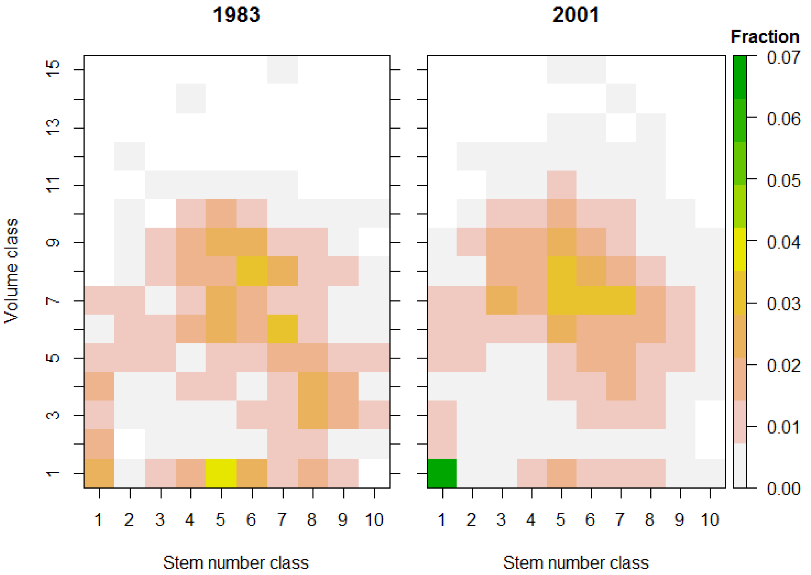
Figure 4. The distributions of areas into the volume and stem number classes for elevation class 1 (Norway spruce) at the initial states “1983” (left) and “2001” (right) illustrated by fractions of the total area.

Figure 4. The distributions of areas into the volume and stem number classes for elevation class 1 (Norway spruce) at the initial states “1983” (left) and “2001” (right) illustrated by fractions of the total area.

It also means that comparing this method to a stand-level diameter class matrix model is difficult, since the basic aims of modeling are different. This model is designed to give estimates for larger areas than a stand-level model. Originally, it was intended for a national level or wider geographical scope analysis. There is a French diameter class model [22] that has been applied in a large-scale analysis, but it is as the authors claim static in a sense that makes it less appropriate for long-term analyses.

The basic assumption used in this study—“the variables standing volume and number of stems can serve as base for modeling the development of a forest area”—can and should be put under question. Of course, one combination of volume and stem number could represent very different forest structures. To some extent this is related to how many “layers” there are in the area. If we regard different forest structures as a continuum, with a perfectly even-aged structure as one extreme and the ideal inverse J-shaped diameter distribution as the other, the concept could be further developed by estimating separate models for different parts of the continuum.

The analyses made in this paper are simplistic. We have set up a model and used it for simulations employing simple management programs. When aiming at “real” analyses, specification of the management programs should be elaborated by differentiating activity probabilities over the state-space and over time.

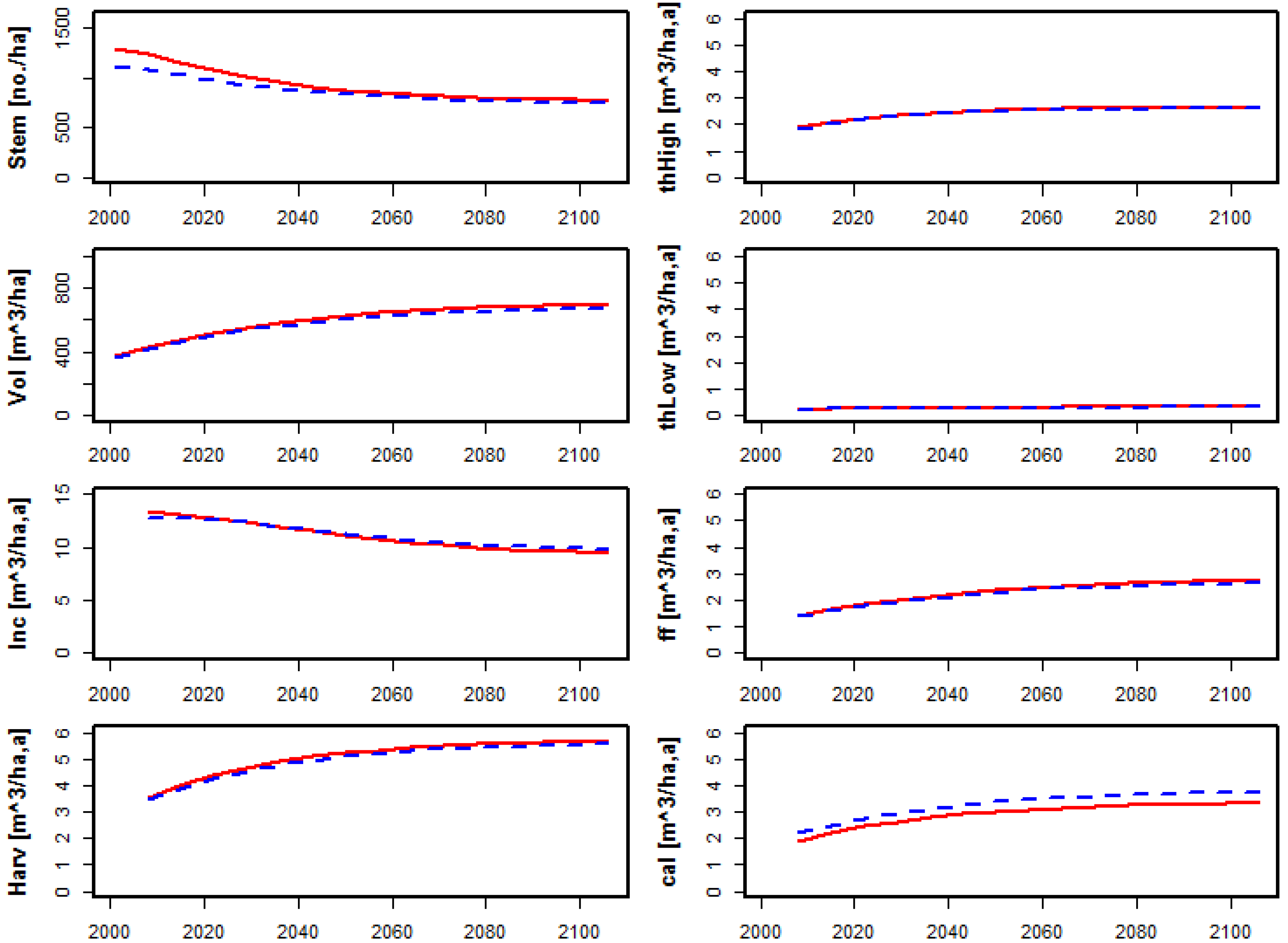
Simulations without management feature a reasonable development of standing volume, while the stem number development is harder to evaluate (Figure 1). Also, when introducing harvests, both the volume and the increment development are within a reasonable domain (Figure 2).

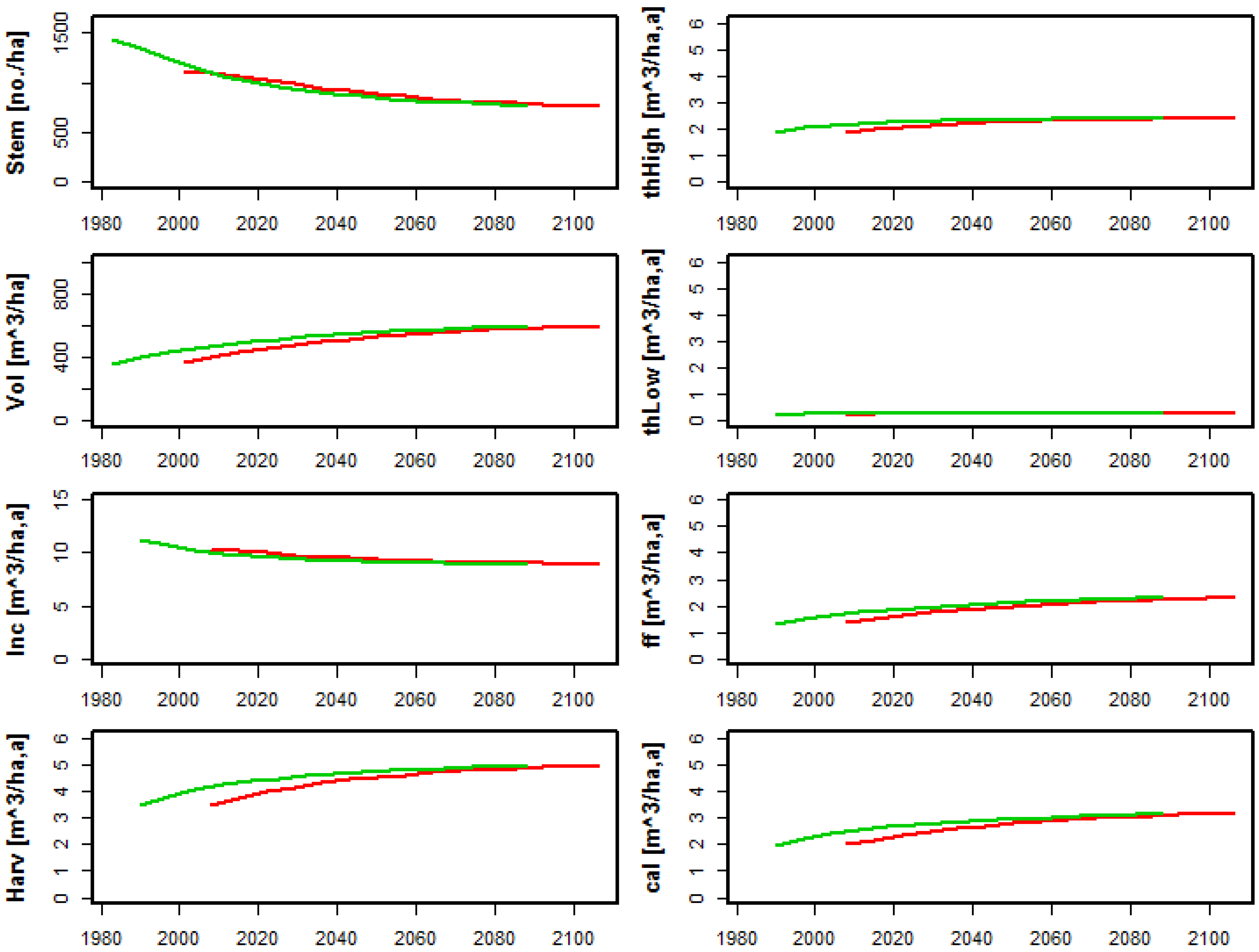
We are unsure how indicative the comparison between simulations based on the old and the new dataset. The differences could be due to differences in management and/or changes in inventory methods, as well as the high annual variation as mentioned before.

In the Austrian NFI the angle count method is used with a basal area factor of 4 (e.g., [30]). This means that discrete jumps in the stem number count and in volume occur when trees grow over a diameter threshold of the angle count method and thus grow into the sample. These jumps result in counter-intuitive transitions for the forests in the model. But one has to bear in mind that the input data for the model does not consist of forest stands, but of inventory plot data. This is a subtle but necessary distinction. So, technically, the output also consists of modeled inventory plot data. Since sampling has to employ thresholds as mentioned above, ingrowth causes jumps in the data which are not visible with the bare eye in the forest.

In the study, activity probabilities are estimated from the data. The primary target of the NFIs is to evaluate the growing stock. Often, NFI sampling design is too sparse to be used for reliable assessment of management activities, at least when applied over not that large areas. When the probabilities are estimated directly from an inventory on a “class by class” base, activity probabilities greater than zero will be estimated only for classes having at least one (but preferably several) plot in the data set. Classes with none or low number of observations can be biased. This problem could be solved by “filling in” the gaps in data with values derived from literature or expert evaluation. Another way, which has been employed in this study, is to calculate average values for the different activities and apply them over the entire state-space. This approach could and should be refined to yield more realistic management programs.

The model presented in this study shares a basic “stationarity” property with all models estimated from empirical data. If factors violating this property, like climate change, should be taken into account, additional information must be fed into the model, for example through transitions probabilities that can change over time. Technically this is doable, but the additional information is needed.

Intended for use, among others, on supranational level, it is essential that the model is not spatially extrapolated—it should be based on data from the entire region under study.

The approach presented here, to use an area-based transition model for large-scale analysis of UEA forests, is novel. The purpose of this paper is to demonstrate the concept. So far the concept is promising, but further work is needed before we could make a strong claim that the method works. In the next steps the model will be applied on data from several European countries inside the SC15 project currently running at the JRC.

5. Conclusions

In this paper a new concept for modeling uneven-aged forests (UEAF), i.e., forests which deviate from the even-aged structure has been presented. We have used the concept in an application to Austrian NFI data, which serves as a first test case. The results indicate that it could be worth further elaborating on the concept and the model. The modeled development of the forest is plausible and with the inclusion of several harvesting methods and calamities, there are sufficient possibilities for fine-tuning at hand.

The simple structure of the model is chosen so that the model can be applied to many diverse data sets. The model uses rather basic inventory data that should be available from any NFI. Thus many countries can use it with their NFI data and after some further development it would be possible to carry out large area estimates spanning several countries with different inventory systems.