Accuracy Assessment of Timber Volume Maps Using Forest Inventory Data and LiDAR Canopy Height Models

Abstract

Maps of standing timber volume provide valuable decision support for forest managers and have therefore been the subject of recent studies. For map production, field observations are commonly combined with area-wide remote sensing data in order to formulate prediction models, which are then applied over the entire inventory area. The accuracy of such maps has frequently been described by parameters such as the root mean square error of the prediction model. The aim of this study was to additionally address the accuracy of timber volume classes, which are used to better represent the map predictions. However, the use of constant class intervals neglects the possibility that the precision of the underlying prediction model may not be constant across the entire volume range, resulting in pronounced gradients between class accuracies. This study proposes an optimization technique that automatically identifies a classification scheme which accounts for the properties of the underlying model and the implied properties of the remote sensing support information. We demonstrate the approach in a mountainous study site in Eastern Switzerland covering a forest area of 2000 hectares using a multiple linear regression model approach. A LiDAR-based canopy height model (CHM) provided the auxiliary information; timber volume observations from the latest forest inventory were used for model calibration and map validation. The coefficient of determination (R² = 0.64) and the cross-validated root mean square error (RMSE_CV = 123.79 m³ ha⁻¹) were only slightly smaller than those of studies in less steep and heterogeneous landscapes. For a large set of pre-defined number of classes, the optimization model successfully identified those classification schemes that achieved the highest possible accuracies for each class.

1. Introduction

1.1. Context and Problem

Among the multitude of information that forest inventories are expected to provide [1], knowledge about available standing timber volume on the national, regional, as well as enterprise level is still of high interest. Since on these spatial levels, a full census is too cost-intensive and, in most cases, even practically unfeasible, a broad range of methods in the framework of sampling theory has been developed and applied to estimate this quantity [2,3,4]. The strength of forest inventory methods relying on design-based procedures is that (at least asymptotically) unbiased point and variance estimates can be obtained, and this without assuming the applied prediction models to be correct in the classical statistical (model-dependent) sense. An important advancement in increasing this accuracy without, at the same time, increasing the number of costly terrestrial samples has been achieved by combining terrestrial samples with auxiliary information provided by remote sensing data, so-called two-phase or double-sampling procedures [2,3,5,6]. In this context, especially airborne laser scanning (ALS) data have proven to provide a high degree of information for timber volume estimation [7,8,9]. It has recently been shown that the efficiency of two-phase sampling can be further increased by extending this procedure to stratification [10,11] or by using part of the auxiliary information exhaustively when remote sensing data are covering the entire inventory area [12]. The two-phase procedure is thus not restricted to large forest areas, but has also been applied in the context of small area estimation [13]. Given that the number of terrestrial samples in the small area is sufficiently large (i.e., one is not restricted to the application of synthetic estimations), even for small areas the accuracy specifications are ensured to be unbiased [14]. While these forest inventory methods have the advantage of supplying reliable accuracy specifications for their estimates, they do not provide information about the spatial distribution of the estimated quantity. However, the availability of spatially explicit stand information is of prime importance for efficiently locating forest management operations.

Accordingly, mapping the spatial distribution of standing timber volume has been the subject of various recent studies. The statistical models that have been used for mapping can be divided into parametric models, particularly linear regression models [15,16], and non-parametric models [17,18,19]. Among the non-parametric models, k‑NN imputation has become increasingly popular due to its simplicity and easy implementation [20]. k‑NN approaches have been investigated and applied in the model-dependent framework of forest inventory with promising results [21] and have also been used for the mapping of various forest attributes [22,23,24]. Haara and Kangas [25] compared the k‑NN method to linear regression in a simulation study and found the two methods to perform similarly well. Especially in the case where the relationship between observations and the auxiliary variable followed a linear trend, the regression model performed better than the k‑NN approach. Fehrmann, et al. [26] came to a similar result when comparing linear and linear mixed effect models to an instance-based k‑NN approach for single-tree biomass estimation. Also in their case, the performance of the k‑NN approach and the linear mixed model only differed marginally, and both methods were slightly superior to simple linear regression. On the other hand, they also confirmed that the application of k‑NN methods can be an effective and promising method if no a priori knowledge about the relationship between target and auxiliary variable(s) exists, particularly if the relationship is considered to be complex due to random and interaction effects. However, they also raised the question of whether a k‑NN approach should be used in situations where the functional relationship among variables is approximately known. Additionally, the performance of k‑NN estimation and its potential superiority to already existing methods has also been investigated in the design-based framework of forest inventory [27,28]. While in several cases, the proposed k‑NN estimator of the population mean achieved smaller errors than the Horwitz-Thompson estimator [3], the result also turned out to be dependent on the underlying model of the investigated population.

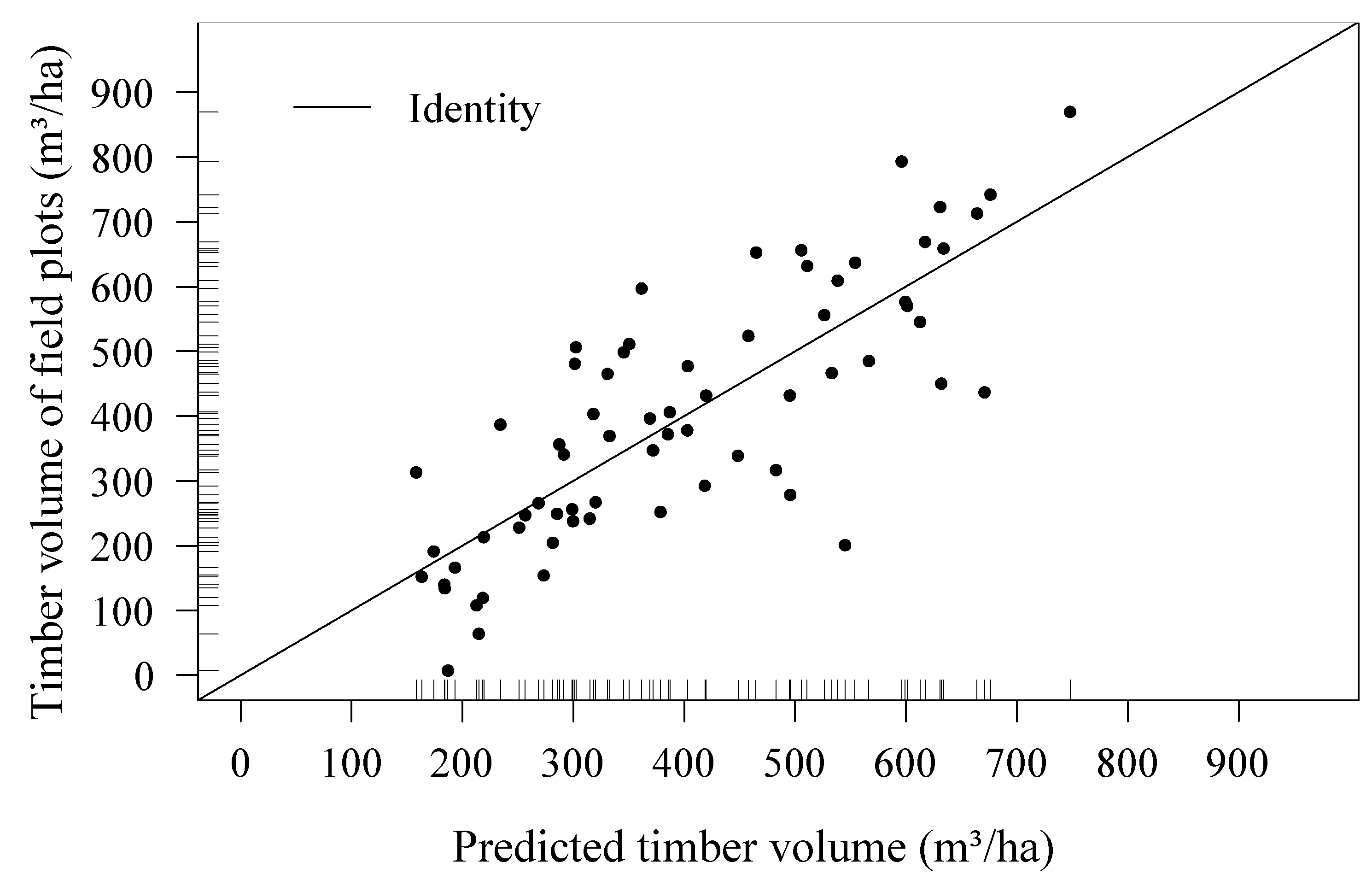
Irrespective of the model choice, a core issue of these mapping approaches is to characterize the accuracy of the resulting maps. If map predictions are made on a continuous prediction scale, the map precision is commonly characterized by quality parameters of the applied prediction model, such as the cross-validated root-mean-squared error (RMSE) and the coefficient of determination (R²). However, the derived map predictions are often visualized using constant class intervals in order to provide users, such as forest managers, with a better visual interpretation of the map. 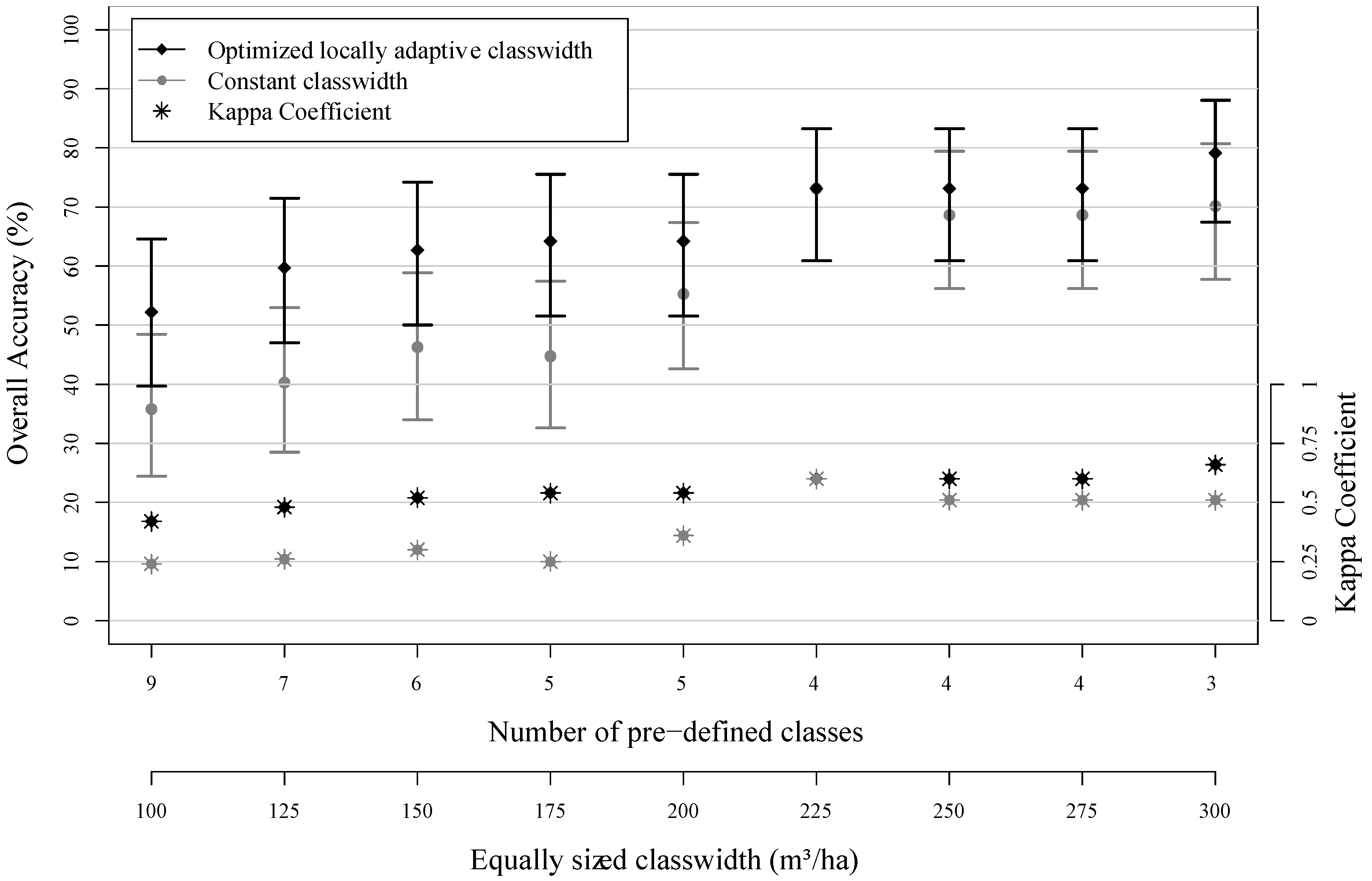In this case, it could be misleading to still use the previously mentioned RMSE and R² in order to provide information about the accuracy of resulting timber volume classes. This is because these parameters only describe the overall model performance on a continuous prediction scale, but do not quantify the accuracy of individual timber volume ranges (classes). A more appropriate validation strategy would then be to adopt the concept of confusion matrices, which provides a differentiated accuracy assessment (user’s and producer’s accuracy) for each particular volume class, as well as the complete mapping system. 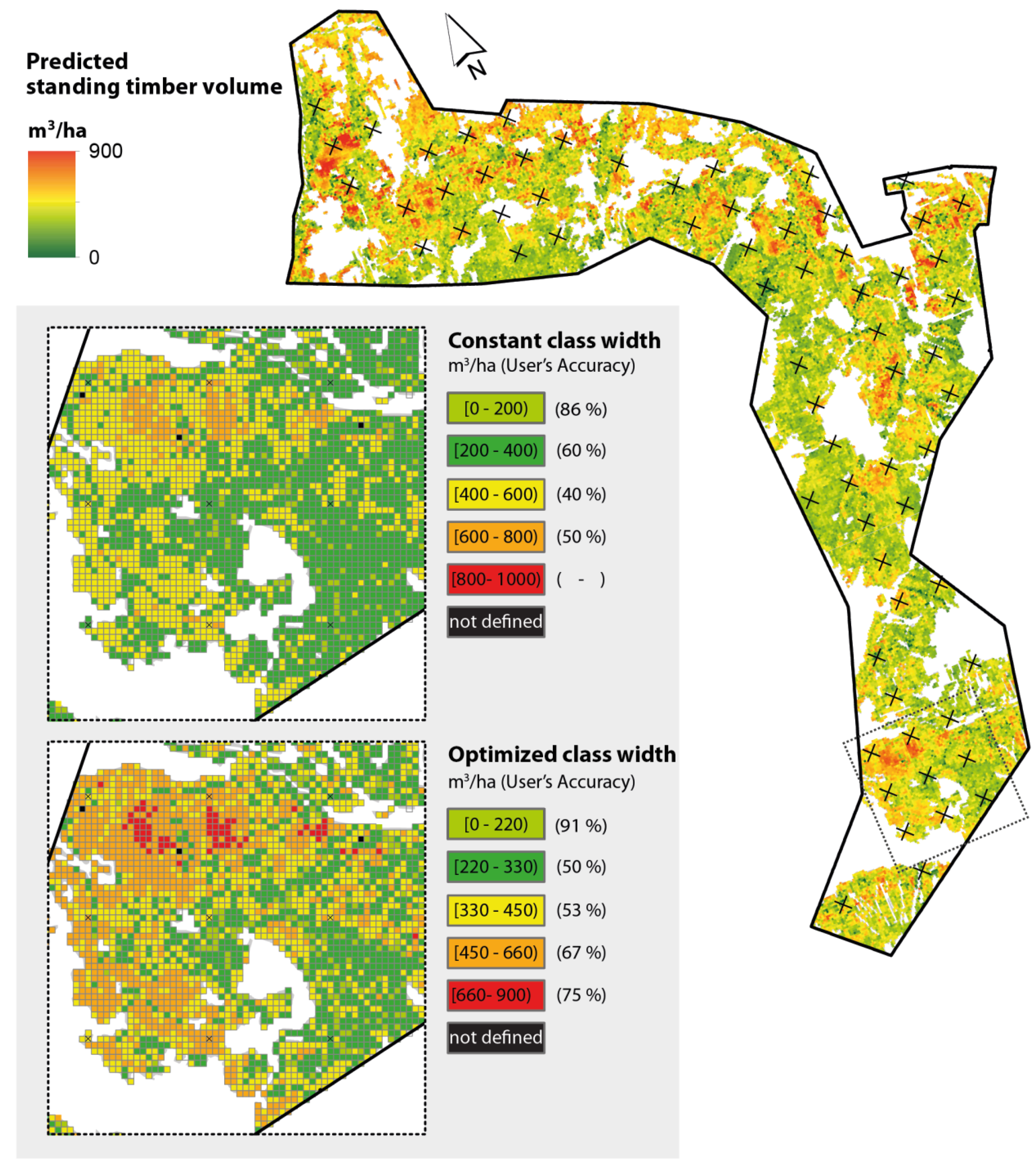Franco-Lopez, Ek and Bauer [17], for example, used these metrics. However, their classification scheme of constant class intervals exhibited a strong gradient of degrading class accuracies towards higher volume classes (most likely due to saturation effects in the remote sensing data). Such a severe gradient in class accuracies, however, reveals the following problems: (1) it implies that the chosen classification scheme with constant class intervals is not accounting for the fact that the performance of the underlying model may not be constant across the entire volume range; and (2) it severely hampers the usability of the maps in forest practice due to the high uncertainty within higher timber volume classes.

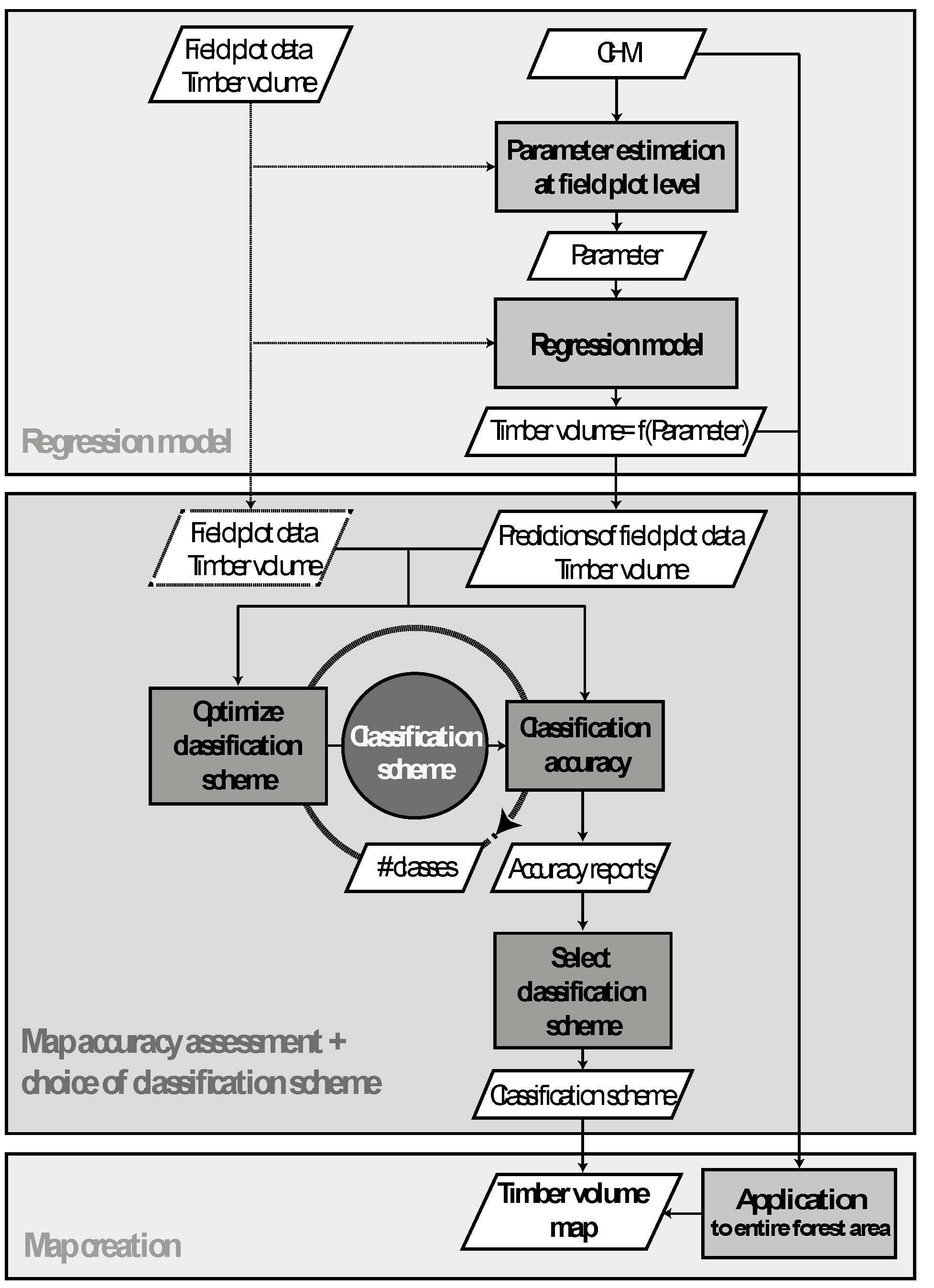
The motivation of this study was to improve the usability of volume maps for forest management operations by avoiding classification schemes of this kind. We hypothesized that this can be achieved by optimizing the class intervals with respect to the accuracy potential of the underlying prediction model. This implies using smaller class intervals in those volume ranges where the model ensures precise prediction performance and enlarging these intervals in ranges where the model performs worse. If the class boundaries are allocated according to this concept, it becomes possible to design classification schemes that provide highest possible accuracies for each class, while avoiding a severe gradient between class accuracies. This concept was investigated by implementing an optimization algorithm which can be applied to any type of prediction model that provides estimates on a continuous scale. Implicitly, the method also provides an additional option for evaluating the precision of prediction models.

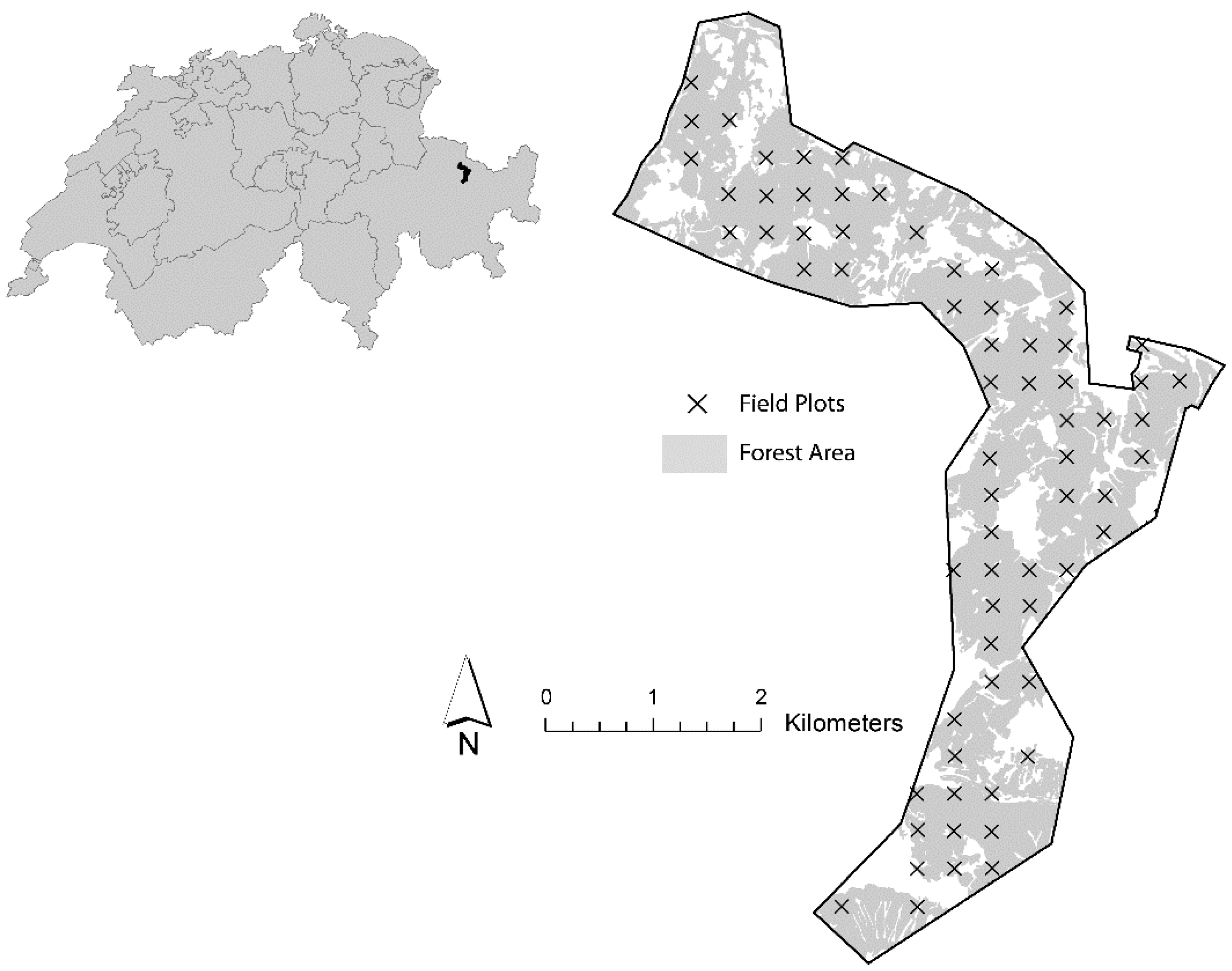
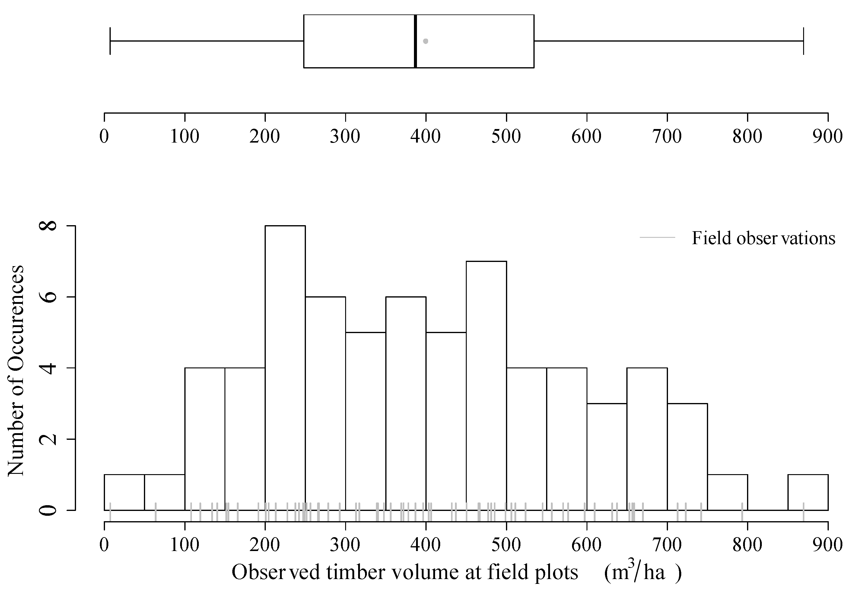
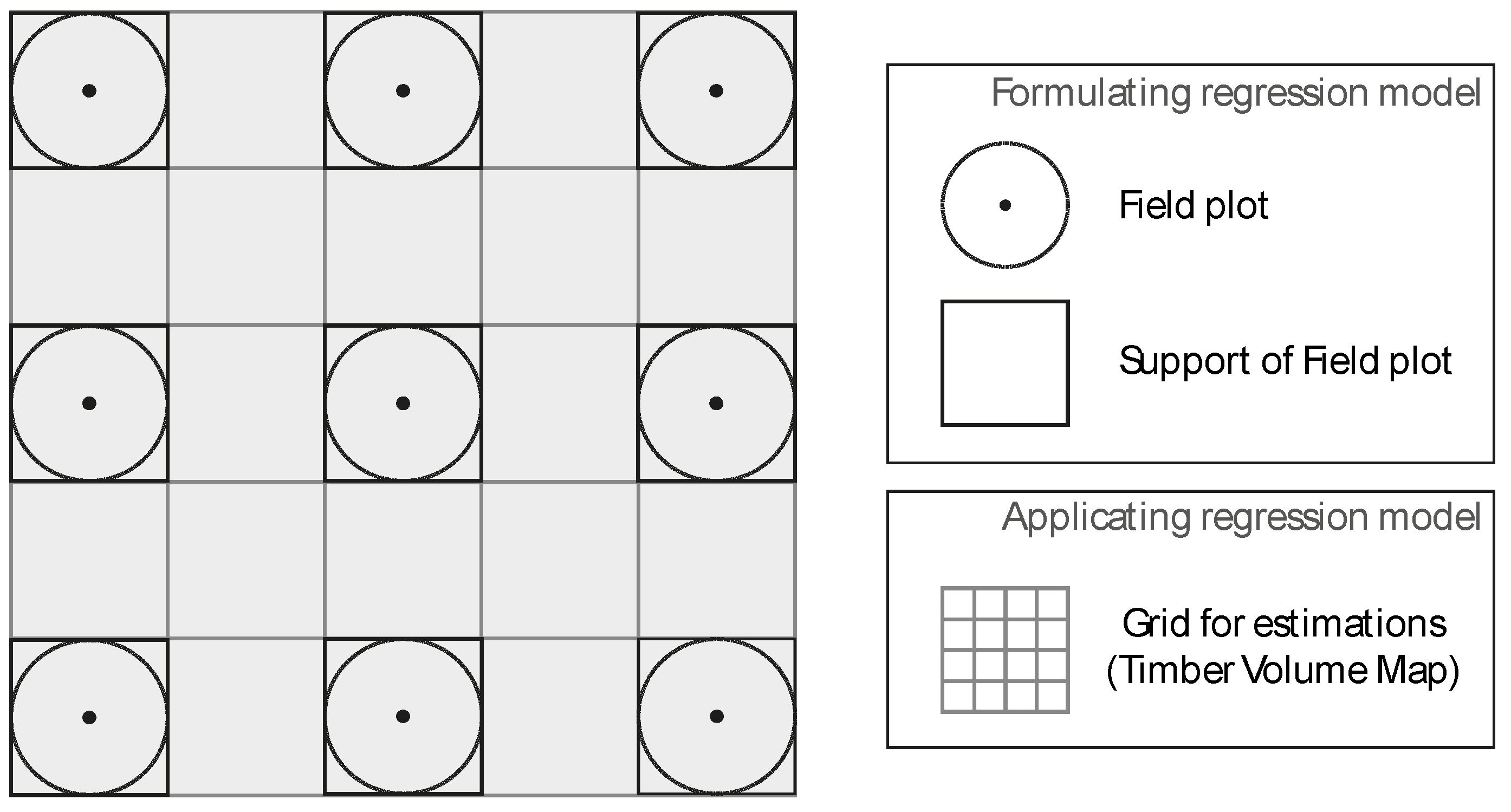
We demonstrate the method in a case study in the canton of Grisons using a LiDAR-derived canopy height model and regional forest inventory data. The workflow included: (1) the production of a map of estimated standing timber volume for the entire study area; (2) the calculation of reliable accuracy metrics for this map; and (3) the application of the proposed optimization algorithm in order to identify the classification schemes which provide the highest possible accuracies. In this particular case, we decided to use a multiple linear regression model, because most auxiliary variables exhibit a pronounced linear relationship to the terrestrial inventory [29]. Additionally, the number of available terrestrial observations in our study was small (n = 67) compared to similar studies, whereas it has been indicated that a good performance of k-NN requires larger datasets [26,30].

1.2. Background of Heuristic Search Methods

Heuristic Search Methods (HSMs) are often used when coping with combinatorial optimization problems [31] or, in general, problems whose structure cannot be satisfactorily represented and performed by means of classical optimization techniques, such as Linear Programming [32]. Basically, HSMs aim at improving an objective function by subsequent inspection and adoption of neighboring solutions. Inspection rules are often inspired by nature [31] and have the property of occasionally accepting inferior solutions for further inspection to avoid getting trapped within a local minimum or maximum. Simulated Annealing (SA) [33] is such an HSM, borrowing its accepting rule for inferior solutions from metallurgy. It is based on the assumption that a configuration of atoms in a metal can move to configurations of higher energy (i.e., inferior solution) with a certain probability at a given temperature. Given that probability is a function of temperature and energy difference to the inferior solution, SA adopts a cooling scheme that aims at “annealing” the metal to the point of minimum configuration energy (i.e., “objective function”). As opposed to classical optimization methods, optimality of HSM-derived solutions cannot be proven. However, one can assume to find a solution close to the true but unknown optimum if the heuristic is appropriately parameterized.

2. Materials and Methods

2.1. Materials

2.1.1. Study Area

The methods proposed in this article were applied to a study site located in the canton of Grisons, Eastern Switzerland (Figure 1). The site extends in the north-south direction between Klosters and Davos and covers a total area of 2887.39 hectares. According to a forest mask (in raster format) of the study site derived by the use of the Swiss TLM3D (Swiss Topographic Landscape Model) data with the approval of the Swiss Federal Institute of Topography (for details, see Hill [29]), the forest area of the study site comprises 1974.49 hectares (68.4%). The study site is located at an altitude between 900 and 2200 meters above sea level, and its relief is mainly characterized by rough terrain and steep slopes. Classifying the forest area of the study site according to the scheme given by Ott, et al. [34] revealed 49.7% of the forest area belonging to the high montane vegetation zone, 49.5% to the sub-alpine zone and 0.8% to the upper sub-alpine vegetation zone. Consequently, the forests within the study area were assumed primarily to consist of coniferous tree species, especially Norway spruce (Picea Abies).

Figure 1. Study site, including the distribution of the 67 field plots (regional forest inventory) that are part of the forest area derived from the TLM3D (Topographic Landscape Model) data (with approval of swisstopo JA100120/JD100042).

Figure 1. Study site, including the distribution of the 67 field plots (regional forest inventory) that are part of the forest area derived from the TLM3D (Topographic Landscape Model) data (with approval of swisstopo JA100120/JD100042).

2.1.2. Timber Volume Densities from Field Inventory

The methods applied in this study are based on timber volume densities obtained from terrestrial field surveys. For the study site, the timber volume densities were provided from field surveys of the latest regional forest inventory at the canton of Grisons and provided by the canton’s forest service. Any uncertainty of the timber volume densities associated with their acquisition was ignored (e.g., potential measurement errors). The forest area of the study site comprised 67 terrestrial plots, which had been surveyed in the year 2007 (Figure 1). Part of the survey was also the re-measurement of the plot centers with GPS technique. Unfortunately, no reliable information about the positional accuracy could be provided.

The field surveys were conducted using circular sample plots with their center (i.e., the sample point) belonging to a regional permanent systematic inventory grid with a mesh size of 500 m. This regional sampling scheme thus constitutes a sub-grid of the nation-wide terrestrial inventory grid of the National Swiss Forest Inventory (NFI) with a mesh size of 1.4 km. Each sample plot consists of two concentric circles with a plot area of 200 and 500 m² around the sample center. Within the inner circle (radius of 7.98 m), all trees with a diameter at breast height (DBH) larger than 12 cm were selected, whereas in the second circle (radius of 12.62 m), all trees with a DBH larger than 36 cm were included in the sample. Boundary and slope adjustments were performed on plot level. The explicit survey methods and the evaluation of the regional inventory surveys were identical to those of the NFI and can be found in detail in Brassel and Lischke [35] and Keller [36].

To obtain the standing timber volume on plot level, the overbark timber volume of each sample tree was estimated by measuring its DBH and using it as the main predictor variable in the tariff models provided by the NFI. These tariff models are based on the general function proposed by Hoffmann [37] and have been extended by further explanatory variables, such as the production region and additional tree and plot attributes [35]. The standing timber volume for each plot was then estimated according to the Horwitz-Thompson estimator, which provides an unbiased estimation of the actual timber volume on plot level [3]. The volume distribution of the 67 terrestrial observed field plots is illustrated in Figure 2, and a brief statistical summary is given in Table 1.

Figure 2. Terrestrial observed timber volume on plot level for all 67 sample plots of the study area (histogram bandwidth = 50 m³ ha⁻¹; origin = 0 m³ ha⁻¹).

Figure 2. Terrestrial observed timber volume on plot level for all 67 sample plots of the study area (histogram bandwidth = 50 m³ ha⁻¹; origin = 0 m³ ha⁻¹).

Table 1. Summary statistics of the timber volume observed at the 67 terrestrial sample plots (given in m³ ha⁻¹).

Range	Mean	Median	SD	n
7.3–869.57	399.4	386.9	194.94	67

Table 1. Summary statistics of the timber volume observed at the 67 terrestrial sample plots (given in m³ ha⁻¹).

Range	Mean	Median	SD	n
7.3–869.57	399.4	386.9	194.94	67

2.1.3. LiDAR Data

A LiDAR dataset covering the entire study area was acquired with a Riegl LMS Q 560 laser scanning system in the period September 11–15, 2010. The LiDAR acquisition was conducted as a part of a campaign to gather data for the Swiss National Park. A digital terrain model (DTM) and a digital surface model (DSM) with a spatial resolution of 0.5 m were computed by the provider Toposys by application of their company-internal processing software TopPit. Gaps in the DTM due to the absence of last echoes had not yet been interpolated. The average flight height was 700 m above ground, and the average echo density was 27 points m⁻². The provider specified the positional accuracy as <±0.50 m and the height accuracy as <±0.15 m. Further specifications of the LiDAR acquisition are summarized in Table 2.

Table 2. Specifications of the LiDAR data acquired in September, 2010, with a Riegl LMS Q 560 laser scanning system.

Beam deflection	Rotating mirror
Pulse Repetition Frequency (kHz)	70
Average Flying Altitude (m above ground)	700
Max. scan angle (°)	±15
Wavelength (nm)	1550
Beam divergence (mrad)	≤0.5
Average echo density (m−2)	27.4

Table 2. Specifications of the LiDAR data acquired in September, 2010, with a Riegl LMS Q 560 laser scanning system.

Beam deflection	Rotating mirror
Pulse Repetition Frequency (kHz)	70
Average Flying Altitude (m above ground)	700
Max. scan angle (°)	±15
Wavelength (nm)	1550
Beam divergence (mrad)	≤0.5
Average echo density (m−2)	27.4

2.2. Methods

The conceptual model in Figure 3 captures the general workflow of creating the timber volume map for the study area and the subsequent accuracy assessment. It consists of the following steps.

Figure 3. Conceptual model illustrating the workflow of producing the timber volume map and assessing its accuracy.

Figure 3. Conceptual model illustrating the workflow of producing the timber volume map and assessing its accuracy.

Step I: A regression model for predicting the standing timber volume in m³ ha⁻¹ is formulated using the terrestrial observed timber volume of the field plots as the response variable and parameters extracted from the canopy height model (CHM) at the respective plot locations as predictor variables. The model then allows for predicting the timber volume at each point of the CHM that lies within the inventory area.

Step II: The model predictions (Step I) at the plot locations are then compared to the corresponding field data. These comparisons are used to assess accuracy metrics of the timber volume map. Regarding the classification accuracies, which can be estimated under class representations of the timber volume map (i.e., timber volume classes), this part also comprises the application of an optimization model aiming to find an optimal classification scheme, i.e., the choice of class boundaries and class widths for a given number of classes.

Step III: The regression model (Step I) is applied to the entire study area, and the result is then represented using a classification scheme that best satisfies the required accuracies for map users (Step II).

2.2.1. Step I: Computation of Canopy Height Model

A canopy height model (CHM) with a spatial resolution of 0.5 m, completely covering the study site, was calculated by subtracting the LiDAR-acquired digital terrain model (DTM) from the digital surface model (DSM). As the DSM represents the elevation characteristics of the surface including vegetation and man-made structures, whereas the DTM describes only the elevation of the terrain, this operation equals removing the underlying terrain information from all features in the DSM. The height information of all objects in the CHM hence describes their estimated object height. Before calculating the CHM, an interpolation step for the DTM was crucial, since it exhibited a considerable amount of missing height information—most likely due to the absence of last pulse LiDAR returns over densely-covered forest areas. Missing height values in the DTM were predicted by applying an inverse distance weighting (IDW) interpolation algorithm [38]. Due to a locally varying number of adjacent missing raster values, the IDW algorithm was iteratively applied five times using varying neighborhood distances within which available height values were considered for interpolation. The use of small neighborhood distances aimed at providing a high amount of local precision where sufficient height values are available in the direct neighborhood of a missing value, whereas the use of large neighborhood distances was necessary for the interpolation of large gaps of missing values. Starting with a threshold distance of 2 neighbors, i.e., 1 m, and iteratively increasing the distance up to 20 neighbors, i.e., 10 m, all missing height values of the DTM were replaced by height predictions.

2.2.2. Step I: Regression Model

To predict the standing timber volume TV at location x, a multiple regression model was formulated using the observed timber volume of the field plots as the response variable and certain CHM metrics as predictor variables. The CHM metrics were extracted at all 67 field plots within squares of constant size, which were centered at the respective plot centers. To ensure high spatial consistency between the circular field plots and the CHM metrics, the square extent was chosen in order to tangentially circumscribe a field plot. The side length of a square was 25 m, resulting in an area of 625 m² compared to the field plot area of 500 m². In the following, these squares are also referred to as the support of the estimates. By analyzing the distribution of the raster values of the CHM within each square, we calculated the following metrics of the LiDAR CHM at each plot location: the mean, the standard deviation (SD), the maximum value, as well as the 25%, 75% and 90% quantiles (Q25, Q75, Q90). The reason for the choice of these parameters was that they have often been used as predictors for estimating timber volume of forest stands [7,8,39,40]. The calculations of these variables were also adjusted for boundary effects by only considering those raster values within a square that are covered by the forest mask (Section 2.1.1). Table 3 provides the main statistics for the observed CHM metrics at the 67 terrestrial sample plots. The regression model containing the maximum number of predictor variables conclusively reads as:

$$TV\left(x\right)={\beta }_0+{\beta }_{1}Mean\left(x\right)+{\beta }_{2}Sd\left(x\right)+{\beta }_{3}MAX\left(x\right)+{\beta }_{4}Q25\left(x\right)+{\beta }_{5}Q75\left(x\right) + {\beta }_{6}Q90\left(x\right)+\text{ ε}\left(\text{x}\right)$$

(1)

A variable selection procedure was applied in order to restrict the regression model to the most meaningful variables and to avoid an overfitting effect of the model [41] due to the small number of observations. As most of the predictor variables were considered to be correlated to each other (collinearity), criterion-based selection procedures, by means of AIC (Akaike information criterion) [42] and adjusted R‑square criteria [43], as well as Mallow’s C_p statistic [44], were preferred to the testing-based selection procedures relying on p-values.

Table 3. Summary statistics of the CHM metrics calculated at the 67 terrestrial sample plots (in meters).

Metrics	Range	Mean	Median	SD
Mean	2.26–26.03	12.07	11.31	5.89
SD	3.71–15.97	8.93	8.64	2.73
MAX	17.03–45.35	32.63	32.74	7.05
Q25	0–22.88	4.25	0.67	6.35
Q75	1.43–34.21	18.92	18.81	7.96
Q90	8.11–37.78	23.77	23.48	7.25

Table 3. Summary statistics of the CHM metrics calculated at the 67 terrestrial sample plots (in meters).

Metrics	Range	Mean	Median	SD
Mean	2.26–26.03	12.07	11.31	5.89
SD	3.71–15.97	8.93	8.64	2.73
MAX	17.03–45.35	32.63	32.74	7.05
Q25	0–22.88	4.25	0.67	6.35
Q75	1.43–34.21	18.92	18.81	7.96
Q90	8.11–37.78	23.77	23.48	7.25

2.2.3. Step II: Assessment of Map Accuracy

Prediction Performance

Assessing accuracy metrics of the timber volume map was realized by validating the timber volume predictions made by the regression model at the field plot locations using the corresponding observed timber volume of the field plots as reference data. Since the terrestrial sample was considered too small to be split into separate calibration and validation subsets, a leave-one-out cross-validation was performed to estimate the root-mean-squared error (RMSE) as a measure for the prediction performance of the timber volume map.

Classification Accuracy

We applied the concept of representing the timber volume map by prior defined timber volume classes (i.e., assigning the prediction of each raster cell to a prior defined interval). This representation has commonly been used by various research studies producing maps of forest parameters, such as basal area or timber volume [15,18,45], in order to facilitate the interpretability, as well as the readability of a map. We propose to treat this map representation as a classification procedure and, consequently, adopted the concept of confusion matrices to provide a differentiated assessment for each particular class as well as the complete mapping system. Using the available field data as reference data, we estimated the following accuracy metrics for the resulting classified timber volume map (for details, see Congalton and Green [46] and Richards [47]):

-

The overall accuracy (OAA) is the proportion of correctly classified pixels of the entire map. The true overall accuracy of the map is unknown, since we only have references for the classified raster cells at a small subspace of the map. The OAA is therefore estimated by the ratio of the total number of correctly classified pixels and the total number of reference/classified pixels. The 95% confidence interval for the OAA was calculated according to the binomial distribution.

-

The producer’s accuracy (PA) is a measure of the classification performance. It indicates the probability that if a ground observation belongs to a certain class, this class will be reflected in the map. The producer’s accuracy can be estimated for each class by dividing the number of correctly classified pixels of a class by the total number of reference pixels in this class.

-

The user’s accuracy (UA) of each class is the most interesting information for a user of the map. It indicates the probability that if the map shows a certain class, this class will actually be validated by a terrestrial survey. The producer’s accuracy is estimated by the number of correctly classified pixels in a class divided by the total number of classified data in this class.

-

Cohen’s kappa coefficient is a measure to assess to what degree the classification accuracy was realized by a chance agreement. The kappa coefficient ranges between −1 (accuracy was realized under pure chance agreement) and 1 (accuracy was reached by no chance agreement).

Class Selection Problem

One of the main benefits of classifying the timber volume map and assessing its classification accuracy is to provide information on the accuracies for individual timber volume ranges. However, classifying the model predictions into classes produces the problem of having to choose an appropriate classification scheme, i.e., choosing the class boundaries of the timber volume classes. A classic approach would be to use equally-sized classes with origin at zero and constant class width, but we consider three reasons not to do so: a constant class width (i) is likely to create classes for which no reference data are available, especially if the class width is chosen small; for such classes, PA and UA cannot be estimated, and the overall accuracy would give the user of the map an overoptimistic impression of the actual map precision; (ii) may separate a reference from its prediction (or vice versa) even if the two values were almost identical (i.e., their difference is very small and even negligible from a user’s point of view); (iii) does not account for saturation effects in the remote sensing data, occasionally leading to a strong gradient of degrading class accuracies towards higher volume classes. To overcome these problems, we propose a locally-adaptive selection of class boundaries which satisfies the following rules (Class Selection Problem):

Rule I: Choose the class boundaries to ensure that each timber volume class at least contains a minimum number of reference data. This also aims at using a smaller class width where a sufficient number of references is available (thus providing locally higher detail), whereas the class width is increased for regions where references are rare.

Rule II: Avoid cases where a reference and its (closely located) corresponding prediction are separated by a class boundary. This implies not only taking into account the distribution of the reference data, but also considering the distribution of their corresponding predictions. A slight adaptation of the class width may thereby increase the classification accuracy.

Optimization Model

The class selection problem (CSP) can be solved by repeatedly moving the boundaries and evaluating the resulting classification schemes until Rules I and II of the CSP are optimally satisfied. Since the number of combinations of alternative classification schemes can become big (e.g., 2.3 million alternatives to distribute four boundaries along a range of 10–900 m³ ha⁻¹ specified by a lower and an upper boundary and discretized into 88 steps of 10 m³ ha⁻¹), it risks becoming too computationally intensive to evaluate all alternatives. For this reason, we formulate the following multi-objective optimization model to automate the design of an (approximately) optimal classification scheme and solve it using Simulated Annealing (Section 1.2).

Its variables are specified as follows:

$$x_j\text{:class boundary value} j {\text{(m}}^3 {\text{ha}}^{-1}\text{)}$$

(2)

$$\text{class }j\text{ = (}{x}_j\text{,}{x}_{j+1}\text{) }, j=1,\mathrm{..},m+1$$

(3)

$$n_{ref,j}\text{:\# references/plots in class j}$$

(4)

$$y_{ij}=\{\begin{array}{l}1, V_{tp} \text{and} V_{pred}\text{at plot} i \text{in same class }j\hfill \\ 0, \text{otherwise}\hfill \end{array}$$

(5)

Where V_tp is the timber volume of terrestrial plot and Vpred the predicted timber volume. The decision variables x_j () define the class boundary positions. A class j is then defined via the interval which is bound to x_j and x_j+1 (3). The number of pre-defined classes is m. The number of reference data for class j is given by $n_{ref,j}$ and the binary indicator variable y_ij (5) captures whether V_tp and Vpred at plot i are assigned to the same class j (yes = 1, no = 0).

The optimization model can then be formulated as follows when n plots are subject to assignment:

$$MAX {\displaystyle \sum }_{j=1}^m{\displaystyle \sum }_{i=1}^n{y}_{ij}-w_1·{\displaystyle \sum }_{j=1}^m{\left(x_{j+1}-x_j\right)}^2- w_2·{\displaystyle \sum }_{j=1}^m{\left(\frac{n}{m}-n_{ref,j}\right)}^2$$

(6)

subject to:

$$x_{j+1}-x_j\ge t_w$$

(7)

$$x_j\ge 0, y_{ij}\in \left\{0;1\right\}$$

(8)

The objective function (Equation (6)) implements Rules I and II with three terms. The first term captures Rule II by maximizing for the number of cases where terrestrial observed volumes V_tp and corresponding estimated volumes V_pred are assigned to the same class j. In principle, the first term can be maximized by proposing a “super class” covering almost the entire range. The second term is thus introduced to penalize the selection of a “super class” by minimizing for local class widths, thereby also accounting for Rule I. This is realized by minimizing the square class width for each class j. Equation (7) limits the minimum class width to a threshold t_w (m³ ha⁻¹) and concurrently satisfies that x_j+1 is chosen bigger than x_j. The third term captures Rule I and aims at equally distributing the reference data over all classes by minimizing the squared difference between the average number of plots per class and the actual number of reference data for each class j.

Both the second and the third terms are implemented as penalty terms for the first term that aims at maximizing the number of correctly classified plots. The corresponding weights w₁ and w₂ can be used to control the emphasis of both penalty terms and provides the user with the possibility to prefer one of the three objectives within the optimization process.

In order to find an appropriate choice for the weight factors, several weights have to be evaluated to achieve satisfactory classification schemes. In our study, we decided to give the weights equal emphasis (w₁ = w₂ = 2). Class boundary selection was restricted to a range discretized into 10 m³ ha⁻¹ units to reduce the problem size and simultaneously create useable class boundaries in the final classification scheme. A satisfying alternative was then identified by picking out the best overall solution from 100 runs of Simulated Annealing, where each run included the computation of 1000 alternatives.

2.2.4. Step III: Computation of the Timber Volume Map

After model selection, the regression model (Section 2.2.2) was applied at any location x of the CHM, i.e., over the entire study area. We chose the design of the timber volume map in accordance with the setup of the regression model: the spatial resolution of the map was defined as the size of the support used for ground calibration, i.e., 25 × 25 m. We further orientated the map in such a way that the supports at the field plots actually became an almost exact subset of all raster cells of the timber volume map. Within each of the raster cells, the CHM metrics used in the regression model were calculated by the same procedure as described in Section 2.2.2 (i.e., by the same support and technique) and then used to predict the timber volume. The estimated value was then assigned to the entire raster cell, resulting in a timber volume map with a spatial resolution of 25 × 25 m. The entire procedure is again illustrated in Figure 4.

The design of the map as proposed here has two main advantages that allow for relying on the provided classification accuracy metrics: (i) each estimate of a raster cell is based on exactly the same support that was used to calibrate the prediction model; and (ii) as the reference data are an (almost) exact subset of the map raster cells, this allows for a valid accuracy assessment of the classified timber volume map [46].

Another advantage of the map design is that it is in perfect agreement with the inventory design of the generalized two-phase regression estimator proposed by Mandallaz et al. [12], where part of the auxiliary information is derived exhaustively over the entire inventory area. It thereby provides a link between the derived timber volume map and sample designs of classical forest inventory.

Once the timber volume map was calculated for the entire study area, each raster cell of the map, still carrying estimates on a continuous scale, was classified into timber volume classes according to a classification scheme (Step II, Section 2.2.3).

Figure 4. Schematic design of the timber volume map.

Figure 4. Schematic design of the timber volume map.

3. Results

3.1. Regression Model

Performing individual simple linear regressions revealed that all predictor variables derived from the CHM were correlated to the field-obtained timber volume on plot level. Here, the highest coefficient of determination (R²) was achieved by the variable mean (R² = 0.5). A forward, backward, as well as bidirectional selection procedure according to minimize the AIC all revealed mean, standard deviation, maximum value and the 75% quantile as the model of choice (adjusted R² = 0.62, AIC = 646.4). These predictor variables also revealed a significant influence on the field-obtained timber volume (individual parameter t-test, 5% significance level). The model was also suggested by Mallow’s C_p and the adjusted R²-criterion selection procedure. Summary statistics of the model are presented in Table 4. The estimated timber volume $\widehat{TV}\left(x\right)$ at location x was consequently calculated according to the following regression model formula:

$$\widehat{TV}\left(x\right)= 228.83+ 62.76·Mean\left(x\right) + 76.65·Sd\left(x\right) - 19.59·Max\left(x\right) - 33.44·Q75\left(x\right)$$

(9)

Figure 5 shows the predicted timber volume on plot level plotted against the observed timber volume of the field plots. The leave-one-out cross-validated RMSE_CV of the regression model was 123.79 m³ ha⁻¹ and, thus, only slightly larger than the RMSE without cross-validation (115.5 m³ ha⁻¹).

Figure 5. Model-predicted timber volume on plot level against the observed timber volume of the 67 field plots; the distribution of the predictions and observations are also indicated on the respective axis.

Figure 5. Model-predicted timber volume on plot level against the observed timber volume of the 67 field plots; the distribution of the predictions and observations are also indicated on the respective axis.

Table 4. Summary statistics of the regression model.

Predictors	AIC	R2	Adjusted R2	Mallow’s Cp	RMSECV	Model Range
Mean *, SD *, Max *, Q75 *	646.4	0.64	0.62	2.56	123.79	0–900m3 ha−1

* Indicating a significant influence of a predictor variable based on individual parameter t-test (5% significance level).

Table 4. Summary statistics of the regression model.

Predictors	AIC	R2	Adjusted R2	Mallow’s Cp	RMSECV	Model Range
Mean *, SD *, Max *, Q75 *	646.4	0.64	0.62	2.56	123.79	0–900m3 ha−1

* Indicating a significant influence of a predictor variable based on individual parameter t-test (5% significance level).

3.2. Assessment of Map Classification Accuracy

The classification accuracies described in Section 2.2.3 were estimated for nine possible constant class widths (100, 125, 150, 175, 200, 250, 275 and 300 m³ ha⁻¹), which were assumed to be of interest for representing the timber volume map. We applied the optimization model (Section 2.2.3) for each of those constant class widths in order to find a better classification scheme using the same number of corresponding classes, but locally adaptive class widths. The accuracies were then also estimated for the best-found classification schemes.

Figure 6 provides a graphical summary of the results, giving the overall accuracies with their 95% confidence intervals, as well as the kappa coefficients.

In all cases but one, the optimized locally-adapted class widths led to a higher overall classification accuracy compared to the corresponding constant class width. However, the 95% confidence intervals revealed that the overall accuracies using the constant class widths were, in all cases, not significantly different from their corresponding optimized alternatives (i.e., the confidence intervals are overlapping). In other words, even if the differences between the two accuracies seemed in several cases to be quite distinct, the true (but unknown) overall accuracies of the corresponding maps could actually be identical. However, with respect to the overlapping areas of the confidence intervals, the probability of acquiring a better overall accuracy by using the locally-adapted class widths was highest for smaller constant class widths (i.e., for larger numbers of classes). Interestingly, at the same time, a constant class width of 225 m³ ha⁻¹ (four classes) was also the best-found solution for locally-adapted class widths. In all cases but one, the kappa coefficients were higher under the application of the optimized class widths, even more distinct for larger numbers of classes (i.e., smaller constant class widths).

Figure 6. Overall accuracies with 95% confidence intervals and corresponding kappa coefficients for a pre-defined number of classes, calculated for constant and locally-adapted class widths.

Figure 6. Overall accuracies with 95% confidence intervals and corresponding kappa coefficients for a pre-defined number of classes, calculated for constant and locally-adapted class widths.

We further compared the properties of the confusion matrices obtained by the use of constant and corresponding locally-adapted class widths, especially with respect to the estimated producer’s and user’s accuracies. The producer’s, as well as the user’s accuracies under the optimized classification schemes were consistently higher than those of the corresponding constant class width approach. A phenomenon that, in several cases, occurred for the constant class width approach was that some of the classes did not include at least one prediction. This phenomenon especially concerned the classes comprising the upper scale region of the field data where the number of reference data was small. Consequently, the producer’s accuracy for these classes was zero, whereas the user’s accuracy is not even defined for this case (Section 2.2.3). The reason for this undesired property of the confusion matrix is likely to be that the fit of the regression model for the upper timber volume range was rather poor due to a limited number of field data or/and a saturation effect in the CHM (i.e., beyond a certain canopy height, different timber volumes cannot longer be discriminated by the regression model). The constant class width approach did, however, not account for this effect, whereas the optimization model proposed larger class widths for the upper-range classes, including a larger number of field data and predictions. An illustration of the findings described can be found in Table 5 and Table 6, using a constant class width of 200 m³ ha⁻¹ (five locally-adapted classes, respectively). The described locally-adaptive classification scheme provided a satisfactory trade-off between the number of classes and classification accuracies and was therefore exemplary used for the visualization of the timber volume map (Figure 7).

Table 5. Constant class width of 200 m³ ha⁻¹ (five timber volume classes); OAA (±95% confidence interval) (%): 55.22 (42.58, 67.4); kappa: 0.36; square sum of class widths: 200,000.

Classes	Class Width	Producer’s Accuracy	User’s Accuracy	No. of References
(0, 200)	200	60	85.71	10
(200, 400)	200	72	60	25
(400, 600)	200	40	40	20
(600, 800)	200	45.45	50	11
(800, 1000)	200	0	-	1

Table 5. Constant class width of 200 m³ ha⁻¹ (five timber volume classes); OAA (±95% confidence interval) (%): 55.22 (42.58, 67.4); kappa: 0.36; square sum of class widths: 200,000.

Classes	Class Width	Producer’s Accuracy	User’s Accuracy	No. of References
(0, 200)	200	60	85.71	10
(200, 400)	200	72	60	25
(400, 600)	200	40	40	20
(600, 800)	200	45.45	50	11
(800, 1000)	200	0	-	1

Table 6. Optimized locally-adapted class width for five timber volume classes; OAA (±95% confidence interval) (%): 64.18 (51.53, 75.53); kappa: 0.54; square sum of class widths: 176,600. Class widths smaller than 200 m³ ha⁻¹ are indicated by *.

Classes	Class Width	Producer’s Accuracy	User’s Accuracy	No. of References
(0, 220)	220	76.92	90.91	13
(220, 330)	110 *	61.54	50	13
(330, 450)	120 *	57.14	53.33	14
(450, 660)	210	66.67	66.67	21
(660, 900)	240	50	75	6

Table 6. Optimized locally-adapted class width for five timber volume classes; OAA (±95% confidence interval) (%): 64.18 (51.53, 75.53); kappa: 0.54; square sum of class widths: 176,600. Class widths smaller than 200 m³ ha⁻¹ are indicated by *.

Classes	Class Width	Producer’s Accuracy	User’s Accuracy	No. of References
(0, 220)	220	76.92	90.91	13
(220, 330)	110 *	61.54	50	13
(330, 450)	120 *	57.14	53.33	14
(450, 660)	210	66.67	66.67	21
(660, 900)	240	50	75	6

Additionally, we investigated how often the locally-adaptive class widths were capable of satisfying Rules I and II of the optimization model (Section 2.2.3) more successfully than their constant class width counterparts. This was done by comparing the respective sum of squared class widths (second term of Equation 6), as well as the respective squared difference between the average number of plots per class and the actual number of reference data for each class (third term of Equation 6). It turned out that, particularly for the larger constant class widths (175, 200, 225, 250, 275 and 300 m³ ha⁻¹), the locally-adapted approach worked very successfully for both objectives: in six out of nine cases, each objective was better solved by the locally-adaptive approach, and in five out of nine cases, the optimization approach even succeeded in both objectives simultaneously.

Figure 7. Volume map with model-predictions on a continuous scale for the entire study area covering 2000 hectares of forest with a spatial resolution of 25 meters; the subareas show the classified volume map using a constant class width of 200 m³ ha⁻¹ (upper) and locally-optimized class widths for five classes (lower).

Figure 7. Volume map with model-predictions on a continuous scale for the entire study area covering 2000 hectares of forest with a spatial resolution of 25 meters; the subareas show the classified volume map using a constant class width of 200 m³ ha⁻¹ (upper) and locally-optimized class widths for five classes (lower).

3.3. Calculation of the Timber Volume Map

Figure 7 shows the timber volume map for the entire study area estimated by the application of the regression model (Equation (9)). An undesired property of the map was the occasional appearance of negative predictions, which are most likely caused by the negative signs of two of the regression coefficients (Equation (9)). Additionally, the upper range of the predictions of the entire map (1002 m³ ha⁻¹) turned out to exceed the upper valid model range (900 m³ ha⁻¹). The values of these raster cells were consequently changed into “Not Available” (NA). The map was additionally classified according to a constant class width of 200 m³ ha⁻¹, as well as to the corresponding optimized classification scheme presented in Section 3.2. As the classification schemes were also based on the valid model range, cells whose predictions did not cover any of the pre-defined classes were consequently marked as “not defined” in the classified map. The number of these cases was, however, small compared to the total number of predicted cell values of the entire volume map (170 of 31,622 raster cells, i.e., 0.5%).

4. Discussion

4.1. Assessment of Map Accuracy

A core issue of this study was to use a class representation of continuous map predictions to estimate accuracy metrics of individual timber volume ranges (user’s and producers accuracies). An evaluation for a large number of classification schemes revealed that the class accuracies can vary according to (i) which class width is used, (ii) how the class boundaries are chosen and (iii) a combination of both aspects. This variation in accuracy is not indicated by metrics such as the cross-validated RMSE of the prediction model, which can, however, be used to describe the overall prediction performance. When investigating the map for explicit timber volume ranges, purely relying on RMSE or R² metrics could, however, lead to over- or underestimation of the provided accuracy. Building the map according to classes and, consequently, estimating their individual accuracies is therefore considered a valuable step towards coping with the uncertainty of such maps.

4.2. Class Selection by Optimization Model

Regarding the choice of appropriate classes to represent the timber volume map, the proposed optimization model turned out to be of high value. While the overall accuracies between the optimized class width and constant class width approach did not differ significantly on a 5% significance level, the true benefit of the optimized class width approach were the properties of the confusion matrices thus obtained. The proposed classes revealed a more uniform distribution of references among the classes, ensuring that the estimated producer’s and user’s accuracies of each class were estimated by the highest possible number of references. The class width was thus successfully chosen smaller where a sufficient number of reference data were available, leading to a higher degree of detail and, with respect to an optimized adaptation of the class boundaries, without a loss of accuracy in those classes. In many of the evaluated classification schemes, the adaptation of the class boundaries led to higher producer’s and user’s accuracies compared to those obtained under constant class widths.

The optimization model has yet provided a method which allows for (i) finding an optimal classification scheme for a given number of classes and (ii) finding a number of classes, such that the class accuracies are acceptable for a user. If forest managers are interested in identifying stands with timber volumes greater than a selected minimum, perhaps for possible thinning treatments, one of the class boundaries can be fixed to that minimum volume.

While the maximization for the number of predictions and references included in the same class (Rule II, Section 2.2.3) gives a more realistic representation of the underlying regression model, one could argue that optimizing for this objective can lead to an “overfitting” of the confusion matrix and, thus, to an increased generalization error of the accuracy metrics. This could not be investigated, since an appropriate method of bootstrapping and cross-validating for this kind of classification process has yet to be implemented. However, one could also slightly change the optimization model in order to optimize only for Rule I (i.e., to locally achieve smaller class widths and an even distribution of the reference data over the classes).

4.3. Regression Model

In the present study, the mean of the canopy height turned out to be the best predictor, providing an R² of already 0.5. The fit was further improved to an adjusted R² of 0.62 by extending the model using the predictor variables standard deviation, maximum height and the 75% quantile. This, however, came at the price of losing interpretability of the model (negative signs of some regression coefficients), as well as the occurrence of negative predictions in the timber volume map. The latter reassuringly happened only for 141 of 31,622 pixels (0.4%). To avoid negative predictions, we also computed the regression model using the log-response of the terrestrial timber volume and then calculated the map by back-transformation of the log-predictions into the original scale [48]. The log-response model, however, tended to predict unrealistically large timber volume values (up to 2400 m³ ha⁻¹), exceeding the valid model range in 267 cases (0.16%) and, thus, not providing an improvement in prediction performance. The use of a log-response or non-linear regression model is also methodically sound in the design-based framework, with the restriction that only the variance under the external model assumption [3] can be calculated. This is because the design-based variance using the g-weight technique [12,14] is only available within linear models on the original scale. Within the model-dependent framework, other alternatives to ensure non-negative predictions can be the use of nonlinear logistic regression models [49] or k‑NN approaches. One could also consider the alternative use of external models (e.g., taken from literature) based on data that provide, for example, a larger model range or better coverage of a required timber volume range. It would be statistically sound to estimate the classification accuracies by applying an external model and consequently validating its classified predictions by available reference data of the study site. Using such models in the design-based framework of inventory would, however, again require calculating the variance under the external model approach.

4.4. Availability and Quality of Reference Data

In the present study, we used existing forest inventory data as reference and validation data, instead of acquiring these data in a special campaign. While this is in general both time and cost saving, the number of available reference data for calibrating the regression model and for validating the timber volume map was considerably limited, finally resulting in large confidence intervals of the accuracy metrics. However, in order to produce maps for operational forest management, probably over considerably large areas, one will realistically always depend on the use of existing inventory data due to limited financial resources. It should also be mentioned that the proposed methods assume the nominal coordinates of all field plots to be equal to the actual, true location of acquisition. This is in practice almost never the case, due to potential location errors, which can still be in the range of up to 10 meters, even under the use of GPS technique [50,51]. Although the remote sensing data can reveal positioning errorsas well, they can be expected to be considerably smaller than the largest possible GPS location errors occasionally caused by dense vegetation and shielding of GPS reception on the ground. However, severe location errors should have appeared as outliers (or even leverage points) in the regression model. Since, in our case, neither the cross-validation nor an inspection of the regression model revealed any such outliers, the severity of location errors was assumed to be small. However, the R² of the regression model is expected to be higher if the exact positions of the plot centers are known [52], and the same can be assumed for the classification accuracies under the restriction that the locally-adaptive class width must be recomputed if the model is changed.

5. Conclusions

The methods proposed in this study provide better knowledge about the actual accuracy of a timber volume map. The classification of predictions into classes and the consequent computation of classification accuracy metrics improved the knowledge about the map accuracy, especially the accuracies of timber volume intervals. Additionally, considering the distribution of the reference data, as well as their corresponding predictions turned out to be key factors in choosing an appropriate classification scheme: the application of optimized locally-adaptive class widths ensured good statistical properties of the confusion matrices and also led to higher class accuracies and kappa coefficients compared to the approach of using constant class widths. The proposed methods, including the optimization of classification schemes, are thus not restricted to maps based on linear regression models, but can be applied to a larger class of prediction methods (e.g., k-NN estimation). Finally, the proposed design of the timber volume map was considered to be crucial for the reliability of the estimated accuracy metrics. Another advancement of the entire map set up is that the continuous map predictions can be directly used in the framework of design-based inventory methods. For example, several raster cells of the volume map could be merged, e.g., to 0.5 or one hectare, and the resulting larger cell could be used for true small area (synthetic) estimation [14]. We expect this approach to also solve the problem of negative predictions. The design-based confidence intervals thus obtained for these estimates could then serve as a measure for local accuracy. The accuracy assessment of timber volume classes could also improve an automatic delineation of possible harvesting units by additionally considering the probability of each raster cell belonging to a certain class.

References

1. McRoberts, R.E.; Tomppo, E.O.; Næsset, E. Advances and emerging issues in national forest inventories. Scand. J. For. Res. 2010, 25, 368–381. [Google Scholar]
2. Gregoire, T.G.; Valentine, H.T. Sampling Strategies for Natural Resources and the Environment; Chapman & Hall/CRC: Boca Raton, FL, USA, 2008. [Google Scholar]
3. Mandallaz, D. Sampling Techniques for Forest Inventorie; Chapman & Hall/CRC: Boca Raton, FL, USA, 2008; p. 247. [Google Scholar]
4. Schreuder, H.T.; Wood, G.B.; Gregoire, T.G. Sampling Methods for Multiresource Forest Inventory; John Wiley & Sons: New York, NY, USA, 1993. [Google Scholar]
5. Cochran, W.G. Sampling Techniques, 2 ed.; John Wiley & Sons: New York, NY, USA, 1977. [Google Scholar]
6. Köhl, M.; Magnussen, S.; Marchetti, M. Sampling Methods, Remote Sensing and Gis Multiresource Forest Inventory; Springer: Berlin/Heidelberg, Germany, 2006. [Google Scholar]
7. Holmgren, J. Prediction of tree height, basal area and stem volume in forest stands using airborne laser scanning. Scand. J. For. Res. 2004, 19, 543–553. [Google Scholar] [CrossRef]
8. Næsset, E. Predicting forest stand characteristics with airborne scanning laser using a practical two-stage procedure and field data. Remote Sens. Environ. 2002, 80, 88–99. [Google Scholar] [CrossRef]
9. Næsset, E. Airborne laser scanning as a method in operational forest inventory: Status of accuracy assessments accomplished in scandinavia. Scand. J. For. Res. 2007, 22, 433–442. [Google Scholar] [CrossRef]
10. Saborowski, J.; Marx, A.; Nagel, J.; Böckmann, T. Double sampling for stratification in periodic inventories—Infinite population approach. For. Ecol. Manag. 2010, 260, 1886–1895. [Google Scholar] [CrossRef]
11. Von Lüpke, N. Approaches for the Optimisation of Double Sampling for Stratification in Repeated Forest Inventories. Ph.D. Thesis, Georg-August-Universität Göttingen, Göttingen, Germany, 2013. [Google Scholar]
12. Mandallaz, D.; Breschan, J.; Hill, A. New regression estimators in forest inventories with two-phase sampling and partially exhaustive information: A design-based monte carlo approach with applications to small-area estimation. Can. J. For. Res. 2013, 43, 1023–1031. [Google Scholar] [CrossRef]
13. Breidenbach, J.; Astrup, R. Small area estimation of forest attributes in the norwegian national forest inventory. Eur. J. For. Res. 2012, 131, 1255–1267. [Google Scholar] [CrossRef]
14. Mandallaz, D. Design-based properties of some small-area estimators in forest inventory with two-phase sampling. Can. J. For. Res. 2013, 43, 441–449. [Google Scholar] [CrossRef]
15. Tonolli, S.; Dalponte, M.; Vescovo, L.; Rodeghiero, M.; Bruzzone, L.; Gianelle, D. Mapping and modeling forest tree volume using forest inventory and airborne laser scanning. Eur. J. For. Res. 2011, 130, 569–577. [Google Scholar] [CrossRef]
16. Van Aardt, J.A.; Wynne, R.H.; Scrivani, J.A. Lidar-based mapping of forest volume and biomass by taxonomic group using structurally homogenous segments. Photogramm. Eng. Remote Sens. 2008, 74, 1033–1044. [Google Scholar]
17. Franco-Lopez, H.; Ek, A.R.; Bauer, M.E. Estimation and mapping of forest stand density, volume, and cover type using the k-nearest neighbors method. Remote Sens. Environ. 2001, 77, 251–274. [Google Scholar] [CrossRef]
18. Latifi, H.; Nothdurft, A.; Koch, B. Non-parametric prediction and mapping of standing timber volume and biomass in a temperate forest: Application of multiple optical/lidar-derived predictors. Forestry 2010, 83, 395–407. [Google Scholar]
19. Nothdurft, A.; Saborowski, J.; Breidenbach, J. Spatial prediction of forest stand variables. Eur. J. For. Res. 2009, 128, 241–251. [Google Scholar] [CrossRef]
20. Magnussen, S.; Tomppo, E. The k-nearest neighbor technique with local linear regression. Scand. J. For. Res. 2014, 29, 120–131. [Google Scholar] [CrossRef]
21. McRoberts, R.E.; Tomppo, E.O.; Finley, A.O.; Heikkinen, J. Estimating areal means and variances of forest attributes using the k-nearest neighbors technique and satellite imagery. Remote Sens. Environ. 2007, 111, 466–480. [Google Scholar] [CrossRef]
22. Beaudoin, A.; Bernier, P.Y.; Guindon, L.; Villemaire, P.; Guo, X.J.; Stinson, G.; Bergeron, T.; Magnussen, S.; Hall, R.J. Mapping attributes of canada’s forests at moderate resolution through knn and modis imagery. Can. J. Forest. Res. 2014, 44, 521–532. [Google Scholar] [CrossRef]
23. Chirici, G.; Corona, P.; Marchetti, M.; Mastronardi, A.; Maselli, F.; Bottai, L.; Travaglini, D. K-NN forest: A software for the non-parametric prediction and mapping of environmental variables by the k-nearest neighbors algorithm. Eur. J. Remote Sens. 2012, 45. [Google Scholar] [CrossRef]
24. Tomppo, E. The finnish multi-source national forest inventory-small area estimationand map production. In Forest Inventory; Springer: Berlin, Germany, 2006; pp. 195–224. [Google Scholar]
25. Haara, A.; Kangas, A. Comparing k Nearest Neighbours Methods and Linear Regression—Is There Reason to Select One over the Other? Math. Comput. For. Nat. Res. Sci. 2012, 16, 50–65. [Google Scholar]
26. Fehrmann, L.; Lehtonen, A.; Kleinn, C.; Tomppo, E. Comparison of linear and mixed-effect regression models and a k-nearest neighbour approach for estimation of single-tree biomass. Can. J. For. Res. 2008, 38, 1–9. [Google Scholar] [CrossRef]
27. Baffetta, F.; Corona, P.; Fattorini, L. Design-based diagnostics for k-nn estimators of forest resourcesthis article is one of a selection of papers from extending forest inventory and monitoring over space and time. Can. J. For. Res. 2010, 41, 59–72. [Google Scholar] [CrossRef] [Green Version]
28. Baffetta, F.; Fattorini, L.; Franceschi, S.; Corona, P. Design-based approach to k-nearest neighbours technique for coupling field and remotely sensed data in forest surveys. Remote Sens. Environ. 2009, 113, 463–475. [Google Scholar] [CrossRef] [Green Version]
29. Hill, A. Comparison of Small Area Estimators in Forest Inventory Using Airborne Laserscanning Data Vergleich von Kleingebietsschätzern in der Waldinventur Unter Benutzung Von Flugzeugerhobenen Laserscanner Daten. Master Thesis, Georg-August-University, Göttingen, Germany, 2013. [Google Scholar]
30. Magnussen, S.; Tomppo, E.; McRoberts, R.E. A model-assisted k-nearest neighbour approach to remove extrapolation bias. Scand. J. For. Res. 2010, 25, 174–184. [Google Scholar] [CrossRef]
31. Pirlot, M. General local search methods. Eur. J. Oper. Res. 1996, 92, 493–511. [Google Scholar] [CrossRef]
32. Rayward-Smith, V.J. Modern Heuristic Search Methods; Wiley: Chichester, UK, 1996; p. 294. [Google Scholar]
33. Kirkpatrick, S.; Gelatt, C.D.; Vecchi, M.P. Optimization by simulated annealing. Science 1983, 220, 671–680. [Google Scholar] [CrossRef] [PubMed]
34. Ott, E.; Frehner, M.; Frey, H.U.; Lüscher, P. Gebirgsnadelwälder.Ein Praxisorientierter Leitfaden für eine Standortgerechte Waldbehandlung; Paul Haupt: Bern, Switzerland; Stuttgart, Germany; Wien, Austria, 1997. [Google Scholar]
35. Brassel, P.; Lischke, H. Swiss National Forest Inventory: Methods and Models of the Second Assessment; Swiss Federal Institute of Forest, Snow and Landscape Research WSL: Birmensdorf, Zurich, Switzerland, 2001. [Google Scholar]
36. Keller, M.R. Swiss National Forest Inventory. Manual of the Field Survey 2004–2007; Swiss Federal Institute of Forest, Snow and Landscape Research WSL: Birmensdorf, Zurich, Switzerland, 2011; p. 269. [Google Scholar]
37. Hoffmann, C. Die berechnung von tarifen für die waldinventur. Forstwiss. Cent. 1982, 101, 24–36. [Google Scholar] [CrossRef]
38. Isaaks, E.; Srivastava, R. Applied Geostatistics; Oxford University: London, UK, 2011. [Google Scholar]
39. Lefsky, M.A.; Cohen, W.B.; Acker, S.A.; Parker, G.G.; Spies, T.A.; Harding, D. Lidar remote sensing of the canopy structure and biophysical properties of douglas-fir western hemlock forests. Remote Sens. Environ. 1999, 70, 339–361. [Google Scholar] [CrossRef]
40. Magnussen, S.; Eggermont, P.; LaRiccia, V.N. Recovering tree heights from airborne laser scanner data. For. Sci. 1999, 45, 407–422. [Google Scholar]
41. Draper, N.R.; Smith, H. Applied Regression Analysis; Wiley: New York, NY, USA, 1966. [Google Scholar]
42. Akaike, H. Information Theory and An Extension of the Maximum Likelihood Principle. In Proceedings of the Second International Symposium on Information Theory, Akademinai Kiado, Budapest, Hungary; 1973; pp. 267–281. [Google Scholar]
43. Srivastava, A.K.; Srivastava, V.K.; Ullah, A. The coefficient of determination and its adjusted version in linear regression models. Econom. Rev. 1995, 14, 229–240. [Google Scholar] [CrossRef]
44. Mallows, C.L. Some comments on Cp. Technometrics 1973, 15, 661–675. [Google Scholar]
45. Clementel, F.; Colle, G.; Farruggia, C.; Floris, A.; Scrinzi, G.; Torresan, C. Estimating forest timber volume by means of “low-cost” lidar data. Ital. J. Remote Sens. Riv. Ital. Di Telerilevamento 2012, 44, 125–140. [Google Scholar] [CrossRef]
46. Congalton, R.G.; Green, K. Assessing the Accuracy of Remotely Sensed Data: Principles and Practices; Lewis Publications: Boca Raton, FL, USA, 1999; p. 137. [Google Scholar]
47. Richards, J.A. Remote Sensing Digital Image Analysis: An Introduction, 5th ed.; Springer: Berlin, Germany, 2013. [Google Scholar]
48. Beauchamp, J.J.; Olson, J.S. Corrections for bias in regression estimates after logarithmic transformation. Ecology 1973, 54, 1403–1407. [Google Scholar] [CrossRef]
49. McRoberts, R.E.; Næsset, E.; Gobakken, T. Inference for lidar-assisted estimation of forest growing stock volume. Remote Sens. Environ. 2013, 128, 268–275. [Google Scholar] [CrossRef]
50. Mauro, F.; Valbuena, R.; Manzanera, J.A.; García-Abril, A. Influence of global navigation satellite system errors in positioning inventory plots for tree-height distribution studies. Can. J. For. Res. 2010, 41, 11–23. [Google Scholar] [CrossRef]
51. Steinmann, K.; Mandallaz, D.; Ginzler, C.; Lanz, A. Small area estimations of proportion of forest and timber volume combining lidar data and stereo aerial images with terrestrial data. Scand. J. For. Res. 2012, 28, 373–385. [Google Scholar] [CrossRef]
52. Fuller, W.A. Measurement Error Models; Wiley: New York, NY, USA, 1987. [Google Scholar]