Article

Improving the Simulation Accuracy of the Net Ecosystem Productivity of Subtropical Forests in China: Sensitivity Analysis and Parameter Calibration Based on the BIOME-BGC Model

1
State Key Laboratory of Subtropical Silviculture, Zhejiang A & F University, Hangzhou 311300, China
2
Key Laboratory of Carbon Cycling in Forest Ecosystems and Carbon Sequestration of Zhejiang Province, Zhejiang A & F University, Hangzhou 311300, China
3
School of Environmental and Resources Science, Zhejiang A & F University, Hangzhou 311300, China
*
Author to whom correspondence should be addressed.
Forests 2024, 15(3), 552; https://doi.org/10.3390/f15030552
Submission received: 27 January 2024 / Revised: 10 March 2024 / Accepted: 11 March 2024 / Published: 18 March 2024
(This article belongs to the Section Forest Inventory, Modeling and Remote Sensing)

Abstract

:
Subtropical forests have strong carbon sequestration potential; however, the spatiotemporal patterns of their carbon sink are unclear. The BIOME-BGC model is a powerful tool for forest carbon sink estimation while the numerous parameters, as well as the localization, limit their application. This study takes three typical subtropical forests (evergreen broadleaf forest, EBF; evergreen needleleaf forest, ENF; and bamboo forest, BF) in China as examples, assesses the sensitivity of 43 ecophysiological parameters in the BIOME-BGC model both by the Morris method and the extended Fourier amplitude sensitivity test (EFAST), and then evaluates the net ecosystem productivity (NEP) estimation accuracy based on the dataset of the fiveFi long-term carbon flux sites of those three typical forests from 2000 to 2015. The results showed that (1) both sensitivity analysis methods can effectively screen out important parameters affecting NEP simulation while the Morris method is more computationally efficient and the EFAST is better in the quantitative evaluation of sensitivity. (2) The highly sensitive parameters obtained using the two methods are basically the same; however, their importance varies across sites and vegetation types, e.g., the most sensitive parameters are k for the EBF and ENF and Ract25 for the BF, respectively. (3) The optimized parameters successfully improved the NEP simulation accuracy in subtropical forests, with average correlation coefficients increased by 25.19% and normalized root mean square error reduced by 21.74% compared with those simulated by original parameters. This study provides a theoretical basis for the optimization of process model parameters and important technical support for accurate NEP simulations of subtropical forest ecosystems.

1. Introduction

Forests are the largest carbon reservoirs in terrestrial ecosystems and help maintain global carbon balance and mitigate global climate change [1,2]. Net ecosystem productivity (NEP), an indicator of carbon sinks in terrestrial ecosystems, is the difference between the net primary productivity (NPP) of vegetation and heterotrophic respiration [3] and can quantitatively describe the net carbon exchange between terrestrial ecosystems and the atmosphere.
Models coupled with remote sensing capabilities merge the inherent advantages of remote sensing, such as real-time, dynamic, broad spatially synchronous monitoring, and multiresolution attributes with the quantitative simulation capabilities of models that address diverse aspects of the ecosystem’s carbon cycle. This fusion facilitates expansive simulations of the carbon cycle processes, establishing it as a paramount methodology for extensive forest carbon sink monitoring [4]. The process model is developed based on vegetation physiological ecology and ecosystem processes and functions [5]. As a paradigmatic ecosystem process model, BIOME-BGC simulates physiological and ecological processes, such as photosynthesis, respiration, and decomposition, across a range of scales [6]. Its intrinsic mechanistic rigor, high degree of integration, and excellent extrapolation capabilities [7] render it an invaluable asset for terrestrial ecosystem studies, with broad applications both within and beyond national borders [8,9,10]. However, many of the model’s input parameters cannot be derived from real measurements and errors in parameter estimation lead to large uncertainties in the simulation results. Therefore, the targeted optimization and calibration of key parameters can significantly reduce the workload of model calibration and improve model accuracy and predictive capability [11].
Global sensitivity analysis can simultaneously test the influence of multiple parameter changes and interactions between parameters on the model output and is necessary for model optimization and parameter calibration. Qualitative global sensitivity analyses provide a qualitative measure of the effect of model parameters on simulation outcomes and include the Fourier amplitude sensitivity test (FAST) [12] and the Morris method [13]. Quantitative global sensitivity analysis calculates the contribution rate of model parameters to the uncertainty of simulation outcomes and mainly includes the Sobol method [14] and the extended Fourier amplitude sensitivity test (EFAST) [15]. The Morris method can screen out sensitive parameters under a small sample size and has good applicability to models with many analysis parameters and large computational loads. It is a qualitative global sensitivity analysis method widely used at present. Wang et al. [16] employed the Morris method to identify the most critical parameters in a C-RIVE model under various nutrient conditions. DeJongea et al. [17] demonstrated that the computationally less costly Morris method can effectively screen for sensitive parameters of the CERES-maize crop model under different irrigation conditions. The EFAST combines the capabilities of the Sobol method, which calculates the parameter interactions, and the efficient sampling of the FAST. The EFAST analyzes not only the impact of each parameter’s variation on model output but also the influence of interactions between multiple parameters on model outcomes [18], finding widespread application in numerous nonlinear models. Li et al. [19] used the EFAST to assess the contributions of various input parameters in the DSSAT-CERES model to wheat yield and quality. Gilardelli et al. [20] employed the EFAST to evaluate the impact on the yield of parameter value variations in crop models simulating different crops under climate change. The assessment of sensitive parameters affecting the model using suitable methods is a prerequisite for model calibration and optimization, as well as the basis for localized application of the model.
The NEP of subtropical forest ecosystems in the East Asian monsoon region, which plays an important role in the global carbon cycle and carbon sink function, is 0.72 Pg C·a−1 [21]. China is an important distribution area for subtropical forests and evergreen broad-leaved forests and evergreen coniferous forests are widely distributed in subtropical China [21]. The bamboo forest is known as the second-largest forest in the world and its carbon stock accounts for ~0.94% of the global forest ecosystem carbon stock [22]. China is known as the “world’s bamboo kingdom”, with abundant bamboo resources widely distributed in subtropical areas, such as Zhejiang, Fujian, and Jiangxi.
Simulations of the carbon and water cycles of various ecosystems found great uncertainty while monitoring subtropical forest carbon sinks, mainly for the following reasons. (1) When the BIOME-BGC model has been used to simulate the carbon cycle, the bamboo forest has not been treated as a separate forest, introducing uncertainty into the simulation. (2) Many studies have reported sensitivity analyses of BIOME-BGC parameters. Yan et al. [23] applied the EFAST to analyze and obtain sensitive parameters affecting the gross primary productivity (GPP) of the Changbaishan Forest. Tatarinov et al. [24] analyzed the effects of site and physiological–ecological parameters on the NPP of temperate forests in Europe. However, previous studies have predominantly focused on discerning the effects of parameter modifications on outputs, such as GPP and NPP. Notably, there is a paucity of evidence of the implications of model parameter fluctuations for NEP outputs, which amplifies the uncertainties in the simulation outcomes. (3) The calibration parameters of the BIOME-BGC model vary for different vegetation types under different environmental and site conditions. Raj et al. [25] investigated the sensitivity of the parameters in the BIOME-BGC model to the carbon fluxes of Douglas fir in the Speulderbos forest in the Netherlands and found that FLNR and FRC:LC (New fine root C: leaf C) were the key factors. Liu et al. [26] found that k was the most sensitive to estimate carbon fluxes in rubber forest ecosystems on Hainan Island. And FLRN was a low-sensitivity parameter but FRC:LC was not found to be the key control parameter. Kkumar and Raghubanshi [27] showed that FLNR and FRC:LC contributed less to the modeling of carbon fluxes in dry tropical forests. However, these studies suggest that the results of sensitivity analyses in other regions cannot be directly applied to simulate the carbon cycle in subtropical forests because of the climate, soil, and vegetation types.
In this study, we investigated the sensitivity of the physiological ecological parameters in the BIOME-BGC model to simulate the NEP of three forest ecosystems at five sites in subtropical China using the Morris method and EFAST. We aimed to screen key control parameters, improve the accuracy of model calibration, and provide scientific support for accurately assessing the carbon sink capacity of subtropical forests.

2. Materials and Methods

2.1. Study Area

Subtropical China (22–34° N, 98–122° E) is located south of the Qinling and Huaihe rivers, north of the Leizhou Peninsula, and east of the Hengduan Mountains, accounting for approximately 1/4 of the country’s national land area (Figure 1). Subtropical China belongs to the humid monsoon zone on the east coast, with the average annual temperature ranging from −1 to 24 °C and the average annual precipitation ranging from 450 to 2125 mm. The terrain is low in the west and high in the east and the soil type is reddish-yellow loam. Typical subtropical forests are evergreen broadleaf forests (EBFs), evergreen needleleaf forests (ENFs), and bamboo forests (BFs). Therefore, five flux observation sites were selected in this study for these three forests to participate in the parameter sensitivity analysis and parameter optimization, including Dinghushan (DHS), Tianmushan (TMS), Qianyezhou (QYZ), Anji (AJ), and Taihuyuan (THY). The information in Table 1.

2.2. Subtropical Forest Flux Data and Meteorological Factors

Because the flux observation station may have problems, such as data loss caused by equipment failure, in order to ensure the accuracy and continuity of the observation data, we selected the data from 2000 to 2015, which are more complete than other years. Therefore, daily-scale NEP and meteorological data were collected from five observation stations from 2000 to 2015 and the meteorological factors were daily maximum temperature (°C), daily minimum temperature (°C), daily precipitation (mm), daily relative humidity (%), and total solar radiation (WJ-m−2). Data from the DHS, TMS, and QYZ sites were obtained from ChinaFlux (http://chinaflux.org, accessed on 10 September 2023). Data from the AJ and THY sites were obtained from the Carbon Flux Observing System, including the open-circuit vorticity correlation system and the conventional meteorological observation system. A detailed account of the instrumentation and the associated apparatus was provided by Mao et al. [28]. The observations from the carbon flux tower were sampled at a frequency of 10 Hz and processed into daily-scale NEP as follows. The flux data were corrected using the method described by Papale et al. [29] and processed using EdiRe software. Data interpolation of missing data was performed using the nightly data-based approach [30,31], whereby if the proportion of missing data to the total daily data volume was >20%, then the data for that day were discarded; if it was <20%, then the daily average value of NEP was multiplied by 24 to obtain the daily value of NEP. Daily meteorological data are half-hourly statistically recorded by the conventional meteorological observation system into daily-scale data.

2.3. Soil and Topographic Data

The soil data included the percentage of soil silt content and available soil water-holding capacity, which were calculated based on the soil texture obtained from the Harmonized World Soil Database (HWSD1.2) for the subtropics. Subtropical soil texture data were obtained from the Chinese soil dataset with a spatial resolution of 0.05° provided by the HWSD1.2. The topographic data included the Chinese subtropical digital elevation model and slope and direction data. Digital elevation model data were obtained from The ASTER Global Digital Elevation Model version 3 [32] and the slope and slope direction were calculated using ArcMap10.2. Finally, corresponding soil and terrain data were extracted based on the latitude and longitude of the flux observation sites.

2.4. BIOME-BGC Model Description

BIOME-BGC is a physiological–ecological process model that evolved from the forest-BGC model [33] (Figure 2). The model applies mechanistic modeling of photosynthetic enzymatic reactions [34], using a two-leaf model for the canopy and simulating GPP through the Farquhar Photosynthesis and Leuning Conductance models. Autotrophic respiration is divided into two components: maintenance and growth. Maintenance respiration was calculated using a model that relates plant tissue nitrogen content to the Q10 relationship. Growth respiration was obtained by multiplying the photosynthetic fixed organic matter of each plant tissue by a fixed coefficient. NEP is the difference between NPP and heterotrophic respiration; NPP is obtained by subtracting autotrophic respiration from GPP. Heterotrophic respiration originates mainly from the decomposition of soil organic matter and plant litter. The input data driving this model consist of three parts: (1) initialization files, such as elevation data, soil data, and atmospheric CO2 concentration; (2) meteorological data at a daily scale, including minimum and maximum temperatures, precipitation, solar radiation, and saturated water vapor pressure; and (3) physiological and ecological parameters.
The BIOME-BGC model adopts a constant rate of growth and dieback for evergreen forests, does not consider the effects of bamboo forest size or anthropogenic disturbances on carbon cycling, and is not suitable for simulating carbon cycling in bamboo forest ecosystems [35]. Mao et al. [36] improved the BIOME-BGC model by introducing a forest age factor, bamboo whip carbon pool, bamboo forest climatic processes, the carbon allocation factor, and four bamboo forest management measures (fertilizer application, bamboo shoot digging, bamboo tip hooking, and bamboo harvesting).
The model was run in two steps, firstly a spin-up simulation, starting with very low initial values of carbon and nitrogen and running until the ecosystem reached a steady state, judged by an annual change in the soil carbon pool of ≤0.0005 kg·m−2 [37]. The spin-up results were used as the initial values for carbon, nitrogen, and water reservoirs in the normal simulation. In this study, the original BIOME-BGC model was used for the EBF and ENF carbon cycle simulations and the improved BIOME-BGC model was used for the BF carbon cycle simulation.
Figure 2. Structure of the BIOME-BGC model [38].
Forests 15 00552 g002

2.5. Sensitivity Analysis

Sensitivity analyses of the physiological and ecological parameters of BIOME-BGC were conducted using the Morris method and EFAST to qualitatively and quantitatively analyze the effects of the input parameters on NEP.

2.5.1. Morris Method

The Morris method calculates the sensitivity of each parameter by differentiation, assuming that the system model is Y =  f(x1, x2,…, xk) and k is the number of dimensions of the model parameters. Morris’s method first maps the range of values of each parameter to the interval [0, 1] and divides it into p levels, which constitute the sample space of the k dimensions and p levels. The elemental effects of each parameter are defined as follows:
S i = [ y ( x 1 , , x i 1 , x i + Δ , x i + 1 , , x k ) y ( x ) ] Δ
where Δ is a value between 1 / p 1 and 1 1 / ( p 1 ) .
Using this method to calculate the elemental effects for each variable one by one requires a total of k + 1 operations on the model; however, a single calculation does not show the whole of the sample space so it is usually necessary to generate different samples to calculate the Si several times and to find the mean µi and the standard deviation σi the formula is as follows:
μ i = j = 1 r S i j r
σ i = j = 1 r ( S i j μ i ) 2 r
where r is the number of repetitions.
To eliminate the positive and negative due to non-monotonic functional relationships of µi values canceling each other out, μ i    is usually used for evaluation [39]; see Equation (4):
μ i * = j = 1 r | S i j | r
where μ i reflects the sensitivity of xi and the larger the μ i , the greater its influence on the model output results; σi reflects the interaction between xi and other parameters.

2.5.2. EFAST

The EFAST quantifies the contribution of parameters to the variance of the model results. The model was assumed to be Y = f ( x ) = f (xi,j,k,…) and the input parameter was (xi,j,k,…) By estimating the sensitivity of the variance contribution of each input parameter change to the output Y , the total variance of the model output VY can be decomposed as follows [40]:
V Y = i V i + i j V i j + + i j k V i j k
where VY is the total variance of the model results Y ; Vi is the variance of xi; and V i j ~ V i j k is the variance of the parameter interactions.
V i = V [ E ( Y / x i ) ]
where E ( Y / x i ) is the conditional expectation of Y over x i and V [ E ( Y / x i ) ] is the variance of the conditional expectation of Y over xi.
V i j = V [ E ( Y / x i , x j ) ] V i V j
where E ( Y / x i , x j ) is the conditional expectation of Y over x i and x j and V [ E ( Y / x i , x j ) ] is the variance of Y over x i and x j .
The variance of the conditional expectation is called the main effect, which reflects the significance of x i to the variance of the model results Y . Therefore, the sensitivity index can be obtained by calculating the ratio of the variance of each parameter and parameter interaction to the total variance. The first-order sensitivity index Si can reflect the direct contribution of x i to the total variance of the model results and can be defined as:
S i = V i V Y
Similarly, the second-order sensitivity index Sij for x i is defined as:
S i j = V i j V Y
The total sensitivity index SiT is the sum of the sensitivity indices of each order, reflecting the direct contribution of x i and the indirect contribution to the total variance of the model output through the interaction coupling between the parameters:
S i T = S i + S i j + + S i j k
The greater the sensitivity index of x i ; the greater the contribution of the parameter to the model results Y , both directly and indirectly through the interaction coupling between parameters; and the greater the explanatory power for the variance of changes in the model results.

2.5.3. Parameter Value Establishment

This study focused on the physiological and ecological parameters of this model. First, the parameters involved in the sensitivity analysis were selected and their baseline values were determined. The fire mortality rate was set to zero and the parameters were used to characterize markers, such as vegetation type or photosynthetic characteristics; parameters with fixed combination ratios were not included. Finally, 38, 38, and 43 parameters were selected for the EBF, ENF, and BF to participate in the sensitivity analysis, which were categorized in this study (Table 2 and Table 3). The baseline values of the parameters were obtained using three methods: (1) some of the parameters were obtained by actual measurements in the sample plots, (2) other plant physiological parameters were obtained by conducting literature searches for each parameter and calculating the mean values, and (3) the parameter values of the EBF and ENF provided by White et al. [41] were used for parameters that could not be determined from the literature. Secondly, the value range of each parameter was determined because BIOME-BGC did not give the specific value range of each parameter so we floated 20% on the basis of the benchmark value of each parameter [41], setting the value range of the parameters as (x − Δx, x + Δx), where x is the benchmark value of the parameter Δx = 0.2x using a uniform distribution; the parameters are independent of each other, as shown in Supplementary Materials (Tables S1 and S2) [41,42,43,44,45,46,47,48,49,50,51,52].

2.5.4. Sensitivity Analysis Steps

The sensitivity analysis was conducted with SimLab (Version 2.2) (Figure 3). The value range, distribution form, and sampling time were set for each parameter. Using the Monte Carlo method to generate parameter samples by random sampling of the parameters in Table 2, the distribution form of each parameter was assumed to be uniform [53]. The sampling number of the Morris method was r × ( K + 1 ) ( K is the number of parameters; r is the number of sampling repetitions, where rmin = 4 and r = 10) and the total number of sampling times for the five observation points was 2050. The number of samples for the EFAST was r × K ( K is the number of parameters; n is the number of sampling repetitions, where the method specifies that the results are valid when n ≥ 65; in this study, n = 150) so the total number of samples for the five observation points was 30,000.
For exporting and reformatting the sampling results, combined with meteorological, soil, and topographic data, different parameter combinations were used to drive the BIOME-BGC model to simulate mean NEP values from 2000 to 2015. Sensitivity analyses were conducted using the Morris method and EFAST to determine the sensitivity of the different parameters. For the results of the Morris method, the μ values of all parameters were accumulated to obtain the average value μ a v g ; when μ >   μ a v g , the parameter is sensitive. For the results of the EFAST, the sensitivity index was divided into three levels, >0.2 for the high-sensitivity parameter, >0.1 and ≤0.2 for the medium-sensitivity parameter, and the rest of them were insensitive parameters [24].

2.6. Model Accuracy Validation

In this paper, the low-sensitivity parameters are assigned fixed values and the screened high-sensitivity parameters are randomly sampled in the interval of plus or minus 100% based on the baseline values and then crossed with each other to obtain different parameter combinations. The root mean square error (RMSE) of the NEP results simulated with each set of parameters is compared with the observed values and the parameter combination with the smallest RMSE is selected as the input parameters of the final BIOME-BGC model.
The simulation results were validated using daily flux observations. The model simulation accuracy was verified using the correlation coefficient (R) between the simulated and measured values and the NRMSE (%) using the following equations:
R = i = 1 N ( x i x ¯ ) ( y i y ¯ ) i = 1 N ( x i x ¯ ) 2 i = 1 N ( y i y ¯ ) 2
N R M S E = R M S E M max M min × 100 %
where N is the number of observed data, x i is the simulated value, x ¯ is the mean value of the simulated value, y i is the measured value, y ¯ is the mean value of the measured value, and Mmax and Mmin are the maximum and minimum values of the measured dataset, respectively. Regaring R, the closer the value is to 1, the better the fit between the simulated and measured results and the smaller the value of the NRMSE, the smaller the deviation of the simulated value from the observed value, and the better the simulation result of the model.

3. Results

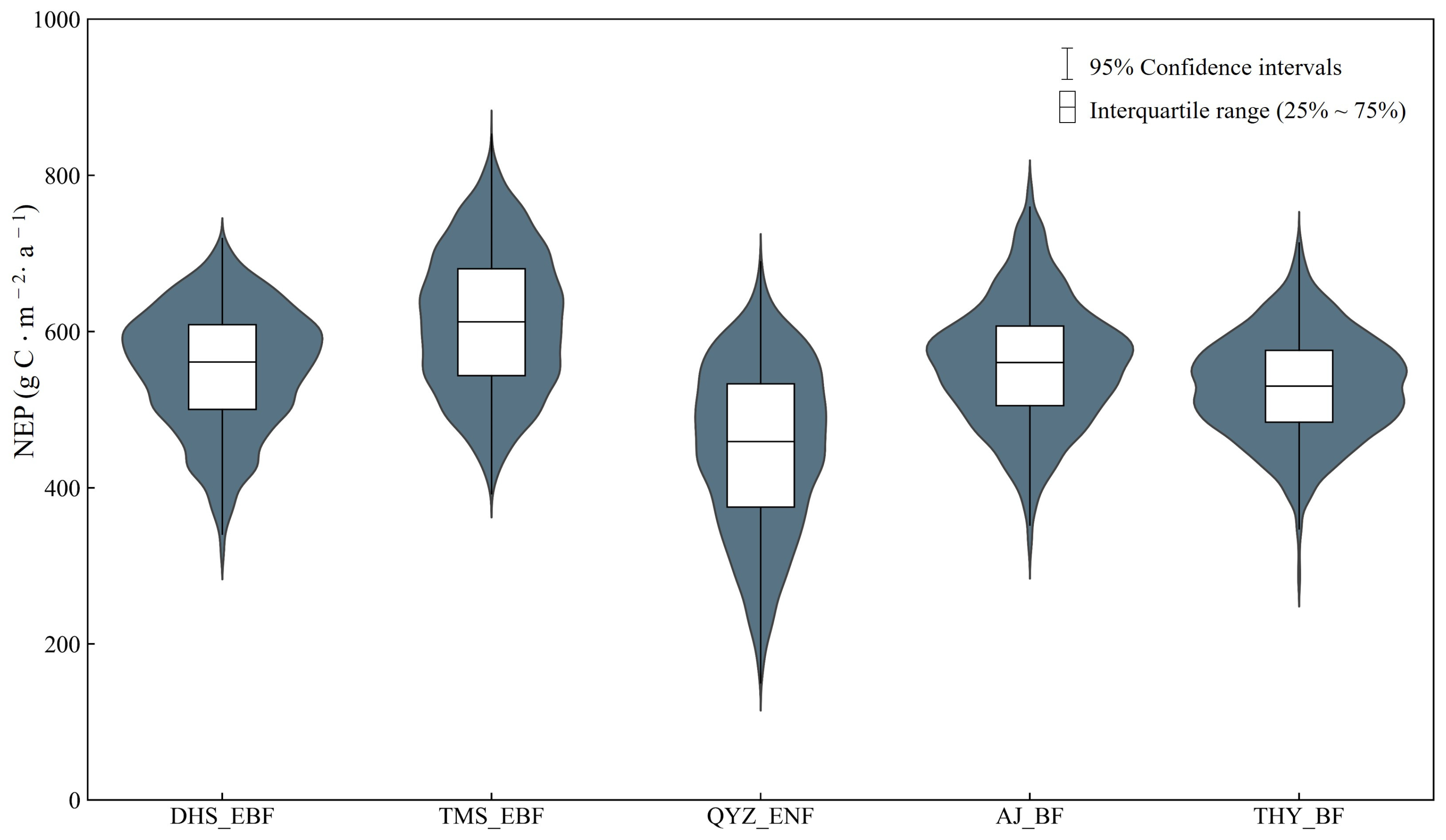
3.1. Uncertainty Analysis

The uncertainty of the input data was calculated using the EFAST, as shown in Figure 4. The EBF (DHS site) had the highest NEP values, with a distribution ranging from 392 to 852 gC∙m−2∙a−1. The ENF (QYZ site) had a relatively scattered distribution of NEP, with a range of 150 to 690 gC∙m−2∙a−1. The NEP distribution of the BF (THY site) was relatively concentrated. Table 4 shows that there was no significant difference in the coefficient of variations (CV) between the two EBF sites, with a 13.86% CV for DHS and a 14.55% CV for TMS. The uncertainty in the ENF (CV, 23.22%) was significantly higher than that of the EBF and BF (CV = 14.24% and CV = 12.78%).

3.2. Morris Sensitivity Analysis

Figure 5 shows the sensitivity indices of the physiological and ecological parameters at each of the five sites ( μ , σ ). For the EBF, k was the most influential parameter at both sites. In addition to k, the order of sensitive parameters at DHS was SLA, Gsmax, SC:LC, Q10Ract, and Gbl; for TMS, the sensitive parameters were in the order SLA, Gsmax, Gbl, FLNR, and Ract25. The order of the top three parameters was the same for both sites; however, the order of the less-sensitive parameters differed. The sensitive parameters affecting the ENF at QYZ were k, MRpern, Kc25, Q10Rac, Gbl, FLNR, and SC:LC. Additionally, k determines the amount of light energy that can be sequestered by the canopy, which directly affects the total photosynthetic primary productivity of the stand and shows high sensitivity in both the EBF and ENF. For the BF, AJ and THY were similar in terms of topography, soil, climate, and other conditions and their sensitivity parameters and rankings were also highly similar. The sensitivity parameters and rankings of AJ were Ract25 > Ko25 > Q10Rac > FLNR > FRC:LC > Kc25 > SCRages. Compared with AJ, THY had the fourth highest rank of Ko25 and the remaining sensitivities were consistent.

3.3. EFAST Sensitivity Analysis

The physiological and ecological parameters of Si and SiT for each of the five observation sites are shown in Figure 6.
For the EBF, the highly sensitive parameters affecting the NEP simulation results at DHS were k, SLA, Gsmax, and SC:LC and the moderately sensitive parameters were Gbl, Q10Ract, and FRC:LC. Among them, the SiT of k was much larger than that of Si; the SiT of Gsmax, Gbl, and Q10Ract was >0.1 and that of Si was <0.1, suggesting that these four parameters mainly influence the NEP simulated values through interaction with other parameters. The SiT of FRC:LC was <0; whereas, that of Si was >0, indicating that FRC:LC directly affects the NEP simulation results. Additionally, k was shown to be a highly sensitive parameter that affected the NEP simulation results at TMS and the moderately sensitive parameters were FLNR, Gbl, Gsmax, Ract25, C:Nleaf, and SLA. In addition, k, SLA, FLNR, and Gbl were common sensitive parameters at DHS and TMS. The EBF physiological and ecological parameters of different sites showed similar combinations of sensitive parameters.
The high-sensitivity parameters affecting the NEP simulation results at QYZ were k and MRpern and the medium-sensitivity parameters were Q10Ract, Gbl, FLNR, SC:LC, and Kc25, where the SiT of SC:LC was >0.1 and that of Si was <0.1. This suggests that SC:LC does not directly affect the results but rather varies synergistically with the other parameters, affecting the simulated NEP.
For the BF, the high-sensitivity parameters affecting the NEP simulation results at AJ were Ko25, SCRages, Ract25, and FRC:LC and the medium-sensitivity parameters included Fer, Kc25, Q10Ract, FLNR, and k. The high-sensitivity parameters affecting the NEP simulation results at THY were Ract25, Q10Ract, and SCRages and the medium-sensitivity parameters included FRC:LC, Ko25, FLNR, and Fer. The differences in the Si and the SiT of the sensitive parameters at both sites were small and they mainly affected the NEP of the BF through direct effects. Among these, SCRages and Fer are bamboo-forest-specific parameters that significantly affected the NEP simulation results for the BF.

3.4. Comparative Analysis of Morris and EFAST Results

As shown in Figure 7, the combination of the two sensitivity analysis methods led to ten key sensitive parameters affecting NEP: k, SC:LC, SLA, FRC:LC, Gsmax, MRpern, Ko25, Ract25, Q10Ract, and SCRages (for the BF only). The most sensitive parameter of the EBF and ENF calculated using the Morris method was k. The key control parameter of the BF (THY) was Ract25, which is consistent with the results of the EFAST. At DHS, the EFAST added FRC:LC over the Morris method. At TMS, C:Nleaf was added; at QYZ, the types of sensitive parameters were the same but the ordering was different. At AJ and THY, the EFAST added the bamboo-forest-specific parameter Fer over the Morris method. The types of sensitive parameters screened by the two methods that have a large impact on the NEP were highly similar; however, the order of importance of sensitive parameters was different. The EFAST generally calculates more sensitive parameters than the Morris method, partly because of the number of samples and partly due to the effects caused by the coupling of the parameters. The key control parameters vary from site to site and the key control parameters of each site show the same sensitivity at other sites with different degrees of sensitivity. Additionally, k is the common sensitive parameter in QYZ, DHS, TMS, and AJ and showed high sensitivity in the EBF (QYZ) and ENF (DHS and TMS), with a SiT of 0.4 or more, the first in the Morris method. In addition to k, MRpern was the most sensitive parameter for the ENF (QYZ) (SiT = 0.34 and μ   = 0.54), SLA was the most sensitive parameter for the EBF (DHS) (SiT = 0.39 and μ ranged from 0.65 to 0.75), and Ko25 and Ract25 were the most influential parameters for the BF (AJ and THY) (SiT = 0.48, SiT = 0.56 and μ ranged from 0.5 to 1).

3.5. BIOME-BGC Model Validation

The carbon flux values simulated by the parameter localized model are closer to the flux observations than the original model. The original model had unrealistic peaks while the accuracy was significantly improved by the parameter-localized model (Figure 8). The R of NEP simulated using the original model ranged from 0.45 to 0.66 and NRMSE ranged from 15.88 to 28.43% for the five sites; the R of NEP simulated using the parameter-optimized model ranged from 0.61 to 0.75 and NRMSE ranged from 14.83 to 21.09%. Compared with the original model, the average R of the localized model improved by 25.19% and the average NRMSE reduced by 21.74%. The localized model can better simulate the changing characteristics of carbon fluxes in subtropical forests.

4. Discussion

4.1. Uncertainty Analysis

Uncertainty in the BIOME-BGC model arises from many sources, including the model structure, input variables, and model parameters [54]. Uncertainty in the model structure may be due to an insufficient understanding of ecosystem processes and the simplification of ecological process mechanisms by modelers [55,56]. The effects of forest fires and anthropogenic activities [8], for example, on carbon and nitrogen water cycles were not considered in this simulation, which may generate uncertainty. Uncertainty in the input variables may be caused by measurement errors, insufficient data collection, or statistics [57,58]. There are two main reasons for uncertainty in the model parameters. First, some input parameters cannot be directly observed, especially those related to carbon and nitrogen ratios and partitioning. Second, obtaining a range of parameter variations is difficult (e.g., Q10kc, C:Nleaf, MRpern). For some parameters that were difficult to obtain, we reviewed the literature and directly used default model values, which may lead to uncertainty. The range of parameter values has a significant effect on the results of sensitivity analyses. A smaller baseline value is more likely to be affected by the parameter range and smaller parameter ranges limit their sensitivity indexes [59]. The wide range of variability in the NEP for the ENF indicates that when generating multiple sets of sample parameters, some combinations contained parameters that were outside the normal range of physiological parameters of the ENF (Figure 4 and Table 4), representing forests experiencing unsustainable or disturbed growth during the years simulated by the model, which led to lower NEP values in the simulations. However, sensitivity analyses are not affected by these conditions owing to the presence of available and useful spin-up phases [53]. Therefore, we controlled the parameter fluctuation amplitude to 20%, which ensured consistency in the parameter range to a certain extent.
When comparing the results of the variance-based method (e.g., EFAST) with those of the Morris method, the different forms of distribution of the input parameters can lead to uncertainties in the sensitivity indices [14,60]. When the input parameters of the models are independent of each other and obey a uniform distribution, the sensitivity indices show a high correlation. However, when the input parameters are arbitrarily distributed, the results will greatly differ between the methods and μ i will not represent SiT well [61,62]. In this study, the distribution form of the input parameters was set to be uniform, and the results showed that the types of sensitive parameters screened by the two methods were basically similar. However, there were differences in the ordering of the sensitive parameters, which was also reflected in the following studies. Ciffroy and Benedetti [63] analyzed the parameters of a geochemical morphology model using the two methods and the types of sensitive parameters calculated by the two methods were similar but the ordering was slightly different. Peng et al. [18] used the Morris method and EFAST to analyze the global sensitivity of the parameters of the DCSEM model and the sensitive parameters were similar. Xue et al. [64] applied the two methods to a process model (CROBAS model) and the sensitivity parameters were similar but with slight differences in importance. The differences between the results are, firstly, due to the different sample sizes used for the two methods (the sample size and computational volume of the EFAST are larger). Secondly, the results of the sensitivity analysis of the output variables are affected by the strength of the interactions between the parameters while the Morris method cannot judge the interaction between the parameters based on the magnitude of μ i , thus underestimating the sensitivity of some parameters. Both methods can effectively screen out the important parameters affecting the output of the model. The Morris method has a significant advantage when the sample size is small, parameters are numerous, and the time required for the model operation is long. The EFAST can further quantitatively analyze the contribution of each input parameter and the interactions between the parameters to the simulation results [18]. Therefore, for parameter sensitivity analyses of complex process models, the Morris method can be used for qualitative studies and the EFAST for quantitative evaluations.

4.2. Sensitive Parameters

Sensitivity analyses based on both the Morris method and EFAST showed that k, SC:LC, SLA, FRC:LC, Gsmax, MRpern, Ko25, Ract25, Q10Ract, and SCRages (for the BF only) significantly affected the simulated NEP. However, there may be differences in parameter sensitivity owing to forest type, growing environment, geographic location, and other factors. Liu et al. [26] analyzed the parameter sensitivity of rubber trees in Hainan Province, China, and found that the key sensitive parameter affecting the carbon flux output of the model was k, followed by SLA and C:Nleaf, with FLNR, FRC:LC, and SC:LC also showing sensitivity. Kumar and Raghubanshi [27] reported k, SLA, SC:LC, and Gsmax as highly sensitive parameters affecting carbon fluxes in dry tropical forests, with k being the most influential. Raj et al. [25] found that Douglas fir carbon fluxes in the Speulderbos forest in the Netherlands were consistently the most sensitive to FLNR, with the second most sensitive parameter being FRC:LC, followed by SC:LC and SLA. Yan et al. [23] simulated forest carbon fluxes in the Changbaishan region and showed that FLNR was the most sensitive; SLA and Gsmax also showed high sensitivity but k did not. Ritika et al. [65] reported sensitivity analyses for Indian forests and yielded similar parameters, with changes in SLA values having the greatest impact on carbon flux simulations. In general, the main physiological and ecological parameters affecting ecosystem carbon fluxes in the BIOME-BGC model were those affecting photosynthesis and respiration; however, the maximum sensitivity parameters of their respective responses differed because of the environment, vegetation type, and other factors. This is also true for the results of the present study, which illustrates the reasonableness and reliability of the results.
For the study area and forest types used in this study, k showed high sensitivity in both EBF and ENF. Additionally, k reflects the extent to which the light passing through the vegetation layer is subjected to processes, such as absorption, scattering, and reflection. When k decreases, more light passes through the vegetation layer to reach the ground, thus affecting the intensity of photosynthesis and evapotranspiration in plants and contributing to an increase in carbon fixation and net carbon balance. Conversely, when k increases, the absorption, scattering, and reflection of light by vegetation increases, allowing less light to pass through the vegetation layer to reach the ground, thus reducing carbon fixation and the net carbon balance. In addition to k, MRpern was the most sensitive parameter in the ENF; MRpern represents the coefficient of the linear relationship between tissue N and maintenance respiration and is directly related to maintenance respiration, which, in turn, affects NEP [66]. SLA was the most influential parameter in the EBF and mainly affects plant photosynthesis by influencing the area and intensity of light received by the leaves. Changes in SC:LC values affect the calculation of leaf carbon content, subsequently affecting plant growth and photosynthesis. Gsmax is an important parameter for plants to regulate gas exchange and photosynthesis. When Gsmax decreases, the concentration of CO2 in the leaf decreases, which, in turn, reduces the rate of photosynthesis [67]. Q10Ract, Ko25, and Ract25 affect the photosynthetic efficiency of leaves by controlling the levels of photosynthesis-related enzymes that influence the output of carbon flux [68]. FRC:LC is also an important parameter and when FRC:LC increases (more carbon in the leaves is transferred to the fine roots), leaf growth is inhibited, which, in turn, affects the accumulation of carbon in the plants [69]. SCRages, a bamboo-forest-specific parameter, significantly reduces the aboveground carbon stocks in bamboo forests and has a non-negligible effect on stand productivity [70,71]. Atmospheric carbon enters the biosphere through photosynthesis and returns to the atmosphere through respiration and these two physiological processes are crucial to ecosystem carbon cycles [42]. Therefore, it is reasonable to assume that the parameters affecting photosynthesis and respiration are the most sensitive to the carbon flux output of the BIOME-BGC model and the parameters affecting photosynthesis and respiration should be considered first for correction when the model is extrapolated to other regions. The results of this study clarified the key sensitive parameters of carbon fluxes in different regions and vegetation types and provided data to support the accurate simulation of carbon fluxes and the correction of model parameters at the regional scale.

5. Conclusions

The key sensitive parameters affecting NEP in subtropical forest ecosystems were explored and analyzed in the BIOME-BGC model using the Morris method and EFAST and the localized BIOME-BGC model was validated using flux observation data. The following conclusions were drawn:
  • Both the Morris method and EFAST can effectively screen out the important parameters affecting the output of the model. The Morris method has a significant advantage when the sample size is small, the parameters are numerous, and the computational effort is high; however, it is only a qualitative method of parameter sensitivity analysis. The EFAST method allows further quantitative analysis of the contribution of each input parameter and the interaction between parameters to the simulation results; however, its computational efficiency is lower than that of the Morris method. For parameter sensitivity analyses of complex process models, the Morris method is used for qualitative studies and the EFAST method is used for quantitative studies;
  • The parameters k, SC:LC, SLA, FRC:LC, Gsmax, MRpern, Ko25, Ract25, Q10Ract, and SCRages (only for the BF) significantly affected the simulated subtropical forest NEP. Priority should be given to these parameters in model parameter optimization and correction to reduce computation and improve model accuracy;
  • Compared with the flux observation data, the parameter-optimized BIOME-BGC model significantly improved the simulation ability of the original model for the NEP of subtropical forest ecosystems in China; the average R of the NEP increased by 25.19% and the average NRMSE reduced by 21.74%.
This study deepens the understanding of the process model and provides a reliable solution for accurate spatial and temporal simulations of the subtropical forest carbon cycle.

Supplementary Materials

The following supporting information can be downloaded at: https://www.mdpi.com/article/10.3390/f15030552/s1, Table S1. Photosynthesis-related parameters involved in sensitive analyses of the BIOME-BGC model. Table S2. Respiratory-related and other physio-ecological parameters involved in sensitivity analysis of BIOME-BGC model.

Author Contributions

Conceptualization, J.S.; Methodology, J.S.; Software, J.S., C.X. and F.Y.; Validation, J.S.; Formal analysis, J.S.; Investigation, J.S.; Data curation, C.X., Z.Z., X.T., F.Y., N.Y. and Z.H.; Writing—original draft, J.S.; Writing—review & editing, F.M.; Supervision, F.M., H.D. and X.L. All authors have read and agreed to the published version of the manuscript.

Funding

The authors gratefully acknowledge the support of the Leading Goose Project of the Science Technology Department of Zhejiang Province (No. 2023C02035), National Natural Science Foundation of China (No. 32171785, 32201553, 31901310), Scientific Research Project of Baishanzu National Park (No. 2022JBGS02).

Data Availability Statement

The data presented in this study are available on request from the corresponding author.

Conflicts of Interest

The authors declare no conflict of interest.

References

  1. Buotte, P.C.; Law, B.E.; Ripple, W.J.; Berner, L.T. Carbon sequestration and biodiversity co-benefits of preserving forests in the western United States. Ecol. Appl. 2020, 30, e02039. [Google Scholar] [CrossRef]
  2. Mcveigh, P.; Sottocornola, M.; Foley, N.; Leahy, P.; Kiely, G. Meteorological and functional response partitioning to explain interannual variability of CO2 exchange at an Irish Atlantic blanket bog. Agric. For. Meteorol. 2014, 194, 8–19. [Google Scholar] [CrossRef]
  3. Mao, F.; Du, H.; Zhou, G.; Zheng, J.; Li, X.; Xu, Y.; Huang, Z.; Yin, S. Simulated net ecosystem productivity of subtropical forests and its response to climate change in Zhejiang Province, China. Sci. Total Environ. 2022, 838, 155993. [Google Scholar] [CrossRef]
  4. Mitchard, E.T.A. The tropical forest carbon cycle and climate change. Nature 2018, 559, 527–534. [Google Scholar] [CrossRef] [PubMed]
  5. Fennel, K.; Losch, M.; Schröter, J.; Wenzel, M. Testing a marine ecosystem model: Sensitivity analysis and parameter optimization. J. Mar. Syst. 2001, 28, 45–63. [Google Scholar] [CrossRef]
  6. Raj, R.; Tol, C.V.D.; Hamm, N.A.S.; Stein, A. Bayesian integration of flux tower data into a process-based simulator for quantifying uncertainty in simulated output. Geosci. Model Dev. 2016, 11, 83–101. [Google Scholar] [CrossRef]
  7. He, L.H.; Wang, H.Y.; Lei, X.D. Parameter sensitivity of simulating net primary productivity of Larix olgensis forest based on BIOME-BGC model. Chin. J. Appl. Ecol. 2016, 27, 412–420. [Google Scholar]
  8. Du, L.; Zeng, Y.; Ma, L.; Qiao, C.; Wu, H.; Su, Z.; Bao, G. Effects of anthropogenic revegetation on the water and carbon cycles of a desert steppe ecosystem. Agric. For. Meteorol. 2021, 300, 108339. [Google Scholar] [CrossRef]
  9. Tian, X.; Yan, M.; Van Der Tol, C.; Li, Z.; Su, Z.; Chen, E.; Li, X.; Li, L.; Wang, X.; Pan, X.; et al. Modeling forest above-ground biomass dynamics using multi-source data and incorporated models: A case study over the qilian mountains. Agric. For. Meteorol. 2017, 246, 1–14. [Google Scholar] [CrossRef]
  10. Keller, E.D.; Baisden, W.T.; Timar, L.; Mullan, B.; Clark, A. Grassland production under global change scenarios for New Zealand pastoral agriculture. Geosci. Model Dev. 2014, 7, 2359–2391. [Google Scholar] [CrossRef]
  11. Saltelli, A.; Annoni, P. How to avoid a perfunctory sensitivity analysis. Environ. Modell. Softw. 2010, 25, 1508–1517. [Google Scholar] [CrossRef]
  12. Cukier, R.; Levine, H.; Shuler, K. Nonlinear sensitivity analysis of multiparameter model systems. J. Comput. Phys. 1978, 26, 1–42. [Google Scholar] [CrossRef]
  13. Morris, M.D. Factorial Sampling Plans for Preliminary Computational Experiments. Technometrics 1991, 33, 161–174. [Google Scholar] [CrossRef]
  14. Sobol, I.M. Global sensitivity indices for nonlinear mathematical models and their Monte Carlo estimates. Math. Comput. Simul. 2001, 55, 271–280. [Google Scholar] [CrossRef]
  15. Saltelli, A.; Tarantola, S.; Chan, K.P.S. A Quantitative Model-Independent Method for Global Sensitivity Analysis of Model Output. Technometrics 1999, 41, 39–56. [Google Scholar] [CrossRef]
  16. Wang, S.; Flipo, N.; Romary, T. Time-dependent global sensitivity analysis of the C-RIVE biogeochemical model in contrasted hydrological and trophic contexts. Water Res. 2018, 144, 341–355. [Google Scholar] [CrossRef] [PubMed]
  17. Dejonge, K.C.; Ascough Ii, J.C.; Ahmadi, M.; Andales, A.A.; Arabi, M. Global sensitivity and uncertainty analysis of a dynamic agroecosystem model under different irrigation treatments. Ecol. Model. 2012, 231, 113–125. [Google Scholar] [CrossRef]
  18. Peng, X.; Adamowski, J.; Inam, A.; Alizadeh, M.R.; Albano, R. Development of a behaviour-pattern based global sensitivity analysis procedure for coupled socioeconomic and environmental models. J. Hydrol. 2020, 585, 124745. [Google Scholar] [CrossRef]
  19. Li, Z.; Jin, X.; Liu, H.; Xu, X.; Wang, J. Global sensitivity analysis of wheat grain yield and quality and the related process variables from the DSSAT-CERES model based on the extended Fourier Amplitude Sensitivity Test method. J. Integr. Agric. 2019, 18, 1547–1561. [Google Scholar] [CrossRef]
  20. Gilardelli, C.; Confalonieri, R.; Cappelli, G.A.; Bellocchi, G. Sensitivity of WOFOST-based modelling solutions to crop parameters under climate change. Ecol. Model. 2018, 368, 1–14. [Google Scholar] [CrossRef]
  21. Li, L.; Wei, S.; Lian, J.; Cao, H. Distributional regularity of species diversity in plant community at different latitudes in subtropics. Chin. J. Ecol. 2020, 40, 1249–1257. [Google Scholar]
  22. Yuen, J.Q.; Fung, T.; Ziegler, A.D. Carbon stocks in bamboo ecosystems worldwide: Estimates and uncertainties. For. Ecol. Manag. 2017, 393, 113–138. [Google Scholar] [CrossRef]
  23. Yan, M.; Tian, X.; Li, Z.; Chen, E.; Wang, X.; Han, Z.; Sun, H. Simulation of Forest Carbon Fluxes Using Model Incorporation and Data Assimilation. Remote Sens. 2016, 8, 567. [Google Scholar] [CrossRef]
  24. Tatarinov, F.A.; Cienciala, E. Application of BIOME-BGC model to managed forests: 1. Sensitivity analysis. For. Ecol. Manag. 2006, 237, 267–279. [Google Scholar] [CrossRef]
  25. Raj, R.; Hamm, N.a.S.; Van Der Tol, C.; Stein, A. Variance-based sensitivity analysis of BIOME-BGC for gross and net primary production. Ecol. Model. 2014, 292, 26–36. [Google Scholar] [CrossRef]
  26. Liu, J.; Wu, Z.; Yang, S.; Yang, C. Sensitivity Analysis of Biome-BGC for Gross Primary Production of a Rubber Plantation Ecosystem: A Case Study of Hainan Island, China. Int. J. Environ. Res. Public Health 2022, 19, 14068. [Google Scholar] [CrossRef]
  27. Kumar, M.; Raghubanshi, A.S. Sensitivity analysis of BIOME-BGC model for dry tropical forests of Vindhyan highlands, India. Remote Sens. Spat. Inf. Sci. 2012, 38, 129–133. [Google Scholar] [CrossRef]
  28. Mao, F.; Du, H.; Zhou, G.; Li, X.; Xu, X.; Li, P.; Sun, S. Coupled LAI assimilation and BEPS model for analyzing the spatiotemporal pattern and heterogeneity of carbon fluxes of the bamboo forest in Zhejiang Province, China. Agric. For. Meteorol. 2017, 242, 96–108. [Google Scholar] [CrossRef]
  29. Papale, D.; Reichstein, M.; Aubinet, M.; Canfora, E.; Bernhofer, C.; Kutsch, W.; Longdoz, B.; Rambal, S.; Valentini, R.; Vesala, T. Towards a standardized processing of Net Ecosystem Exchange measured with eddy covariance technique: Algorithms and uncertainty estimation. Biogeosciences 2006, 3, 571–583. [Google Scholar] [CrossRef]
  30. Lasslop, G.; Reichstein, M.; Papale, D.; Richardson, A.D.; Arneth, A.; Barr, A.; Stoy, P.; Wohlfahrt, G. Separation of net ecosystem exchange into assimilation and respiration using a light response curve approach: Critical issues and global evaluation. Glob. Change Biol. 2010, 16, 187–208. [Google Scholar] [CrossRef]
  31. Reichstein, M.; Falge, E.; Baldocchi, D.; Papale, D.; Aubinet, M.; Berbigier, P.; Bernhofer, C.; Buchmann, N.; Gilmanov, T.; Granier, A. On the separation of net ecosystem exchange into assimilation and ecosystem respiration: Review and improved algorithm. Glob. Change Biol. 2005, 11, 1424–1439. [Google Scholar] [CrossRef]
  32. Fujisada, H.; Bailey, G.B.; Kelly, G.G.; Hara, S.; Abrams, M.J. Aster dem performance. IEEE Trans. Geosci. Remote Sens. 2005, 43, 2707–2714. [Google Scholar] [CrossRef]
  33. Running, S.W.; Coughlan, J.C. A general model of forest ecosystem processes for regional applications I. Hydrologic balance, canopy gas exchange and primary production processes. Ecol. Model. 1988, 42, 125–154. [Google Scholar] [CrossRef]
  34. Running, S.W.; Hunt, E.R., Jr. Generalization of a Forest Ecosystem Process Model for other Biomes, BIOME-BCG, and an Application for Global-Scale Models; Academic Press: Cambridge, MA, USA, 1993. [Google Scholar]
  35. Du, H.; Mao, F.; Zhou, G.; Li, X.; Xu, X.; Ge, H.; Cui, L.; Liu, Y.; Zhu, D.E.; Li, Y. Estimating and Analyzing the Spatiotemporal Pattern of Aboveground Carbon in Bamboo Forest by Combining Remote Sensing Data and Improved BIOME-BGC Model. IEEE J. Sel. Top. App. Earth Observ. Remote Sens. 2018, 11, 2282–2295. [Google Scholar] [CrossRef]
  36. Mao, F.; Li, P.; Zhou, G.; Du, H.; Xu, X.; Shi, Y.; Mo, L.; Zhou, Y.; Tu, G. Development of the BIOME-BGC model for the simulation of managed Moso bamboo forest ecosystems. J. Environ. Manag. 2016, 172, 29–39. [Google Scholar] [CrossRef] [PubMed]
  37. Thornton, P.E.; Rosenbloom, N.A. Ecosystem model spin-up: Estimating steady state conditions in a coupled terrestrial carbon and nitrogen cycle model. Ecol. Model. 2005, 189, 25–48. [Google Scholar] [CrossRef]
  38. Thornton, P.E.; Law, B.E.; Gholz, H.L.; Clark, K.L.; Falge, E.; Ellsworth, D.S.; Goldstein, A.H.; Monson, R.K.; Hollinger, D.; Falk, M. Modeling and measuring the effects of disturbance history and climate on carbon and water budgets in evergreen needleleaf forests. Agric. For. Meteorol. 2002, 113, 185–222. [Google Scholar] [CrossRef]
  39. Campolongo, F.; Cariboni, J.; Saltelli, A. An effective screening design for sensitivity analysis of large models. Environ. Modell. Softw. 2007, 22, 1509–1518. [Google Scholar] [CrossRef]
  40. Saltelli, A.; Ratto, M.; Andres, T.; Campolongo, F.; Cariboni, J.; Gatelli, D.; Saisana, M.; Tarantola, S. Global Sensitivity Analysis: The Primer; John Wiley & Sons: Chichester, UK, 2008. [Google Scholar]
  41. White, M.A.; Thornton, P.E.; Running, S.W.; Nemani, R.R. Parameterization and Sensitivity Analysis of the BIOME–BGC Terrestrial Ecosystem Model: Net Primary Production Controls. Earth Interact. 2000, 4, 1–85. [Google Scholar] [CrossRef]
  42. Waring, R.H.; Running, S.W. Forest Ecosystems: Analysis at Multiple Scales; Elsevier: Amsterdam, The Netherlands, 2010. [Google Scholar]
  43. Woodrow, I.E.; Berry, J.A. Enzymatic Regulation of Photosynthetic CO2, Fixation in C3 Plants. Annu. Rev. Plant Physiol. Plant Molec. Biol. 1988, 39, 533–594. [Google Scholar] [CrossRef]
  44. Wu, Y.; Wang, X.; Ouyang, S.; Xu, K.; Hawkins, B.A.; Sun, O.J. A test of BIOME-BGC with dendrochronology for forests along the altitudinal gradient of Mt. Changbai in northeast China. J. Plant Ecol. 2016, 123, 439–452. [Google Scholar] [CrossRef]
  45. Zhou, C.-H.; Hao, Z.-Q.; He, H.-S.; Zhou, D.-H. Sensitivity of parameters in net primary productivity model of broadleaf-Korean pine mixed forest. Chin. J. Appl. Ecol. 2008, 19, 929–935. [Google Scholar]
  46. Gao, Q.; Peng, S.; Zhao, P.; Zeng, X.; Cai, X.; Yu, M.; Shen, W.; Liu, Y. Explanation of vegetation succession in subtropical southern China based on ecophysiological characteristics of plant species. Tree Physiol. 2003, 23, 641–648. [Google Scholar] [CrossRef]
  47. Lu, W.; Fan, W.Y.; Tian, T. Parameter optimization of BEPS model based on the flux data of the temperate deciduous broad-leaved forest in Northeast China. Chin. J. Appl. Ecol. 2016, 27, 1353–1358. [Google Scholar]
  48. Liu, G.; Fan, S.; Su, W.; Xiao, F.; Huang, Y. Distribution Characteristics and Coupling Relationship of Organic Carbon and Total Nitrogen in Phyllostachys pubescens Forests with Different Operations and Management Modes. J. Soil Water Conserv. 2010, 24, 218–222. [Google Scholar]
  49. Zhang, J.; Zhang, D.; Jian, Z.; Zhou, H.; Zhao, Y.; Wei, D. Litter decomposition and the degradation of recalcitrant components in Pinus massoniana plantations with various canopy densities. J. For. Res. 2019, 30, 1395–1405. [Google Scholar] [CrossRef]
  50. Liu, Z.; Fei, B. Characteristics of Moso Bamboo with Chemical Pretreatment; IntechOpen: London, UK, 2013. [Google Scholar]
  51. Holling, C.S.; Schindler, D.W.; Walker, B.H.; Roughgarden, J. Biodiversity in the Functioning of Ecosystems: An Ecological Synthesis; Cambridge University Press: Cambridge, UK, 1995. [Google Scholar]
  52. Jin, A. High Profit Management and Participatory Development of Phyllostachys Pubescens Plantation in Zhejiang and Fujian Mountainous Areas. Ph.D. Dissertation, Nanjing Forestry University, Nanjing, China, 2004. [Google Scholar]
  53. Ren, H.; Zhang, L.; Yan, M.; Tian, X.; Zheng, X. Sensitivity analysis of Biome-BGCMuSo for gross and net primary productivity of typical forests in China. For. Ecosyst. 2022, 9, 100011. [Google Scholar] [CrossRef]
  54. Li, X.; Sun, J. Testing parameter sensitivities and uncertainty analysis of Biome-BGC model in simulating carbon and water fluxes in broadleaved-Korean pine forests. Chin. J. Plant Ecol. 2018, 42, 1131–1144. [Google Scholar] [CrossRef]
  55. Kang, M. Energy Partitioning and Modelling of Carbon and Water fluxes of a Poplar Plantation Ecosystem in Northern China. Ph.D. Dissertation, Beijing Forestry University, Beijing, China, 2016. [Google Scholar]
  56. Zheng, L.; Song, S.; Yuan, X.; Dong, J.; Li, L. Simulation of water and carbon fluxes in a broad-leaved Korean pine forest in Changbai Mountains based on Biome-BGC model and Ensemble Kalman Filter method. Chin. J. Ecol. 2017, 36, 1752–1760. [Google Scholar]
  57. Jung, M.; Vetter, M.; Herold, M.; Churkina, G.; Reichstein, M.; Zaehle, S.; Ciais, P.; Viovy, N.; Bondeau, A.; Chen, Y. Uncertainties of modeling gross primary productivity over Europe: A systematic study on the effects of using different drivers and terrestrial biosphere models. Glob. Biogeochem. Cycle. 2007, 21. [Google Scholar] [CrossRef]
  58. Eastaugh, C.S.; Pötzelsberger, E.; Hasenauer, H. Assessing the impacts of climate change and nitrogen deposition on Norway spruce (Picea abies L. Karst) growth in Austria with BIOME-BGC. Tree Physiol. 2011, 31, 262–274. [Google Scholar]
  59. Ma, H.; Ma, C.; Li, X.; Yuan, W.; Liu, Z.; Zhu, G. Sensitivity and uncertainty analyses of flux-based ecosystem model towards improvement of forest GPP simulation. Sustainability 2020, 12, 2584. [Google Scholar] [CrossRef]
  60. Saltelli, A.; Annoni, P.; Azzini, I.; Campolongo, F.; Ratto, M.; Tarantola, S. Variance based sensitivity analysis of model output. Design and estimator for the total sensitivity index. Comput. Phys. Commun. 2010, 181, 259–270. [Google Scholar] [CrossRef]
  61. Feng, K.; Lu, Z.; Yang, C. Enhanced Morris method for global sensitivity analysis: Good proxy of Sobol’ index. Struct. Multidiscip. Optim. 2018, 59, 373–387. [Google Scholar] [CrossRef]
  62. Sobol, I.; Kucherenko, S. Derivative based global sensitivity measures. Procedia. Soc. Behav. Sci. 2010, 2, 7745–7746. [Google Scholar] [CrossRef]
  63. Ciffroy, P.; Benedetti, M. A comprehensive probabilistic approach for integrating natural variability and parametric uncertainty in the prediction of trace metals speciation in surface waters. Environ. Pollut. 2018, 242, 1087–1097. [Google Scholar] [CrossRef]
  64. Xue, H.; Tian, X.; Wang, B.; Sun, S.; Cao, T. Comparison of global sensitivity analysis techniques based on a process-based model CROBAS. Chin. J. Appl. Ecol. 2021, 32, 134–144. [Google Scholar]
  65. Srinet, R.; Nandy, S.; Patel, N.R.; Padalia, H.; Watham, T.; Singh, S.K.; Chauhan, P. Simulation of forest carbon fluxes by integrating remote sensing data into biome-BGC model. Ecol. Model. 2023, 475, 110185. [Google Scholar] [CrossRef]
  66. Ryan, M.G. Effects of climate change on plant respiration. Ecol. Appl. 1991, 1, 157–167. [Google Scholar] [CrossRef]
  67. Flexas, J.; Bota, J.; Escalona, J.M.; Sampol, B.; Medrano, H. Effects of drought on photosynthesis in grapevines under field conditions: An evaluation of stomatal and mesophyll limitations. Funct. Plant Biol. 2002, 29, 461–471. [Google Scholar] [CrossRef]
  68. Aber, J.D.; Federer, C.A. A generalized, lumped-parameter model of photosynthesis, evapotranspiration and net primary production in temperate and boreal forest ecosystems. Oecologia 1992, 92, 463–474. [Google Scholar] [CrossRef] [PubMed]
  69. Wang, X.; Ma, L.; Jia, Z.; Jia, L. Root inclusion net method: Novel approach to determine fine root production and turnover in Larix principis-rupprechtii Mayr plantation in North China. Turk. J. Agric. For. 2014, 38, 388–398. [Google Scholar] [CrossRef]
  70. Zhu, J.; Huang, M.; Chen, Y.; Huang, R.; Li, X. The structure of a culm and shoot producing stand of Phyllostachys pubescens. Chin. J. Plant Ecol. 2000, 24, 483. [Google Scholar]
  71. Zhang, C.; Ding, X. Analysis and Research on the Factors Affecting the Growth of Phyllostachys edulis Forest. J. Bamboo Res. 1997, 16, 31–36. [Google Scholar]
Figure 1. Typical subtropical forest distribution and the flux observation sites in China.
Forests 15 00552 g001
Figure 3. Flow chart for sensitivity analysis.
Forests 15 00552 g003
Figure 4. Distribution ranges, 95% confidence intervals, and interquartile ranges of mean annual NEP for the three forest types at the five sites.
Forests 15 00552 g004
Figure 5. Sensitivity index (μ*) and interaction index between parameters (σ) for Morris method sensitivity analyses at each site: (a) DHS site; (b) TMS site; (c) QYZ site; (d) AJ site; (e) THY site.
Forests 15 00552 g005
Figure 6. First-order sensitivity index (Si) and total-order sensitivity index (SiT) for EFAST method sensitivity analyses at each site. Sensitive and highly sensitive parameters are shown above the red dashed and solid lines, respectively.
Forests 15 00552 g006
Figure 7. Impact of key sensitive parameters screened in each site by combining the results of the EFAST method and Morris method analyses: (a) SiT of the EFAST method (SiT > 0.1 is a sensitive parameter); (b) μ* of the normalized Morris method (μ* > 0.2 is a sensitive parameter, μ* reflects only the relative magnitude of the sensitivity of the parameter and can only be used to judge the relative magnitude of the sensitivity, and its value does not reflect the true sensitivity of the parameter).
Forests 15 00552 g007
Figure 8. Comparison of the flux tower data with the corresponding simulation results using the original and optimized models. (a) DHS site; (b) TMS site; (c) QYZ site; (d) AJ site; (e) THY site.
Forests 15 00552 g008
Table 1. Information of five flux sites used in this study; the three typical forests include the evergreen broadleaf forest (EBF), evergreen needleleaf forest (ENF), and bamboo forest (BF).
Site NameLat (°N)Lon (°E)Plant Functional Type
Dinghushan (DHS)23.17112.53EBF
Tianmushan (TMS)30.32119.48EBF
Qianyanzhou (QYZ)26.74115.06ENF
Anji (AJ)30.28119.40BF
Taihuyuan (THY)30.26119.59BF
Table 2. Photosynthesis-related parameters involved in sensitive analyses of the BIOME-BGC model.
SymbolDescriptionUnit
Photosynthesis biophysics parameters
FLNRFraction of leaf N in RubiscokgNRub·kgNleaf−1
Ko25Michaelis constant of oxidation reaction at 25 °C-
Ract25Rubisco activity at 25 °Cμmol·mg·Rubisco−1·min−1
Kc25Michaelis constant of carboxylation reaction at 25 °C-
Q10kcThe Q10 temperature coefficient of kc-
Q10koThe Q10 temperature coefficient of ko-
Q10RactThe Q10 temperature coefficient of Rubisco-
Allocation of carbon parameters
FRC:LCNew fine root C: leaf CkgC·kgC−1
LWC:TWCNew live wood C: total wood CkgC·kgC−1
SC:LCNew stem C: new leaf CkgC·kgC−1
CRS:SCNew coarse root C: stem CkgC·kgC−1
CGPCurrent growth proportion-
Canopy structure biophysics parameters
WintWater interception coefficientLAI−1·d−1
kLight extinction coefficient-
SLAAverage specific leaf aream·kgC−1
SLAshd:sunRatio of shade SLA: sunlit SLA-
LAIall:projRatio of all sides to projected leaf area-
Stomatal conductance biophysics parameters
GsmaxMaximum stomatal conductancem·s−1
GblBoundary layer conductancem·s−1
LWPfLeaf water potential: completion of gs reductionMPa
LWPiLeaf water potential: start of gs reductionMPa
VPDfVapor pressure deficit: completion of gs reductionPa
VPDiVapor pressure deficit: start of gs reductionPa
GcutCuticular conductancem·s−1
Table 3. Respiratory-related and other physio-ecological parameters involved in sensitivity analysis of the BIOME-BGC model.
SymbolDescriptionUnit
Heterotrophic respiration biophysics parameters
C:NlitterC: N of falling leaf litterkgC·kgN−1
LFGLitterfall period-
LWTAnnual live wood turnover fractiona−1
Maintenance respiration biophysics parameters
MRpernMaintenance respiration in
kg C/day per kg of tissue N
kgC·kgN−1·d−1
C:NleafC: N of leaveskgC·kgN−1
C:NfrC: N of fine rootskgC·kgN−1
C:NdwC: N of dead woodkgC·kgN−1
C:NlwC: N of live woodkgC·kgN−1
Vegetation chemical parameters
TtTransfer growth period-
LlabLeaf litter labile proportion-
LligLeaf litter lignin proportion-
FRlabFine root labile proportion-
FRligFine root lignin proportion-
DWligDead wood lignin proportion-
Management measure parameters
PdswExcavation percentage of winter bamboo shoots%
Pobtr_totalThe ratio of hook tip carbon storage to total leaf carbon storage%
SCRagesSelective cutting ratio of each age-
FerApply fertilizerkgN·hm−2
PdssPercentage of bamboo shoots harvested%
Table 4. Statistical information of the annual average NEP for three forest types at five sites.
StatisticsDHS-EBFTMS-EBFQYZ-ENFAJ-BFTHY-BF
Mean551.90612.79449.89558.19529.23
Standard deviation76.4789.15104.4679.4767.65
Coefficient of variation (%) 13.8614.5523.2214.2412.78
Disclaimer/Publisher’s Note: The statements, opinions and data contained in all publications are solely those of the individual author(s) and contributor(s) and not of MDPI and/or the editor(s). MDPI and/or the editor(s) disclaim responsibility for any injury to people or property resulting from any ideas, methods, instructions or products referred to in the content.

