Article

Forest Canopy Fuel Loads Mapping Using Unmanned Aerial Vehicle High-Resolution Red, Green, Blue and Multispectral Imagery

by
Álvaro Agustín Chávez-Durán
1,2,
Mariano García
1,*,
Miguel Olvera-Vargas
2,
Inmaculada Aguado
1,
Blanca Lorena Figueroa-Rangel
2,
Ramón Trucíos-Caciano
3 and
Ernesto Alonso Rubio-Camacho
4
1
Universidad de Alcalá, Departamento de Geología, Geografía y Medio Ambiente, Environmental Remote Sensing Research Group, Calle Colegios 2, 28801 Alcalá de Henares, Spain
2
Centro Universitario de la Costa Sur, Universidad de Guadalajara, Avenida Independencia Nacional 151, Autlán de Navarro 48900, Jalisco, Mexico
3
Centro Nacional de Investigación Disciplinaria en Relación Agua, Suelo, Planta, Atmósfera, Instituto Nacional de Investigaciones Forestales, Agrícolas y Pecuarias, Margen derecho del canal del Sacramento km 6.5, Gómez Palacio 35079, Durango, Mexico
4
Campo Experimental Centro Altos de Jalisco, Centro de Investigación Regional Pacífico Centro, Instituto Nacional de Investigaciones Forestales, Agrícolas y Pecuarias, Av. Biodiversidad 2470, Tepatitlán de Morelos 47600, Jalisco, Mexico
*
Author to whom correspondence should be addressed.
Forests 2024, 15(2), 225; https://doi.org/10.3390/f15020225
Submission received: 20 December 2023 / Revised: 14 January 2024 / Accepted: 15 January 2024 / Published: 24 January 2024
(This article belongs to the Topic Application of Remote Sensing in Forest Fire)

Abstract

:
Canopy fuels determine the characteristics of the entire complex of forest fuels due to their constant changes triggered by the environment; therefore, the development of appropriate strategies for fire management and fire risk reduction requires an accurate description of canopy forest fuels. This paper presents a method for mapping the spatial distribution of canopy fuel loads (CFLs) in alignment with their natural variability and three-dimensional spatial distribution. The approach leverages an object-based machine learning framework with UAV multispectral data and photogrammetric point clouds. The proposed method was developed in the mixed forest of the natural protected area of “Sierra de Quila”, Jalisco, Mexico. Structural variables derived from photogrammetric point clouds, along with spectral information, were used in an object-based Random Forest model to accurately estimate CFLs, yielding R2 = 0.75, RMSE = 1.78 Mg, and an average B i a s r e l = 18.62%. Canopy volume was the most significant explanatory variable, achieving a mean decrease in impurity values greater than 80%, while the combination of texture and vegetation indices presented importance values close to 20%. Our modelling approach enables the accurate estimation of CFLs, accounting for the ecological context that governs their dynamics and spatial variability. The high precision achieved, at a relatively low cost, encourages constant updating of forest fuels maps to enable researchers and forest managers to streamline decision making on fuel and forest fire management.

1. Introduction

Forest fires play a crucial role in ecological disturbances in environments covered by vegetation, serving as natural shapers of forest ecosystems [1]. Three basic elements are required for a forest fire to occur: an ignition agent, oxygen, and forest fuels. Forest fuels encompass materials that have the potential to burn when exposed to an ignition source and consist of both dead organic matter and living vegetation [2]. According to the United States Department of Agriculture [3], forest fuel components can be grouped as ground (duff), surface (litter, herb, woody, and biomass within 2 m above ground), and canopy fuels (shrub, trees, and biomass above the surface). Forest fuel components are spatially distributed in three dimensions based on their inherent spatial variability and they are rarely correlated. Moreover, these components dynamically interact with the environment through complex biophysical processes [2]. Therefore, the necessity for accurate and updated fuel load maps becomes imperative for effective forest fuel management, demanding periodic measurements incurring high economic costs.
Wildfires are classified into three categories: ground, surface, and crown fires [4]. A crown fire is characterized as a fire typically initiated by a surface fire that ascends into the forest canopy, spreading through it. This type of fire proves challenging to control, often leading to catastrophic effects and demanding human intervention [5]. Reducing crown fire risk requires accurate description of canopy fuel loads (CFLs). Moreover, canopy fuels exert a significant influence on the characteristics of other fuel layers as they undergo constant changes, depending on the environment, weather, disturbances, and vegetation phenology. These factors condition fuels’ production, deposition, and decomposition [2]. Thus, CFLs synthesize many tree characteristics in an area with load, i.e., biomass, as its main indicator [6,7].
Recently, fire behavior models have included crown fire behavior predictions, allowing forest managers to make accurate decisions. Predictions are formulated to provide guidance for operational fire prevention and suppression responses, with a focus on prioritizing areas for hazardous fuel reduction management [8]. Several studies around the world have estimated CFLs, mainly through field measurements [9].
Thus, the estimation of CFLs is often conducted through field measurements, which are known to be highly expensive, time consuming, and labor intensive. Consequently, the literature frequently refers to the use of small sampling plots with limited re-measurements [10]. This approach is also difficult to apply in large areas and errors caused by human conditions tend to increase [11]. Prichard et al. (2019) [12] suggest plot-size units within the range of 0.04 to 0.10 ha to characterize and classify forest fuels, while Chávez-Durán et al. (2014) [13] and Ortíz-Mendoza et al. (2017) [14] have used plots of 0.05 ha. However, the small size of the plots did hamper the accurate estimation of CFLs, producing errors due to edge effects and the limited capacity to capture landscape variability [15].
Remote sensing offers a sound alternative to complement field measurements, especially over large and remote areas. The integration of spaceborne remote sensing with field inventory data has prompted the development of several techniques for estimating CFLs [16]. Multispectral passive satellite images have been demonstrated to be an effective and accessible tool. Passive sensors detect energy emitted or reflected from the objects and the environment. However, their primary limitation lies in their restricted sensitivity to forest structures, including fuel load, attributed to saturation at relatively low biomass levels. Active sensors provide their own source of energy to observe objects and are better suited for CFL estimation due to their higher sensitivity in capturing forest structures. In particular, Light Detection and Ranging (LiDAR) technology captures the vertical structure of forest data, allowing sharp precision and three-dimensional model generation [17]. Several studies have shown the suitability of LiDAR data to estimate canopy fuel properties from different platforms including terrestrial systems [18] and airborne [17] and spaceborne applications [19].
Several studies have proved the potential of combining active and passive remote sensors for the estimation of CFLs. Jiang et al. (2022) [20] used LiDAR and Sentinel-2 images with different Machine Learning techniques. Moran et al. (2020) [21] combined LiDAR data with Landsat through the Gradient Boosting Machine technique. García et al. (2017) [17] combined airborne LiDAR and Landsat OLI Data to extrapolate forest canopy fuel properties using Least-Squares Support Vector Machine techniques. A drawback associated with the previous studies is their coarse resolution. The spatial coverage of field plots corresponds to either a single pixel or a fraction, making it impractical to precisely estimate the variability within each plot [22]. Moreover, the overall variance tends to decrease as the pixel size increases, resulting in elevated determination coefficients that do not represent high fuel variability in the field [23].
Technological advances have paved the way for the emergence of platforms capable of transporting multiple types of sensors. LiDAR sensors have been attached to multiple airborne platforms, including conventional aircrafts and, recently, to Unmanned Aerial Vehicles (UAVs) [24]. Nevertheless, despite LiDAR’s advantages, its utilization remains expensive and the availability of UAV LiDAR sensors is still low. Instead, several algorithms have recently been developed to process conventional Red, Green, Blue (RGB) images through digital photogrammetry techniques for three-dimensional point clouds generation [25]. Furthermore, UAVs can carry sensors, allowing the acquisition of high spatial resolution images, temporal flexibility, and reliability [26].
Current advances in data collection equipment, processing techniques, and computing capability enable the development of novel methods for forest fuel management [27]. Moreover, data from diverse remote sensors as UAV high-resolution RGB and multispectral imagery, combined with field measurements and artificial intelligence techniques, are promising elements for appropriate the monitoring and management of forest fuels. Here, we present a novel approach: a cost-effective and easily replicable method which enables the monitoring of CFLs.
The aim of this paper was to devise a method for mapping the spatial distribution of CFLs in mixed forests. This was achieved by geospatial data: UAV RGB and multispectral imagery. The working hypothesis proposed that the devised method enables the consistent mapping of CFLs, considering their variability and three-dimensional spatial distribution. The results of this study offer several advantages, including optimizing time and costs involved in CFL assessment compared to traditional fieldwork. This approach enables researchers and forest managers to expedite decision-making processes for forest fire and fuel management.

2. Materials and Methods
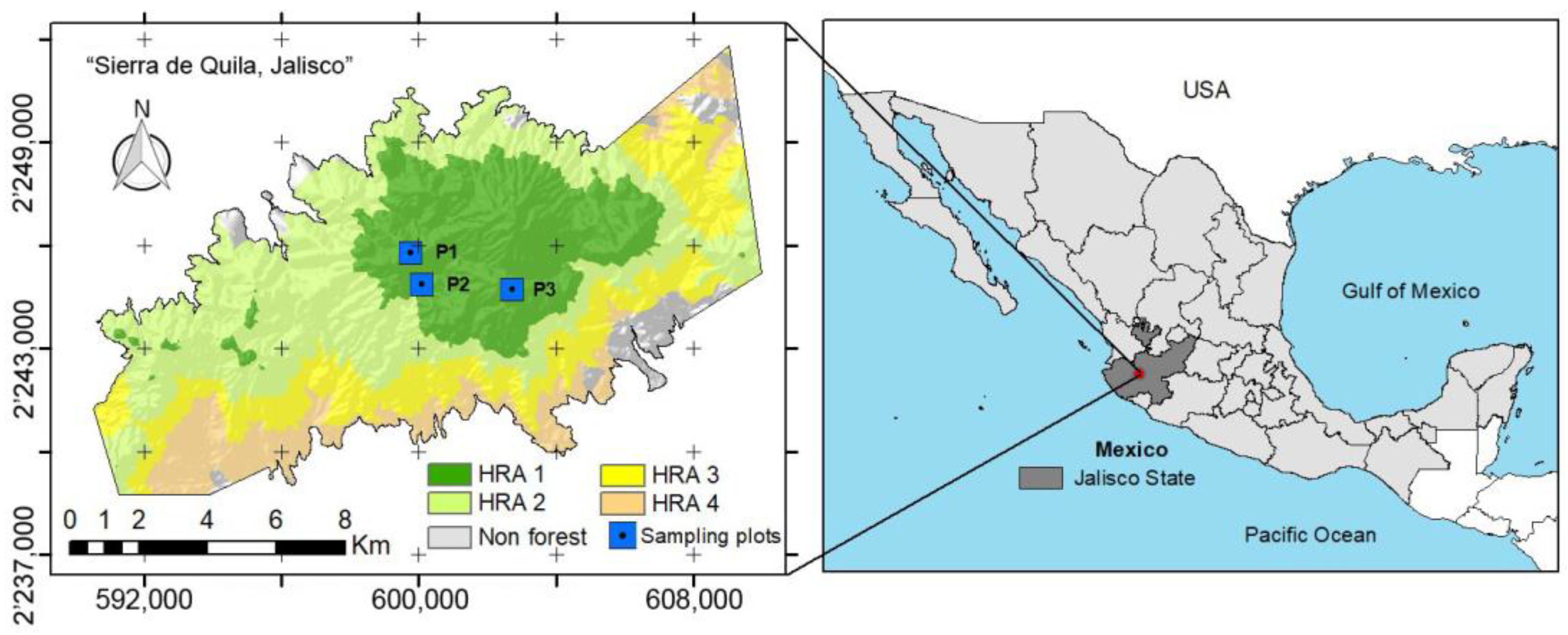
2.1. Study Area

This research was conducted in the natural protected area “Sierra de Quila”, located in west–central Mexico, in the state of Jalisco (Figure 1); the altitude ranges from 1350 to 2540 m asl. “Sierra de Quila” hosts many flora and fauna species that maintain important ecological processes enclosed in 15,192.50 ha [28]. Vegetation is mainly composed of mixed temperate forest with the following species: Pinus douglasiana, Pinus devoniana, Quercus resinosa, and Quercus obtusata. Potential fire regime is characterized by frequent surface fires of low severity [29]. However, a devastating crown fire occurred in 1986, resulting in both forest fighter and ecosystem property losses [30]. The study area is also prone to natural and human disturbances, such as insect outbreaks, firewood production, and timber harvesting. Previous studies have classified the area according to Homogeneous Response Areas (HRAs), where field information collected in situ can be extrapolated to areas with similar characteristics [31].

2.2. Materials, Data and Methods

The estimation of the spatial distribution of CFLs involved three key stages: data collection, data processing, and CFL mapping. The data collection phase encompassed both direct tree measurements in permanent sampling plots and data from UAV remote sensors. The processing phase involved estimation of both CFLs from field data and UAV imagery processing including digital photogrammetry methods, multispectral analysis, and three-dimensional data segmentation. Finally, the mapping phase comprised the application of Machine Learning techniques, specifically Random Forests, to estimate CFLs from remotely sensed data (Figure 2).

2.2.1. Field Data

Three square sampling permanent plots 1 ha (100 × 100 m) each were established in the study area. The plot’s corners were marked with 2 cm accuracy, using a Ruide Total Station RTS-833 georeferenced with a Topcon GR-5 Global Navigation Satellite System (GNSS). Reference coordinate system was the Universal Transverse Mercator Zone 13 North (UTM 13N) (Figure 1).
In each plot, all living trees with normal diameter (ND) greater than 5 cm [32] were measured and tagged in May 2022 (Figure 3. Field measurements and tree canopies overview). For each individual tree, its genus and species was recorded; the relative spatial location of each tree within the plot was mapped using a Suunto Tandem compass® (Suunto Oy, Vantaa, Finland) and a Truper® tape measure (Truper, Mexico City, Mexico). ND at 1.30 m above the ground was measured using a diameter tape Forestry Suppliers® (Forestry Suppliers Inc., Jackson, MS, USA). Crown diameter was determined with a Truper® tape measure (Truper, Mexico City, Mexico); total height was measured with a Suunto clinometer® (Suunto Oy, Vantaa, Finland).
CFLs for each tree were estimated using the allometric equations proposed by Rojas-García et al. (2015) [33], as described in Table 1. In addition, the following structural variables were estimated by tree genus by plot: mean height, sum of basal area, sum of ground crown cover, and mean square diameter [34]. Previous studies have shown that differences in tree spatial distribution patterns impact the accuracy of modeling the spatial distribution of above-ground biomass [35]. Therefore, in order to assess the effect of spatial patterns on CFL estimation, Moran’s Index was used; this index ranges from 1 (strong clustering) to −1 (strong dispersion), with 0 indicating a random pattern with no spatial autocorrelation. Tree location and CFLs were used to determine spatial patterns, according to Equation (1) [36].
I = n W i = 1 n j = 1 n W i , j z i z j i = 1 n z i 2
where I is Moran’s Index; n is number of observations; W is the sum of weights W i , j , z i is the difference of attribute in position i with respect to its mean ( X i X ¯ ), and z j is the difference of attribute in position j with respect to its mean ( X j X ¯ ).

2.2.2. Remote Sensing Data

UAV data were collected using a Sensefly Ebee® drone (AgEagle Aerial Systems Inc., Wichita, KS, USA), equipped with a Parrot Sequoia+® multispectral camera (Parrot, Paris, France) in September 2022. The sensor records spectral information in four bands: green (530–570 nm), red (640–680 nm), red edge (730–740 nm), and near-infrared (770–810 nm). Flight height was set to 212 m above the ground, resulting in a spatial resolution of 20 cm. Twenty-five images were captured per plot with 80% forward overlap and 60% side overlap. Prior to each flight, a target calibration panel was used to radiometrically correct the images [37]. Each multispectral flight was followed by a collection of RGB images, using a senseFly S.O.D.A 3D® camera (AgEagle Aerial Systems Inc., Wichita, KS, USA) (Figure 3D–F), using the same flight height above the ground, which resulted in a spatial resolution of 7 cm. Forward and side overlap was 60% and 70%, respectively, with twenty-two images captured per plot. For all flights, a set of ground control points (GCPs) were established along with flight plans through eMotion 3.5.0® software using grid flight missions for all flights [38]. The temporal lag between field and remote sensing data collection was based on tree species phenology [39,40].

2.2.3. Photogrammetric Point Clouds Generation

A Structure-from-Motion (SfM) algorithm was implemented to obtain three-dimensional data from S.O.D.A 3D® camera (AgEagle Aerial Systems Inc., Wichita, KS, USA), which enabled the reconstruction of the three-dimensional structure of a scene from a set of two-dimensional images [41]. This algorithm was executed using the Agisoft Metashape 1.6.4® software, which comprises three stages: (1) pre-processing, (2) densification, and (3) output generation.
The internal and relative orientation of individual images was applied based on their metadata spatial reference. Densification involved the assignment of descriptors to key points, which were matched using nearest-neighbor approximations and random sample consensus algorithms. Triangulation methods were used to estimate three-dimensional point positions and scene geometry reconstruction [41]. Point cloud, the three-dimensional collection of points in space representing the structure of the scene, was refined through the clustering stereoscopic multi-views algorithms [42]. Subsequently, relative coordinates were transformed into absolute coordinates by GCPs, achieving horizontal and vertical average RMSE values less than 0.50 m and 0.80 m, respectively. Point clouds were processed by linear triangulation resampling [43] and results were exported as point clouds and orthomosaic at the original spatial resolution.

2.2.4. Point Clouds Segmentation

Once the photogrammetric point clouds were generated, we attempted the identification of trees using a watershed-based approach. A point height normalization was first applied using the CloudCompare 2.12.4® software. The Cloth Simulation Filter (CSF) tool was used to filter point clouds into ground and non-ground data [44]. Ground returns were subsequently used to create a digital elevation model (DEM) and non-ground returns were used to generate digital surface models (DSM). The restricted ability of passive sensors to penetrate the canopy led to a scarcity of ground points, impeding the generation of a precise DEM. Therefore, it was necessary to use the National Institute of Statistic and Geography of Mexico (INEGI) DEM, with 15 m spatial resolution [45], to carry out point height normalization. The average ground slope was relatively constant, with values below 10% in each plot; with these values, it was feasible to use the DEM from INEGI, applying the nearest-neighbor resampling method [46] and using 1 m spatial resolution.
Subsequently, a Canopy Height Model (CHM) was generated, portraying the height of the crown trees in relation to the ground at a spatial resolution of 1 m. CHM segmentation (automatic delineation of trees in the scene) was performed using TREETOP, a Shiny-based application which was originally developed for the extraction of ecological information from airborne LiDAR data [47]. TREETOP detects individual trees and delineates crowns from CHM using the local maximum algorithm; this algorithm assumes that CHM local maxima represent the highest point of each tree [48]. Crown edges were segmented using the Voronoi Tessellation-based algorithm [49]. The segmented outputs did not align with individual trees, but they represented clusters of intermingled trees. After segmenting the tree crowns, the Canopy Volume of each segment (CV) was calculated based on the area and the height, derived from the CHM of the polygons [25], using the Python programming language [50].

2.2.5. Multispectral Analysis

Twelve vegetation indices (Table 2), together with homogeneity texture for each spectral band, were estimated; the moving window size considered in the analyses was 5 × 5 pixels. Spectral indices were used to estimate canopy fuel properties, including canopy fuel load [16]. Vegetation indices and textures were generated by multispectral orthomosaics [51]. One of the most efficient and widely used texture methods is the Gray Level Co-occurrence Matrix (GLCM) [52], whose features are based on neighboring pixel pair occurrence. This method produced different indicators such as contrast, correlation, energy, entropy, or homogeneity, among others. Homogeneity texture is widely used for its great importance in vegetation data due to its high level of detail [53]. Vegetation indices provide spectral insights linked to vegetation photosynthetic activity, vigor, status, and cover [54], and all are considered as valuable predictors of ecosystem features. To reduce the number of variables and to avoid collinearity of vegetation indices and texture variables, a principal components analysis (PCA), along with its factorial matrix, was carried out [55].

2.2.6. CFL Spatial Distribution

Segments extracted using TREETOP were aligned with field-acquired CFL data to derive reference values for CFLs. Descriptive statistics were estimated for all variables (i.e., CV, vegetation index, and texture metrics) for each segment. Differences among plots were tested by the non-parametric Kruskal–Wallis test as homoscedasticity was not fulfilled [66,67]; according to the Levene test, there was no homogeneity of variances among plots (p-value < 0.05).
The spatial distribution of CFLs was estimated by the Random Forest (RF) algorithm [68] using Python programming language [50]. RF is one of the most efficient Machine Learning algorithms [69], which implements a regression technique through bagging and random subspace methods [70]. The CFL was considered the response variable and CV, vegetation index, and textures as the explanatory variables. Segment metrics of the three plots were pooled and split into training data (70% of the sample) and validation data (30% of the sample). To train the model, 400 decision trees, bootstrap resampling, and square error were used [71]. The importance of each explanatory variable was evaluated through the mean decrease in impurity index (MDI) [72]. The algorithm was calibrated and applied using the following libraries: numpy [73], pandas [74], matplotlib [75], scikit [76], and GDAL OSGeo [77] for spatial data management.
The performance of the model was evaluated through the determination coefficient (R2) and Root Mean Square Error (RMSE) using validation data [68]. The RF-trained model was also applied over the total number of segments by plot; the R2 coefficient and absolute and relative CFL Bias were used to validate the accuracy across plots. The absolute Bias was calculated to evaluate the behavior of the RF-trained model on each plot and the relative Bias was used to compare plots [78]. Both estimations were performed according to Equations (2) and (3).
B i a s a b s = i N C F i ^ i N C F i
B i a s r e l = i N C F i ^ i N C F i i N C F i · 100
where B i a s a b s and B i a s r e l correspond to absolute and relative Bias, respectively; C F i ^ is the estimated CFL for each segment and C F i is the CFLs estimated from the field data.
Statistical analyses were carried out using the following R libraries “readr, northest, car, FactoMineR, and ggplot2” [79,80,81,82,83] available in R-project 4.3.0 [84].

3. Results

3.1. Plots’ Forest Structure

Three genus and twelve species were recorded within the plots (Table 1). The largest number of trees was recorded in P1, with 541 individuals, followed by P3, with 332 and P2 with 236. Pinus, followed by Quercus, was the dominant genus in all plots; Pinus exhibited the largest Quadratic Mean Diameter, Basal Area, Total Height, and Surface Crown Covered (Table 3). Pinus douglasiana and Quercus resinosa were the most abundant species in both genus. The highest CFL value was recorded in P1, with 163.47 Mg, followed by P2 and P3, with 151.07 Mg and 101.31 Mg, respectively. Pinus contributed the greatest amount of CFL in all plots, reaching values greater than 74% in each plot.
Distinct spatial distribution patterns were observed among the three plots (Table 4). In P1, both Pinus and Quercus exhibited clustering, whereas in P2, only Pinus formed clusters, with Quercus individuals displaying random distribution. In contrast, all trees in P3 were randomly distributed.

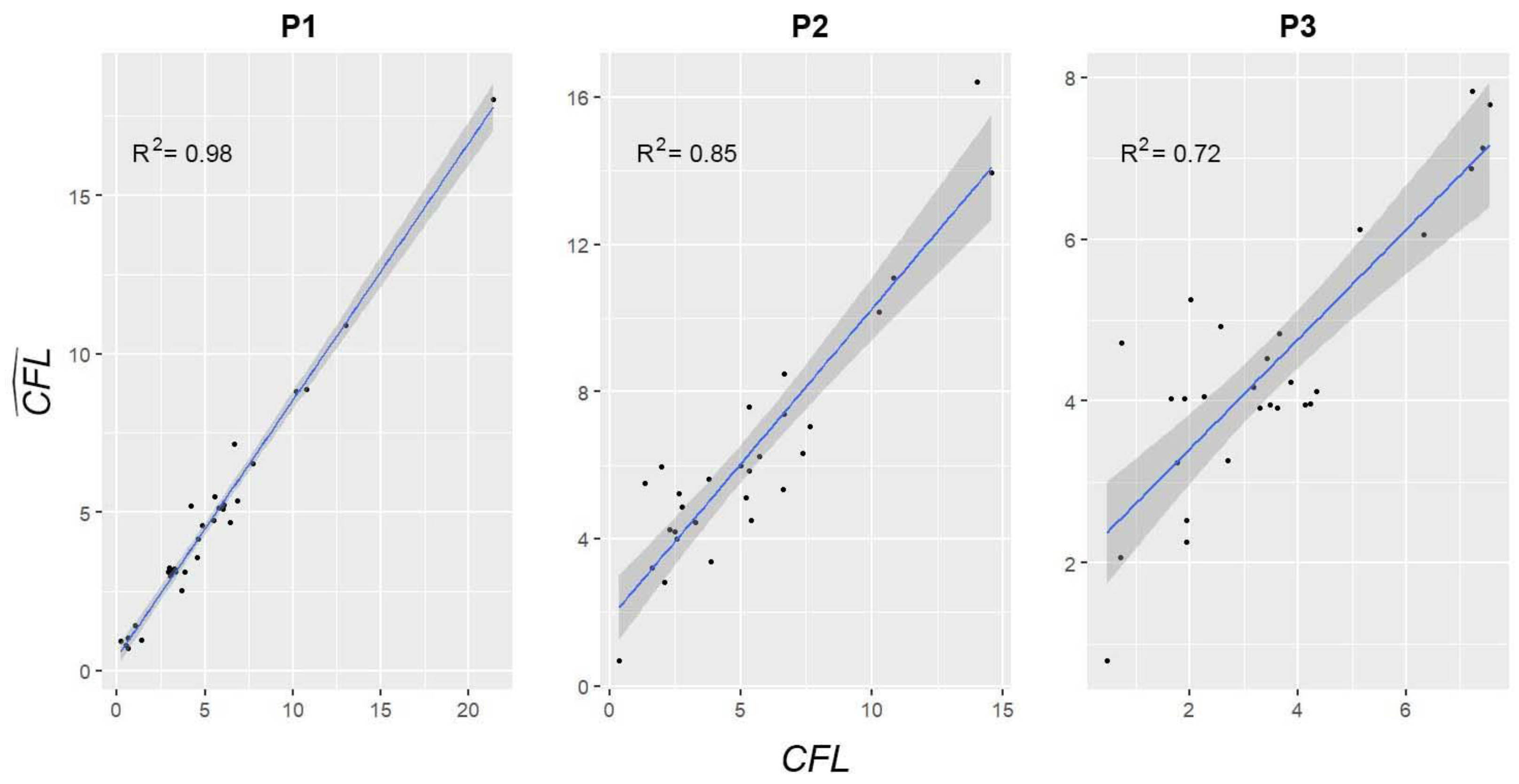
3.2. Remote Sensing Estimates

A set of multispectral orthomosaics and CHMs were obtained as a product of digital photogrammetry and point clouds processing. The mean CHM values were 17.84 m, 21.95 m, and 20.73 m in P1, P2, and P3, respectively. The segmentation analysis identified 31, 28, and 28 segments, covering 7883 m2, 8104 m2, and 8782 m2 in P1, P2, and P3, respectively (Figure 4).
The number of trees identified using TREETOP was 511, 229, and 322 for P1, P2, and P3, respectively. These values represented a detection rate of 94.5%, 97%, and 97.3% for P1, P2, and P3. The absence of certain trees within each plot led to a minor underestimation of CFLs at the plot level when focusing solely on the fuel load of the trees correctly detected (161.02 Mg, 147.60 Mg, and 98.61 Mg in P1, P2, and P3, respectively), as indicated in Table 3. P1 had the lowest omission in terms of CFL, despite the lowest detection rate, with 1.50%, followed by P2 with 2.29% and P3 with 2.67%.
According to the factorial matrix from the PCA, four variables were uncorrelated, exhibiting a robust relationship with the first three principal components: Normalized Difference Vegetation Index (NDVI), 2-band Enhanced Vegetation Index (EVI2), Red band homogeneity texture and Red edge band homogeneity texture.
The median CFL values per segment were 4.54 Mg, 5.09 Mg, and 3.35 Mg in P1, P2, and P3, respectively (Figure 5A), with no significant differences according to the Kruskal–Wallis test: H(2) = 3.64, p = 0.16. There were statistically significant differences for CV, vegetation index, and textures among plots. For CV, H(2) = 11.96, p < 0.05, with median values of 4000.66, 6740.58, and 6590.29 m3 for P1, P2, and P3, respectively (Figure 5B). Finally, for the NDVI, EVI2, Red band texture and Red edge band texture, the results were H(2) = 56.73 with p < 0.05, H(2) = 33.00, p < 0.05, H(2) = 36.96, p < 0.05, and H(2) = 12.48, p < 0.05, respectively (Figure 5C–F).

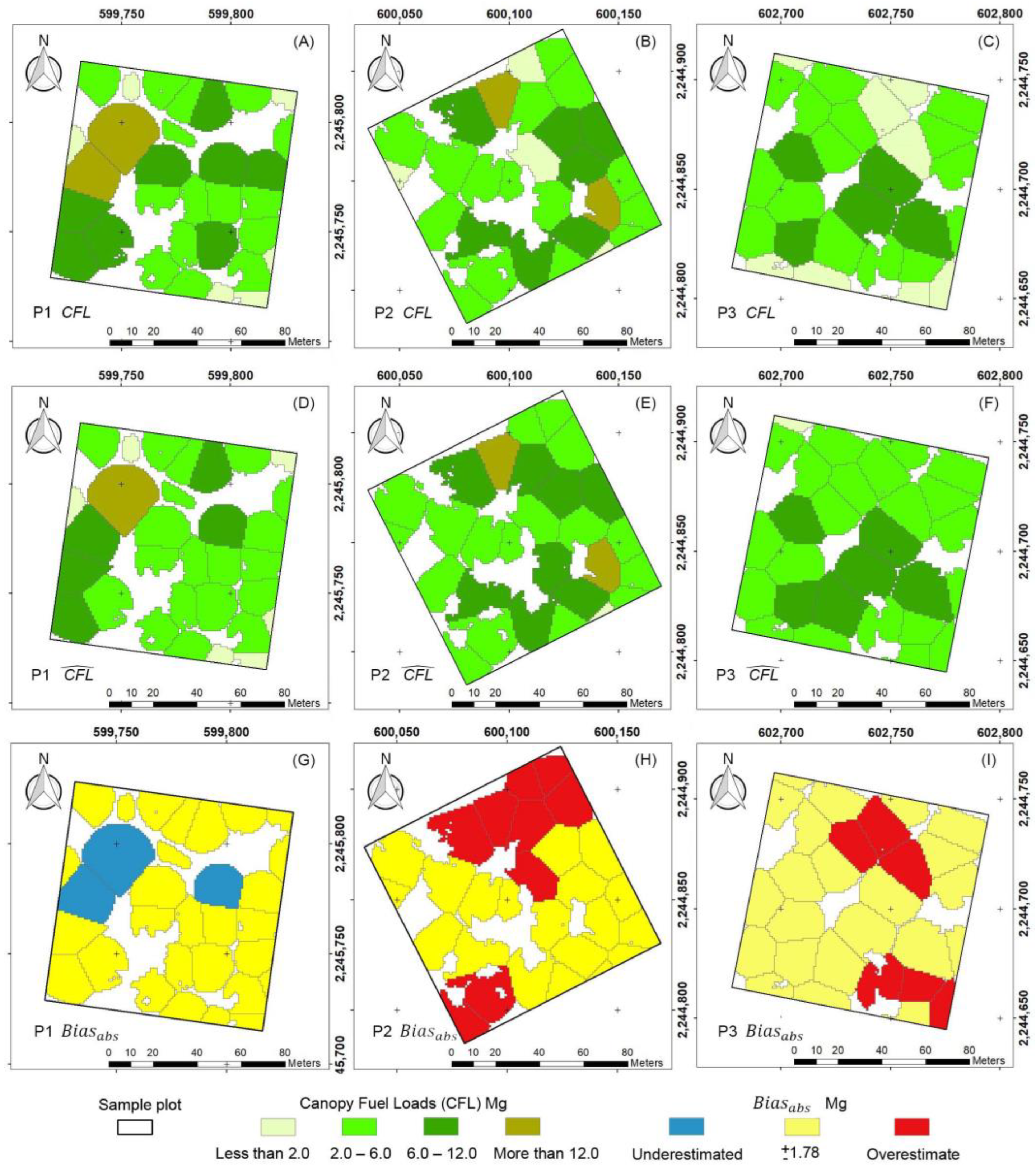
3.3. Spatial Distribution of CFLs

According to validation data, our RF model achieved a strong performance with R2 = 0.75 and RMSE = 1.78 Mg. At the plot level, P1 reached R2 = 0.98, B i a s a b s = −17.12 Mg, and B i a s r e l = 10.63%; P2 yielded R2 = 0.85, B i a s a b s = 28.06 Mg, and B i a s r e l = 19.01%; and P3 offered a performance of R2 = 0.72, B i a s a b s = 25.85 Mg, and B i a s r e l = 26.21%. (Figure 6). Therefore, the modeled CFL per plot was 143.90 Mg, 175.66 Mg, and 124.46 Mg for P1, P2, and P3, respectively (Figure 7D–F).
The most significant variable was CV, at 80.67%, followed by Red band texture at 7.00%, Red edge band texture at 5.99%, NDVI at 4.15%, and EVI2 ay 2.19%.

4. Discussion

The spatial distribution of the CFL, estimated through a combination of digital photogrammetry, segmentation, multispectral analysis, and Machine Learning, yielded robust results, according to R2, RMSE, and Bias. The study of CFLs in mixed forests with structural complexity and different spatial distribution patterns was conducted through the integration of various techniques. These techniques allowed for a more comprehensive analysis and understanding of the CFL in the complex nature of mixed forests of the “Sierra de Quila”.

4.1. Plots Forest Structure

The Pinus genus exhibited the highest CFL values, contributing to over 70% in each plot. This aligns with the findings of a previous study by Villavicencio-García et al. (2005) [85], which investigated the entire altitudinal gradient of “Sierra de Quila” and identified species from the Pinus genus as dominant. Typically, Pinus species occupy the upper canopy, while Quercus species tend to dominate the middle canopy, with tree crowns in close proximity or even overlapping [86]. In many regions, including areas like “Sierra de Quila”, most Pinus species in Mexico rely on fire, with these regions characterized by frequent surface fires of low severity [29,87].
In the present study, the Pinus genus presented the highest values in structural variables such as quadratic mean diameter, basal area, tree height, and vegetation cover. This result is highly relevant as values of the CFL depend on tree structural variables [33]. Previous studies by Figueroa-Navarro et al. (2023) in “Sierra de Quila” [88] obtained similar results to those achieved in the present work, with average densities of 556 trees per ha and a mean basal area of 20 m2/ha, with Pinus douglasiana being the most dominant species, regarding Pinus genus and Quercus resinosa as the most dominant species of the Quercus genus.
Tree spatial distribution patterns differed among the three plots according to Moran´s Index. Moreover, differences among the plots also occurred in terms of CFLs. Thus, the highest degree of clustering was present in P1, showing the greatest values of CFLs (median value of 16.98 kg/m2). Conversely, the greatest random pattern was observed in P3, presenting the lowest CFL values (median value of 10.71 kg/m2). These differences limit the use of linear and allometric model regression because tree spatial distribution patterns prevent generalizable models from being obtained [89,90]. Other studies have identified that mixed forests tend to present random distributions following a disturbance occurrence and they are reverted to clusters over time [91]; therefore, these may be the cause of differences in the spatial distribution patterns of trees in our study area.

4.2. Remote Sensing

Information derived from the photogrammetric point clouds provided valuable results by capturing significant three-dimensional information on trees, despite the fact that LiDAR data lack penetration ability [92]. Mixed forests in Mexico make it difficult to accurately estimate CFLs, mainly due to the high tree density that results in crowns close to each other or even overlapping. In such forest types, estimates focusing on crown segments, rather than on individual trees, provide a viable alternative [93]. CV has been a good alternative for estimates focusing on crown segments. This agrees with Riggi et al. (2021) [25], who used CV to estimate the above-ground biomass of olive plantations by linear regression models, reaching up to R2 = 0.68 and RMSE = 39.19 kg. In our work, mixed forests presented greater structural complexity, with irregular spatial distribution of trees. Nevertheless, texture and vegetation indices included in the RF algorithm proved to be a valuable complement to CV, allowing the inclusion of differences in trees’ spatial distribution patterns between plots [51].
Despite the more limited information extracted from photogrammetric point clouds as compared to LiDAR point clouds, our results showed strong agreement with field estimates of CFLs. Thus, CFL differences within the segments were less than 3% compared to the total CFLs measured in the field. This remarkable agreement could be attributed to the size of the plots used, which were notably larger than those used in other studies. This factor contributed to minimizing the border effect. Tree trunks typically deviate for a vertical orientation, resulting in a discrepancy between their geolocation and the boundaries of segments. This border effect is mostly evident in small plots, while in large plots this error tends to be compensated [15]. According to Knapp et al. (2018) [94], to attain precisions with errors below <10%, sample plots must be of at least 100 m per side. Our plots measured 100 m on each side, enabling the segmentation process and field measurements to capture the inherent three-dimensional spatial distribution of the trees in accordance with their spatial variability.

4.3. Spatial Distribution of CFLs

The RF regression model enabled an accurate description of the spatial distribution of CFLs within our plots. The trained model achieved errors of less than 30%, even when trees had different patterns of spatial distribution. The lowest errors were observed in P1, where trees showed the highest density. These contrast with the findings of Guerra-Hernández et al. (2016) [95], who suggested that higher-density plots may yield inaccurate results due to the limited penetration of photogrammetric point clouds into the canopy. In our case, we addressed this situation by incorporating multispectral data and textures, along with the segmentation approach based on surfaces rather than on individual trees. In addition, employing an external DEM with proven accuracy contributed to enhancing our estimates of the structure metrics derived from UAV data. The results in this study were similar to those reported by Maesano et al. (2022) [24], who achieved B i a s r e l close to 10% by combining data from LiDAR, RGB images, and RF algorithms. This confirms that our approach enables the development of robust and accurate models, even in the absence of LiDAR data.
According to the MDI, CV was the most important variable of the model, accounting for over 80%. In contrast, the texture and vegetation indices, considered together, showed importance values close to 20%. The influence of CV on accuracy was substantial, particularly in instances where trees exhibited clustered spatial distribution patterns, leading to improved model performance. Moreover, texture and spectral indices were useful in overcoming the limitations of point clouds and addressing the structural complexity inherent in mixed forests [51,54].
The developed method offers high potential to accurately estimate CFLs within the context of native mixed forests characterized by a complex spatial distribution of trees, even in the absence of LiDAR data. The proposed method for mapping CFLs’ spatial distribution not only allows for the optimization of costs and time associated with intensive field measurements [10] but also serves as a cost-effective alternative to LiDAR technology [96]. In this research, sampling plots showed relatively low ground and slope values, staying below 10%. The accuracy may be impacted in areas with higher slopes or predominantly rugged terrain; therefore, a DEM should be applied instead of a DSM. However, this situation can be solved using topographic measurements.
The field data utilized in this research belong to the same HRA of the study area, where they share a common ecological background. This context enables in situ data collection to extrapolate to areas with similar characteristics [31]. However, the robustness of the method ensures its replicability across various latitudes. Moreover, it is feasible to extend its applicability from a local geographic scope to wider areas thought upscaling techniques [17,22]. The present method uses data from field measurements, digital photogrammetry, multispectral analysis, and Machine Learning techniques, mostly through open source software; the method is also straightforward to implement. Although the method has undergone local testing, its transferability to other areas is seamless, facilitated by the easy and cost-effective collection of data across diverse geographical regions.
After collecting field measurements, the proposed method requires only a few hours for data processing. Moreover, trained Machine Learning models can be used in areas with similar ecological context, allowing forest managers to make informed decisions based on current and reliable information.

5. Conclusions

The present research introduces a methodology for mapping the spatial distribution of CFLs by employing image segmentation, multispectral analysis, and Machine Learning modeling. This approach enables the extraction of structural information, yielding commendable accuracy in CFL estimation. Mapping CFLs was consistent even when the study area presented a high level of complexity pertaining to the mixture of genera and species in the forest and the variation in patterns of the trees’ spatial distribution. Machine Learning modeling, in particular RF based on CV complemented with multispectral variables derived at the object level, enabled a high accuracy at a relatively low cost.
This method can be easily applied to drone-derived data, which is particularly important in areas with frequent disturbances, to obtain reliable and updated information for decision making. The present method offers the opportunity for CFL monitoring, which can be used to generate models of temporal dynamics and their interactions with the environment.
The investigation of the complex of forest fuels holds a pivotal position in fire research, accenting the overriding significance of studying the spatial distribution of CFLs. This exploration is essential for depicting the intricate nature of the fuel complex, comprehending its dynamics, and unraveling spatial variability within the broader ecological framework. Such insights are indispensable for researchers, academics, and forest managers alike, providing a central foundation for making informed decisions regarding the management of forest fuels and the mitigation of forest fires.

Author Contributions

Conceptualization, M.G., I.A., M.O.-V., B.L.F.-R. and Á.A.C.-D.; data curation, M.G. and Á.A.C.-D.; formal analysis, M.G., I.A., M.O.-V., B.L.F.-R., R.T.-C., E.A.R.-C. and Á.A.C.-D.; funding acquisition, M.G. and M.O.-V.; methodology, M.G., I.A., M.O.-V., B.L.F.-R. and Á.A.C.-D.; software, M.G., R.T.-C. and Á.A.C.-D.; validation, M.G., I.A., M.O.-V., B.L.F.-R. and Á.A.C.-D.; visualization, M.G., I.A. and Á.A.C.-D.; writing—original draft, Á.A.C.-D.; writing—review and editing, M.G., I.A., M.O.-V., B.L.F.-R., R.T.-C., E.A.R.-C. and Á.A.C.-D. All authors have read and agreed to the published version of the manuscript.

Funding

This research was funded by a National Committee of Humanities, Science and Technology (CONAHCyT) of Mexico Unique Curriculum Vitae Scholarship (CVU): 167647 and a Grant for Excellence in Teaching Staff of the Community of Madrid (EPU-DPTO/2020/008).

Data Availability Statement

Dataset available on request from the authors.

Acknowledgments

We would like to thank the anonymous reviewers for their constructive suggestions, which helped to improve our paper. To the department for their support: Grant for Excellence in Teaching Staff of the Community of Madrid (EPU-DPTO/2020/008); to the National Committee of Humanities, Science and Technology (CONAHCyT) of Mexico for their support in carrying out this work; to the Natural Protected Area of “Sierra de Quila”, Jalisco, Mexico for their active participation and operational support in carrying out this work; to the National Institute of Forestry, Agricultural and Livestock Research of Mexico (INIFAP) for the facilities granted in the research tasks; and to Enrique Miguel Valle, Abundio Bustos Santana, Rafael Sevilla Pérez, Gustavo Eduardo Flores Tomás, Candelario Calderón Santana, Alfredo Sedano Gutiérrez, Roberto Ponce Sánchez, Roberto Zepeda Camberos, Alvaro Pujol Becerra, Ulises Vladimir Chávez Durán, José Gildardo López Beltrán, Emmanuel López Solórzano, and Manuel Durán Rolón for their technical and operational support in the fieldwork.

Conflicts of Interest

The authors declare no conflicts of interest.

References

  1. Pyne, S.J.; Andrews, P.L.; Laven, R.D. Introduction to Wildland Fire, 2nd ed.; Wiley: New York, NY, USA, 1996. [Google Scholar]
  2. Keane, R.E. Wildland Fuel Fundamentals and Applications; Springer International: New York, NY, USA, 2015. [Google Scholar]
  3. United States Department of Agriculture, Forest Service (USDA). Fuels Management. Available online: https://www.fs.usda.gov/ (accessed on 16 September 2023).
  4. Weise, D.R.; Cobian-Iñiguez, J.; Princevac, M. Surface to Crown Transition. In Encyclopedia of Wildfires and Wildland-Urban Interface (WUI) Fires; Springer International Publishing: Cham, Switzerland, 2018; pp. 1–5. [Google Scholar] [CrossRef]
  5. Scott, J.H.; Reinhardt, E.D. Assessing Crown Fire Potential by Linking Models of Surface and Crown Fire Behavior; U.S. Department of Agriculture, Forest Service, Rocky Mountain Research Station: Fort Collins, CO, USA, 2001. [CrossRef]
  6. Maesano, M.; Ottaviano, M.; Lidestav, G.; Lasserre, B.; Matteucci, G.; Scarascia Mugnozza, G.; Marchetti, M. Forest Certification Map of Europe. IForest 2018, 11, 526–533. [Google Scholar] [CrossRef]
  7. Dang, A.T.N.; Nandy, S.; Srinet, R.; Luong, N.V.; Ghosh, S.; Senthil Kumar, A. Forest Aboveground Biomass Estimation Using Machine Learning Regression Algorithm in Yok Don National Park, Vietnam. Ecol. Inf. 2019, 50, 24–32. [Google Scholar] [CrossRef]
  8. Skowronski, N.S.; Clark, K.L.; Duveneck, M.; Hom, J. Three-Dimensional Canopy Fuel Loading Predicted Using Upward and Downward Sensing LiDAR Systems. Remote Sens. Environ. 2011, 115, 703–714. [Google Scholar] [CrossRef]
  9. Mallinis, G.; Mitsopoulos, Ι.; Stournara, P.; Patias, P.; Dimitrakopoulos, A. Canopy Fuel Load Mapping of Mediterranean Pine Sites Based on Individual Tree-Crown Delineation. Remote Sens. 2013, 5, 6461–6480. [Google Scholar] [CrossRef]
  10. Stereńczak, K.; Mielcarek, M.; Wertz, B.; Bronisz, K.; Zajączkowski, G.; Jagodziński, A.M.; Ochał, W.; Skorupski, M. Factors Influencing the Accuracy of Ground-Based Tree-Height Measurements for Major European Tree Species. J. Environ. Manag. 2019, 231, 1284–1292. [Google Scholar] [CrossRef]
  11. Tadese, S.; Soromessa, T.; Bekele, T.; Bereta, A.; Hailemariam, F. Above Ground Biomass Estimation Methods and Challenges: A Review. J. Energy Technol. Policy 2019, 9, 1–14. [Google Scholar] [CrossRef]
  12. Prichard, S.J.; Andreu, A.G.; Ottmar, R.D.; Eberhardt, E. Fuel Characteristic Classification System (FCCS) Field Sampling and Fuelbed Development Guide; United States Department of Agriculture: Portland, OR, USA, 2019. [CrossRef]
  13. Chávez-Durán, Á.A.; Flores-Garnica, J.G.; Luna-Luna, M.; Centeno-Erguera, L.R.; Alarcón-Bustamante, M.P. Caracterización y Clasificación de Camas de Combustibles Prioritarias En México Para Planificar El Manejo Del Fuego. Informe Técnico Fondo Sectorial CONACyT-CONAFOR. Referencia: CONAFOR-2012-C01-175523; Sistema Nacional de Información y Gestión Forestal: Tepatitlán de Morelos, Mexico, 2014. Available online: http://www.cnf.gob.mx/IMASD (accessed on 16 August 2022).
  14. Ortíz-Mendoza, R.; Martínez-Torres, H.L.; Pérez-Salicrup, D.R.; Garduño-Mendoza, E.; Oceguera-Salazar, K.A. Caracterización y Clasificación de Combustibles Para Generar y Validar Modelos de Combustibles Forestales Para México. CONAFOR-CONACyT 2014-251694. Metodología y Guía de Campo Para La Medición de Cargas de Camas de Combustibles Forestales y Ambientes Del Fuego; CONAFOR: Morelia, Mexico, 2017. Available online: http://www.cnf.gob.mx/IMASD (accessed on 16 September 2023).
  15. Zolkos, S.G.; Goetz, S.J.; Dubayah, R. A Meta-Analysis of Terrestrial Aboveground Biomass Estimation Using Lidar Remote Sensing. Remote Sens. Environ. 2013, 128, 289–298. [Google Scholar] [CrossRef]
  16. Barrett, F.; McRoberts, R.E.; Tomppo, E.; Cienciala, E.; Waser, L.T. A Questionnaire-Based Review of the Operational Use of Remotely Sensed Data by National Forest Inventories. Remote Sens. Environ. 2016, 174, 279–289. [Google Scholar] [CrossRef]
  17. García, M.; Saatchi, S.; Casas, A.; Koltunov, A.; Ustin, S.; Ramirez, C.; Balzter, H. Extrapolating Forest Canopy Fuel Properties in the California Rim Fire by Combining Airborne LiDAR and Landsat OLI Data. Remote Sens. 2017, 9, 394. [Google Scholar] [CrossRef]
  18. García, M.; Danson, F.M.; Riaño, D.; Chuvieco, E.; Ramirez, F.A.; Bandugula, V. Terrestrial Laser Scanning to Estimate Plot-Level Forest Canopy Fuel Properties. Int. J. Appl. Earth Obs. Geoinf. 2011, 13, 636–645. [Google Scholar] [CrossRef]
  19. García, M.; Popescu, S.; Riaño, D.; Zhao, K.; Neuenschwander, A.; Agca, M.; Chuvieco, E. Characterization of Canopy Fuels Using ICESat/GLAS Data. Remote Sens. Environ. 2012, 123, 81–89. [Google Scholar] [CrossRef]
  20. Jiang, F.; Deng, M.; Tang, J.; Fu, L.; Sun, H. Integrating Spaceborne LiDAR and Sentinel-2 Images to Estimate Forest Aboveground Biomass in Northern China. Carbon. Balance Manag. 2022, 17, 12. [Google Scholar] [CrossRef]
  21. Moran, C.J.; Kane, V.R.; Seielstad, C.A. Mapping Forest Canopy Fuels in the Western United States with LiDAR–Landsat Covariance. Remote Sens. 2020, 12, 1000. [Google Scholar] [CrossRef]
  22. Bergamo, T.F.; de Lima, R.S.; Kull, T.; Ward, R.D.; Sepp, K.; Villoslada, M. From UAV to PlanetScope: Upscaling Fractional Cover of an Invasive Species Rosa Rugosa. J. Environ. Manag. 2023, 336, 117693. [Google Scholar] [CrossRef]
  23. Mao, P.; Ding, J.; Jiang, B.; Qin, L.; Qiu, G.Y. How Can UAV Bridge the Gap between Ground and Satellite Observations for Quantifying the Biomass of Desert Shrub Community? ISPRS J. Photogramm. Remote Sens. 2022, 192, 361–376. [Google Scholar] [CrossRef]
  24. Maesano, M.; Santopuoli, G.; Moresi, F.; Matteucci, G.; Lasserre, B.; Scarascia Mugnozza, G. Above Ground Biomass Estimation from UAV High Resolution RGB Images and LiDAR Data in a Pine Forest in Southern Italy. IForest 2022, 15, 451–457. [Google Scholar] [CrossRef]
  25. Riggi, E.; Avola, G.; Di Gennaro, S.F.; Cantini, C.; Muratore, F.; Tornambè, C.; Matese, A. UAV-Based 3D Models of Olive Tree Crown Volumes for above-Ground Biomass Estimation. Acta Hortic. 2021, 1314, 353–360. [Google Scholar] [CrossRef]
  26. Zhang, Z.; Zhu, L. A Review on Unmanned Aerial Vehicle Remote Sensing: Platforms, Sensors, Data Processing Methods, and Applications. Drones 2023, 7, 398. [Google Scholar] [CrossRef]
  27. Duff, T.; Keane, R.; Penman, T.; Tolhurst, K. Revisiting Wildland Fire Fuel Quantification Methods: The Challenge of Understanding a Dynamic, Biotic Entity. Forests 2017, 8, 351. [Google Scholar] [CrossRef]
  28. Comisión Nacional de Áreas Naturales Protegidas (CONANP). Recategorización Del Área de Protección de Flora y Fauna “Sierra de Quila”; Diario Oficial: Mexico City, Mexico, 2000; pp. 1–5. Available online: https://simec.conanp.gob.mx/pdf_recategorizacion/64_reca.pdf (accessed on 27 June 2022).
  29. Jardel-Pelaez, E.J.; Pérez-Salicrup, D.; Alvarado-Celestino, E.; Morfin-Rios, J.E. Principios y Criterios Para El Manejo Del Fuego En Ecosistemas Forestales: Guía de Campo; Comisión Nacional Forestal: Guadalajara, Mexico, 2014.
  30. Jiménez-Luquín, E. Sierra de Quila: Cómo Ha Ido Cambiando Los Últimos 25 Años Desde La Tragedia? In Memorias. I Foro de Conocimiento, uso y Gestión del Área Natural Protegida Sierra de Quila; Villavicencio-García, R., Santiago-Pérez, A.L., Rosas-Espinoza, V.C., Hernández-López, L., Eds.; Universidad de Guadalajara, Centro Universitario de Ciencias Biológicas y Agropecuarias, Departamento de Producción Forestal: Guadalajara, Mexico, 2011; pp. 1–134. [Google Scholar]
  31. Chávez-Durán, Á.A.; Olvera-Vargas, M.; Figueroa-Rangel, B.; García, M.; Aguado, I.; Ruiz-Corral, J.A. Mapping Homogeneous Response Areas for Forest Fuel Management Using Geospatial Data, K-Means, and Random Forest Classification. Forests 2022, 13, 1970. [Google Scholar] [CrossRef]
  32. Olvera-Vargas, M.; Moreno-Gómez, S.; Figueroa-Rangel, B. Sitios Permanentes Para La Investigación Silvícola. Manual Para Su Establecimiento, 1st ed.; Universidad de Guadalajara: Guadalajara, Mexico, 1996; Volume 1. [Google Scholar]
  33. Rojas-García, F.; De Jong, B.H.J.; Martínez-Zurimendí, P.; Paz-Pellat, F. Database of 478 Allometric Equations to Estimate Biomass for Mexican Trees and Forests. Ann. Sci. 2015, 72, 835–864. [Google Scholar] [CrossRef]
  34. Bettinger, P.; Boston, K.; Siry, J.; Grebner, D. Forest Management and Planning, 2nd ed.; Academic Press: San Diego, CA, USA, 2016. [Google Scholar]
  35. Pizaña, J.M.G.; Hernández, J.M.N.; Romero, N.C. Remote Sensing-Based Biomass Estimation. In Environmental Applications of Remote Sensing; Marghany, M., Ed.; InTech: London, UK, 2016. [Google Scholar] [CrossRef]
  36. Siabato, W.; Guzmán-Manrique, J. La Autocorrelación Espacial y El Desarrollo de La Geografía Cuantitativa. Cuad. De Geogr. Rev. Colomb. De Geogr. 2019, 28, 1–22. [Google Scholar] [CrossRef]
  37. Poncet, A.M.; Knappenberger, T.; Brodbeck, C.; Fogle, M.; Shaw, J.N.; Ortiz, B.V. Multispectral UAS Data Accuracy for Different Radiometric Calibration Methods. Remote Sens. 2019, 11, 1917. [Google Scholar] [CrossRef]
  38. Park, J.W.; Yeom, D.J. Method for Establishing Ground Control Points to Realize UAV-Based Precision Digital Maps of Earthwork Sites. J. Asian Archit. Build. Eng. 2022, 21, 110–119. [Google Scholar] [CrossRef]
  39. Fideicomiso para la Administración del Programa de Desarrollo Forestal del Estado (FIPRODEFO). Monografías de Pinos Nativos Promisorios Para Plantaciones Forestales Comerciales En Jalisco, México; FIPRODEFO: Guadalajara, Mexico, 2001. Available online: https://geoportal.fiprodefo.gob.mx (accessed on 9 November 2023).
  40. Pérez-Mojica, E.; Valencia-A., S. Estudio Preliminar Del Género Quercus (Fagaceae) En Tamaulipas, México. Acta Bot. Mex. 2017, 120, 59–111. [Google Scholar] [CrossRef]
  41. Westoby, M.J.; Brasington, J.; Glasser, N.F.; Hambrey, M.J.; Reynolds, J.M. ‘Structure-from-Motion’ Photogrammetry: A Low-Cost, Effective Tool for Geoscience Applications. Geomorphology 2012, 179, 300–314. [Google Scholar] [CrossRef]
  42. Furukawa, Y.; Curless, B.; Seitz, S.M.; Szeliski, R. Towards Internet-Scale Multi-View Stereo. In Proceedings of the 2010 IEEE Computer Society Conference on Computer Vision and Pattern Recognitio, San Francisco, CA, USA, 13–18 June 2010; pp. 1434–1441. [Google Scholar] [CrossRef]
  43. Agisoft LLC. Agisoft Metashape User Manual; Agisoft LLC.: St. Petersburg, Russia, 2023. [Google Scholar]
  44. CloudCompare. 3D Point Cloud and Mesh Processing Software Open Source Project. Available online: https://www.danielgm.net/cc/ (accessed on 4 January 2023).
  45. Instituto Nacional de Estadística y Geografía (INEGI). Continuo de Elevaciones Mexicano 3.0; INEGI: Aguascalientes, Mexico, 2013. Available online: https://www.inegi.org.mx/app/geo2/elevacionesmex/ (accessed on 7 February 2023).
  46. Baboo, S.; Devi, R. An Analysis of Different Resampling Methods in Coimbatore, District. Glob. J. Comput. Sci. Technol. 2010, 10, 61–66. [Google Scholar]
  47. Silva, C.A.; Hudak, A.T.; Vierling, L.A.; Valbuena, R.; Cardil, A.; Mohan, M.; Almeida, D.R.A.; Broadbent, E.N.; Almeyda Zambrano, A.M.; Wilkinson, B.; et al. TREETOP: A Shiny-Based Application and R Package for Extracting Forest Information from LiDAR Data for Ecologists and Conservationists. Methods Ecol. Evol. 2022, 13, 1164–1176. [Google Scholar] [CrossRef]
  48. Korpela, I.; Anttila, P.; Pitkänen, J. The Performance of a Local Maxima Method for Detecting Individual Tree Tops in Aerial Photographs. Int. J. Remote Sens. 2006, 27, 1159–1175. [Google Scholar] [CrossRef]
  49. Silva, C.A.; Hudak, A.T.; Vierling, L.A.; Loudermilk, E.L.; O’Brien, J.J.; Hiers, J.K.; Jack, S.B.; Gonzalez-Benecke, C.; Lee, H.; Falkowski, M.J.; et al. Imputation of Individual Longleaf Pine (Pinus Palustris Mill.) Tree Attributes from Field and LiDAR Data. Can. J. Remote Sens. 2016, 42, 554–573. [Google Scholar] [CrossRef]
  50. Python. Python Software Foundation. Available online: https://www.python.org/ (accessed on 15 June 2023).
  51. Mohammadpour, P.; Viegas, D.X.; Viegas, C. Vegetation Mapping with Random Forest Using Sentinel 2 and GLCM Texture Feature—A Case Study for Lousã Region, Portugal. Remote Sens. 2022, 14, 4585. [Google Scholar] [CrossRef]
  52. Kupidura, P. The Comparison of Different Methods of Texture Analysis for Their Efficacy for Land Use Classification in Satellite Imagery. Remote Sens. 2019, 11, 1233. [Google Scholar] [CrossRef]
  53. Katoh, M.; Gougeon, F.A. Improving the Precision of Tree Counting by Combining Tree Detection with Crown Delineation and Classification on Homogeneity Guided Smoothed High Resolution (50 cm) Multispectral Airborne Digital Data. Remote Sens. 2012, 4, 1411–1424. [Google Scholar] [CrossRef]
  54. Guerini Filho, M.; Kuplich, T.M.; De Quadros, F.L.F. Estimating Natural Grassland Biomass by Vegetation Indices Using Sentinel 2 Remote Sensing Data. Int. J. Remote Sens. 2020, 41, 2861–2876. [Google Scholar] [CrossRef]
  55. Greenacre, M.; Groenen, P.J.F.; Hastie, T.; D’Enza, A.I.; Markos, A.; Tuzhilina, E. Principal Component Analysis. Nat. Rev. Methods Primers 2022, 2, 100. [Google Scholar] [CrossRef]
  56. Rouse, J.W.; Haas, R.H.; Schell, J.A.; Deering, D.W. Monitoring Vegetation Systems in the Great Plains with Erts. NASA Spec. Publ. 1974, 351, 309–317. [Google Scholar]
  57. Huete, A.R. A Soil-Adjusted Vegetation Index (SAVI). Remote Sens. Environ. 1988, 25, 295–309. [Google Scholar] [CrossRef]
  58. Qi, J.; Chehbouni, A.; Huete, A.R.; Kerr, Y.H.; Sorooshian, S. A Modified Soil Adjusted Vegetation Index. Remote Sens. Environ. 1994, 48, 119–126. [Google Scholar] [CrossRef]
  59. Jiang, Z.; Huete, A.; Didan, K.; Miura, T. Development of a Two-Band Enhanced Vegetation Index without a Blue Band. Remote Sens. Environ. 2008, 112, 3833–3845. [Google Scholar] [CrossRef]
  60. Richardson, A.J.; Everitt, J.H. Using Spectral Vegetation Indices to Estimate Rangeland Productivity. Geocarto Int. 1992, 7, 63–69. [Google Scholar] [CrossRef]
  61. Gitelson, A.A.; Kaufman, Y.J.; Merzlyak, M.N. Use of a Green Channel in Remote Sensing of Global Vegetation from EOS-MODIS. Remote Sens. Environ. 1996, 58, 289–298. [Google Scholar] [CrossRef]
  62. Sripada, R.P.; Heiniger, R.W.; White, J.G.; Meijer, A.D. Aerial Color Infrared Photography for Determining Early In-Season Nitrogen Requirements in Corn. Agron. J. 2006, 98, 968–977. [Google Scholar] [CrossRef]
  63. Gianelle, D.; Vescovo, L. Determination of Green Herbage Ratio in Grasslands Using Spectral Reflectance. Methods and Ground Measurements. Int. J. Remote Sens. 2007, 28, 931–942. [Google Scholar] [CrossRef]
  64. Gitelson, A.; Merzlyak, M.N. Spectral Reflectance Changes Associated with Autumn Senescence of Aesculus hippocastanum L. and Acer platanoides L. Leaves. Spectral Features and Relation to Chlorophyll Estimation. J. Plant Physiol. 1994, 143, 286–292. [Google Scholar] [CrossRef]
  65. Datt, B. Remote Sensing of Chlorophyll a, Chlorophyll b, Chlorophyll A+b, and Total Carotenoid Content in Eucalyptus Leaves. Remote Sens. Environ. 1998, 66, 111–121. [Google Scholar] [CrossRef]
  66. Fox, J.; Weisberg, S. An R Companion to Applied Regression, 3rd ed.; Sage: Riverside County, CA, USA, 2018. [Google Scholar]
  67. Vargha, A.; Delaney, H.D. The Kruskal-Wallis Test and Stochastic Homogeneity. J. Educ. Behav. Stat. 1998, 23, 170–192. [Google Scholar] [CrossRef]
  68. Breiman, L. Random Forests. Mach. Learn. 2001, 45, 5–32. [Google Scholar] [CrossRef]
  69. Pal, M. Random Forest Classifier for Remote Sensing Classification. Int. J. Remote Sens. 2005, 26, 217–222. [Google Scholar] [CrossRef]
  70. Ganesh, N.; Jain, P.; Choudhury, A.; Dutta, P.; Kalita, K.; Barsocchi, P. Random Forest Regression-Based Machine Learning Model for Accurate Estimation of Fluid Flow in Curved Pipes. Processes 2021, 9, 2095. [Google Scholar] [CrossRef]
  71. Pedregosa, F.; Varoquaux, G.; Gramfort, A.; Michel, V.; Thirion, B.; Grisel, O.; Blondel, M.; Prettenhofer, P.; Weiss, R.; Dubourg, V.; et al. Scikit-Learn Machine Learning in Python. Decision Tree Regression. Available online: https://scikit-learn.org/stable/auto_examples/ensemble/plot_adaboost_regression.html (accessed on 6 June 2023).
  72. Boonprong, S.; Cao, C.; Chen, W.; Bao, S. Random Forest Variable Importance Spectral Indices Scheme for Burnt Forest Recovery Monitoring—Multilevel RF-VIMP. Remote Sens. 2018, 10, 807. [Google Scholar] [CrossRef]
  73. Numpy. The Fundamental Package for Scientific Computing with Python. Available online: https://numpy.org (accessed on 15 June 2023).
  74. Pandas. Pandas: Powerful Python Data Analysis Toolkit. Available online: https://pandas.pydata.org/ (accessed on 15 June 2023).
  75. Matplotlib. Matplotlib: Visualization with Python. Available online: https://matplotlib.org/ (accessed on 15 June 2023).
  76. Pedregosa, F.; Varoquaux, G.; Gramfort, A.; Michel, V.; Thirion, B.; Grisel, O.; Blondel, M.; Prettenhofer, P.; Weiss, R.; Dubourg, V.; et al. Scikit-Learn: Machine Learning in Python. J. Mach. Learn. Res. 2011, 12, 2825–2830. [Google Scholar]
  77. Geospatial Data Abstraction (GDAL). Translator Library for Raster and Vector Geospatial Data Formats. Available online: https://gdal.org/ (accessed on 15 June 2023).
  78. Brede, B.; Terryn, L.; Barbier, N.; Bartholomeus, H.M.; Bartolo, R.; Calders, K.; Derroire, G.; Krishna Moorthy, S.M.; Lau, A.; Levick, S.R.; et al. Non-Destructive Estimation of Individual Tree Biomass: Allometric Models, Terrestrial and UAV Laser Scanning. Remote Sens. Environ. 2022, 280, 113180. [Google Scholar] [CrossRef]
  79. Wickham, H.; Hester, J.; Francois, R.; Bryan, J.; Bearrows, S.; Jylänki, J.; Jørgensen, M. Package ‘readr’. Read Rectangular Text Data. Available online: https://cran.r-project.org/web/packages/readr/readr.pdf (accessed on 15 June 2023).
  80. Gross, J.; Ligges, U. Package ‘northest’. Tests for Normality. Available online: https://cran.r-project.org/web/packages/nortest/nortest.pdf (accessed on 15 June 2023).
  81. Fox, J.; Weisberg, S.; Price, B.; Adler, D.; Bates, D.; Baud-Bovy, G.; Bolker, B.; Ellison, S.; Firth, D.; Friendly, M.; et al. Package ‘car’. Companion to Applied Regression. Available online: https://cran.r-project.org/web/packages/car/car.pdf (accessed on 7 July 2023).
  82. Husson, F.; Josse, J.; Le, S.; Mazet, J. Package ‘FactoMineR’. Available online: https://cran.r-project.org/web/packages/FactoMineR/FactoMineR.pdf (accessed on 16 September 2023).
  83. Wickham, H.; Chang, W.; Henry, L.; Lin-Pedersen, T.; Takahashi, K.; Wilke, C.; Woo, K.; Yutani, H.; Dunnington, D. Package ‘ggplot2.’ Create Elegant Data Visualisations Using the Grammar of Graphics. Available online: https://cran.r-project.org/web/packages/ggplot2/ggplot2.pdf (accessed on 7 July 2023).
  84. R Core Team. R: A Language and Environment for Statistical Computing. Available online: https://www.R-project.org/ (accessed on 15 June 2023).
  85. Villavicencio-García, R.; Bauche-Petersen, P.; Gallegos-Rodríguez, A.; Santiago-Pérez, A.L.; Huerta-Martínez, F.M. Caracterización Estructural y Diversidad de Comunidades Arbóreas de La Sierra de Quila. ibugana 2005, 13, 67–76. [Google Scholar]
  86. González-Tagle, M.A.; Schwendenmann, L.; Pérez, J.J.; Schulz, R. Forest Structure and Woody Plant Species Composition along a Fire Chronosequence in Mixed Pine–Oak Forest in the Sierra Madre Oriental, Northeast Mexico. Ecol. Manag. 2008, 256, 161–167. [Google Scholar] [CrossRef]
  87. Rodríguez-Trejo, D.A. Incendios de Vegetación. Su Ecología Manejo e Historia; Colegio de Postgraduados: Montecillo, Mexico, 2014; Volume 1. [Google Scholar]
  88. Figueroa-Navarro, C.M.; Salcedo Pérez, E.; Gallegos-Rodríguez, A.; Vargas-Larreta, B.; Huerta-Martínez, F.M.; Ángeles-Pérez, G. Dinámica Estructural y Área Basal de Bosques Mixtos En Dos Áreas Naturales Protegidas de Jalisco. Rev. Mex. Cienc. 2023, 14, 4–30. [Google Scholar] [CrossRef]
  89. Rosas-Chavoya, M.; López-Serrano, P.M.; Vega-Nieva, D.J.; Hernández-Díaz, J.C.; Wehenkel, C.; Corral-Rivas, J.J. Estimating Above-Ground Biomass from Land Surface Temperature and Evapotranspiration Data at the Temperate Forests of Durango, Mexico. Forests 2023, 14, 299. [Google Scholar] [CrossRef]
  90. Lin, J.; Chen, D.; Yang, S.; Liao, X. Precise Aboveground Biomass Estimation of Plantation Forest Trees Using the Novel Allometric Model and UAV-Borne LiDAR. Front. For. Glob. Change 2023, 6, 1166349. [Google Scholar] [CrossRef]
  91. Rubio-Camacho, E.A.; González-Tagle, M.A.; Himmelsbach, W.; Ávila-Flores, D.Y.; Alanís-Rodríguez, E.; Jiménez-Pérez, J. Patrones de Distribución Espacial Del Arbolado En Un Bosque Mixto de Pino-Encino Del Noreste de México. Rev. Mex. Biodivers. 2017, 88, 113–121. [Google Scholar] [CrossRef]
  92. Lian, X.; Zhang, H.; Xiao, W.; Lei, Y.; Ge, L.; Qin, K.; He, Y.; Dong, Q.; Li, L.; Han, Y.; et al. Biomass Calculations of Individual Trees Based on Unmanned Aerial Vehicle Multispectral Imagery and Laser Scanning Combined with Terrestrial Laser Scanning in Complex Stands. Remote Sens. 2022, 14, 4715. [Google Scholar] [CrossRef]
  93. Coomes, D.A.; Dalponte, M.; Jucker, T.; Asner, G.P.; Banin, L.F.; Burslem, D.F.R.P.; Lewis, S.L.; Nilus, R.; Phillips, O.L.; Phua, M.-H.; et al. Area-Based vs Tree-Centric Approaches to Mapping Forest Carbon in Southeast Asian Forests from Airborne Laser Scanning Data. Remote Sens. Environ. 2017, 194, 77–88. [Google Scholar] [CrossRef]
  94. Knapp, N.; Fischer, R.; Huth, A. Linking Lidar and Forest Modeling to Assess Biomass Estimation across Scales and Disturbance States. Remote Sens. Environ. 2018, 205, 199–209. [Google Scholar] [CrossRef]
  95. Guerra-Hernandez, J.; Gonzalez-Ferreiro, E.; Sarmento, A.; Silva, J.; Nunes, A.; Correia, A.C.; Fontes, L.; Tomé, M.; Diaz-Varela, R. Short Communication. Using High Resolution UAV Imagery to Estimate Tree Variables in Pinus Pinea Plantation in Portugal. System 2016, 25, eSC09. [Google Scholar] [CrossRef]
  96. Vastaranta, M.; Wulder, M.A.; White, J.C.; Pekkarinen, A.; Tuominen, S.; Ginzler, C.; Kankare, V.; Holopainen, M.; Hyyppä, J.; Hyyppä, H. Airborne Laser Scanning and Digital Stereo Imagery Measures of Forest Structure: Comparative Results and Implications to Forest Mapping and Inventory Update. Can. J. Remote Sens. 2013, 39, 382–395. [Google Scholar] [CrossRef]
Figure 1. Map showing the study area location. Sampling plots and Homogeneous Response Area (HRA). Projection coordinate system Universal Transverse Mercator Zone 13 North (UTM 13N).
Forests 15 00225 g001
Figure 2. Flowchart for the estimation of the spatial distribution of CFLs.
Forests 15 00225 g002
Figure 3. Field measurements and tree canopies overview. (A) Tree diameter measurement. (B) Tree height measurement. (C) Tree tagging. (D) UAV RGB image from plot P1. (E) UAV RGB image from plot P2. (F) UAV RGB image from plot P3.
Forests 15 00225 g003
Figure 4. Spatial distribution of trees and segments in the plots, where each segment represents a group of trees identified through TREETOP analysis.
Forests 15 00225 g004
Figure 5. Boxplot showing median and quartiles for Canopy fuel loads (Mg); Canopy volume (m3); Normalized Difference Vegetation Index (NDVI); 2-band Enhanced Vegetation Index (EVI2); Red band texture (Red texture) and Red edge band texture (Red edge texture).
Forests 15 00225 g005
Figure 6. Model verification through linear regression. C F L i = CFL from field measurement and C F L i ^ = CFL estimated by RF model.
Forests 15 00225 g006
Figure 7. CFL spatial distribution: (AC) C F L = CFL spatial distribution reference data; (DF) C F L ^ = CFL spatial distribution estimated by RF model and (GI) B i a s a b s = CFL Absolute Bias.
Forests 15 00225 g007
Table 1. Allometric equations used for the estimation of CFLs, from Rojas-García et al. (2015) [33]. Normal Diameter (ND) and Total Height (TH).
SpeciesEquation
Pinus devoniana 0.182 · N D 1.936
Pinus douglasiana
Pinus lumholtzii
0.084 · N D 2.475
Pinus oocarpa 0.058 · ( N D 2 · T H ) 0.919
Quercus laeta 0.0333 · N D 2.6648
Quercus candicans
Quercus coccolobifolia
Quercus obtusata
Quercus resinosa
0.0342 · N D 2.7590
Quercus rugosa 0.0890 · N D 2.5226
Arbutus tessellata
Arbutus xalapensis
0.3764 · N D 2 2.3146 · N D 1.9106
Table 2. Equations used to estimate vegetation index. Reflectance of near infrared ( N I R ) ; Reflectance of red ( R ) ; Reflectance of green (G); Reflectance of red edge ( R e d e d g e ) ; Soil adjustment factor ( L ) = 0.5; α = 0.96916.
Vegetation IndexEquationReference
Normalized Difference Vegetation Index (NDVI) N I R     R N I R   +   R Rouse et al. (1974) [56]
Soil Adjusted Vegetation Index (SAVI) N I R     R N I R   +   R   +   L · 1 + L Huete (1988) [57]
Modified Soil Adjusted Vegetation Index (MSAVI) 2 · N I R   +   1     2 · N I R   +   1 2     8 N I R     R 2 Qi et al. (1994) [58]
2-band Enhanced Vegetation Index (EVI2) 2.5 · N I R     R N I R   +   2.4 · R   +   1 Jiang et al. (2008) [59]
Difference Vegetation Index (DVI) N I R     α R Richardson & Everitt (1992) [60]
Green Normalized Vegetation Index (GNDVI) N I R     G N I R   +   G Gitelson et al. (1996) [61]
Green Ratio Vegetation Index (GRVI) N I R G Sripada et al. (2006) [62]
Green Difference Index (GDI) N I R     R   +   G Gianelle and Vescovo (2007) [63]
Green Red Difference Index (GRDI) G     R G   +   R Gianelle and Vescovo (2007) [63]
Red edge normalized difference vegetation index (NDVIre) N I R     R e d e d g e N I R   +   R e d e d g e Gitelson and Merzlyak (1994) [64]
Red edge simple ratio (SRre) N I R R e d e d g e Gitelson and Merzlyak (1994) [64]
Datt4 R G · R e d e d g e Datt (1998) [65]
Table 3. Tree genus structural variables: Quadratic Mean Diameter (Dg), Basal Area (BA), Ground Crown Cover (GCC), Canopy Fuel Loads (CFLs), and mean value for Total Height (TH) (Standard error). To BA, GCC, and CFL, the values in each column correspond to the sum of the respective variable in each plot.
PlotGenusNumber
of Trees
Dg
cm
BA
m2
TH
m
GCC
m2
CFL
Mg
1Pinus20235.8820.4219.74 (1.06)8078.60134.37
1Quercus33915.816.6512.92 (0.51)3913.8829.10
2Pinus12946.6622.0525.37 (1.52)6451.49120.57
2Quercus10725.285.3716.02 (1.17)3537.9930.50
3Pinus15640.7320.3225.38 (1.21)7097.8475.52
3Quercus16621.185.8511.21 (0.80)3123.2025.07
3Arbutus917.920.238.79 (3.07)131.1600.72
Table 4. Spatial distribution patterns of tree individuals by genus. Moran’s Index (MI) where +1 indicates strong clustering, −1 indicates strong dispersion and 0 indicates random pattern. (*) pattern tendency with significance of 0.05.
PlotGenusMIp-Value
P1Pinus+0.177<0.05 *
P1Quercus+0.077<0.05 *
P2Pinus+0.209<0.05 *
P2Quercus+0.0330.51
P3Pinus+0.0320.45
P3Quercus+0.0120.61
P3Arbutus+0.1070.42
Disclaimer/Publisher’s Note: The statements, opinions and data contained in all publications are solely those of the individual author(s) and contributor(s) and not of MDPI and/or the editor(s). MDPI and/or the editor(s) disclaim responsibility for any injury to people or property resulting from any ideas, methods, instructions or products referred to in the content.

