Article

Classifying Mountain Vegetation Types Using Object-Oriented Machine Learning Methods Based on Different Feature Combinations

School of Geographical Sciences, Southwest University, Chongqing 400715, China
*
Author to whom correspondence should be addressed.
Forests 2023, 14(8), 1624; https://doi.org/10.3390/f14081624
Submission received: 11 July 2023 / Revised: 2 August 2023 / Accepted: 10 August 2023 / Published: 11 August 2023
(This article belongs to the Special Issue Mapping Forest Vegetation via Remote Sensing Tools)

Abstract

:
Mountainous vegetation type classification plays a fundamental role in resource investigation in forested areas, making it necessary to accurately identify mountain vegetation types. However, Mountainous vegetation growth is readily affected by terrain and climate, which often makes interpretation difficult. This study utilizes Sentinel-2A images and object-oriented machine learning methods to map vegetation types in the complex mountainous region of Jiuzhaigou County, China, incorporating multiple auxiliary features. The results showed that the inclusion of different features improved the accuracy of mountain vegetation type classification, with terrain features, vegetation indices, and spectral features providing significant benefits. After feature selection, the accuracy of mountain vegetation type classification was further improved. The random forest recursive feature elimination (RF_RFE) algorithm outperformed the RliefF algorithm in recognizing mountain vegetation types. Extreme learning machine (ELM), random forest (RF), rotation forest (ROF), and ROF_ELM algorithms all achieved good classification performance, with an overall accuracy greater than 84.62%. Comparing the mountain vegetation type distribution maps obtained using different classifiers, we found that classification algorithms with the same base classifier ensemble exhibited similar performance. Overall, the ROF algorithm performed the best, achieving an overall accuracy of 89.68%, an average accuracy of 88.48%, and a Kappa coefficient of 0.879.

1. Introduction

Vegetation is abundant in terrestrial ecosystems and is one of the most important components required to maintain the stability of mountain ecosystems [1]. To effectively develop and utilize mountain vegetation resources, a high-precision vegetation type classification method is needed to produce reliable forest maps. Due to complex terrain and dense forestation in mountainous areas, performing large-scale vegetation mapping is difficult when relying on traditional field investigation [2]. Remote sensing technology has the unique advantage of being able to observe large areas of land in short periods of time and is widely used for broad-scale surveys and research into vegetation patterns [3]. Such studies of large-scale vegetation type classification in complex mountainous areas performed only using high-resolution images from an unmanned aerial vehicle (UAV) are costly and impractical. By contrast, the Sentinel-2 satellite has a high temporal and spatial resolution, and it contains three red-edge bands that are ideal for mapping mountain vegetation [4].
There are currently two main workflows for performing remote sensing image classification, which uses either pixel-based or object-based analyses. Recent studies have shown that object-based classification is more accurate than pixel-based classification [5,6,7]. Object-oriented classification is a recently developed image classification technique that can make full use of the space, texture, context and other information of high-resolution images. Some scholars have found that object-oriented classification also shows great potential for analyzing medium-resolution remote-sensing images [8,9]. Qu et al. [10] reported that object-based classification can achieve a higher accuracy by using spectral features only. If combined with auxiliary data, especially terrain data, it is of great significance to improve the classification accuracy of vegetation type in mountainous areas [11,12]. In addition, due to the increasing application of remote sensing data, texture and temporal features of remote sensing images have been extensively explored and have achieved favorable results in current vegetation type classification [10,13,14].
In remote sensing classification, including all features in the calculation can lead to the curse of dimensionality, which reduces classification accuracy and efficiency. Therefore, selecting the optimal features from multiple combinations is crucial for improving the classification of mountain vegetation types. The random forest recursive feature elimination (RF_RFE) algorithm is commonly used to address this challenge in high-dimensional datasets as it quantifies the relative importance of each feature [15]. Zhou et al. [16] successfully employed the RF_RFE algorithm to classify forest types and concluded that it effectively identifies feature combinations conducive to vegetation classification. On the other hand, the ReliefF algorithm is a classical filtering feature selection method known for its fast operation speed and strong generalization ability. Previous studies have demonstrated that when combined with the RF classifier, the ReliefF algorithm achieves high precision and efficiency in the classification of multiple scenes [17,18]. However, due to the significant differences among various feature selection algorithms in land cover recognition, there is currently no unified conclusion regarding the applicable scenarios for each algorithm.
Currently, remote sensing-based vegetation type recognition algorithms can be broadly categorized into supervised classification, unsupervised classification, and machine learning algorithms [19]. However, in mountainous areas with complex environments, traditional supervised and unsupervised methods have struggled to achieve fine classification of mountain vegetation types [20,21,22]. In recent years, the advancement of computer technology has led to the emergence of various machine learning algorithms. Among them, the random forest (RF) algorithm has gained widespread popularity in vegetation type classification due to its high stability and ability to prevent over-fitting [23]. The RF algorithm belongs to the ensemble learning model, which integrates multiple base classifiers to make joint decisions [24]. Ensemble learning has demonstrated superior performance in various fields [25]. The Rotation Forest (ROF) algorithm [26], an extension of the RF algorithm, is another integrated learning model. The ROF algorithm enhances the diversity of base classifiers by transforming feature subsets, enabling good classification performance. The extreme learning machine (ELM) algorithm, proposed by Huang et al. [27], has been increasingly applied in image classification. It has exhibited strong generalization performance in handling complex application problems [28,29]. Some studies have achieved improved classification results by combining ROF and ELM to develop the ROF_ELM classification algorithm [30,31]. The above methods have been proven to have a good classification effect, but they are rarely applied to the identification of vegetation types in mountainous regions.
Vegetation mapping in complex mountainous areas is constrained by data sources, feature selection, and classification models. While some promising classification approaches have been proposed, the suitability of vegetation-type mapping in such areas requires further investigation. Therefore, this study adopts an object-oriented classification method that integrates multiple auxiliary features. Four machine learning algorithms are employed to assess their effectiveness in extracting vegetation types in complex mountainous regions. The objectives of this study are (1) to explore the impact of different feature types on vegetation classification, (2) to identify the optimal feature combination by comparing the results of RF_RFE and ReliefF feature optimization algorithms, and (3) to compare the performance of four machine learning algorithms (ELM, RF, ROF, and ROF_ELM) in classifying mountain vegetation types.

2. Study Area and Data

2.1. Study Area

Jiuzhaigou County, situated approximately between 32°53′ N to 33°43′ N and 103°27′ E to 104°26′ E, lies on the border between Sichuan Province and Gansu Province, China. It has a total elevation range of 1119–4842 m and an area of 5286 km2, as shown in Figure 1. Jiuzhaigou County is also located in the transitional area between the Qinghai–Tibet Plateau and the Sichuan Basin. The terrain is high in the northwest and southwest and low in the southeast. The region has experienced significant crustal uplift, which has created a range of geomorphological features, mostly including high mountains, low-lying valleys, and flat regions within valleys. Jiuzhaigou County is protected by Longmen Mountain to the southeast and by Qinling Mountain to the north; therefore, it has a climate characterized by mild summers and winters, with no extreme temperatures in either season and warm spring and autumn seasons. The area has an annual average temperature of 12.7 °C. Precipitation is scarce in the region, with the rainy season occurring from May to October and the average annual precipitation being ~550 mm [32]. The region is mainly covered by forests, including coniferous forests, coniferous and broad-leaved mixed forests, broad-leaved forests, as well as shrubs and grasslands. The forest area covers approximately 393.5 thousand hectares, accounting for 73.86% of the total area [33]. The vegetation in this region changes significantly with altitude, showing an obvious vertical zonation [34]. With the increase of the government’s ecological protection in the region, the phenomenon of deforestation has been effectively avoided. However, due to the perennial drought in the region, it is still a high-risk area for forest fires.

2.2. Data Source and Processing

Four multispectral Sentinel-2A images covering the whole study area were obtained from the European Space Agency website (https://scihub.copernicus.eu/dhus accessed on 21 September 2022). The image acquisition time was 22 August 2021. The Sentinel-2A satellite carries a multispectral instrument (MSI) that covers 13 wavelength bands from visible to short-wave infrared, with resolutions of 10, 20, and 60 m [35]. During the image preprocessing, three bands with a resolution of 60 m were excluded. The remaining 10 bands that are useful for vegetation classification were retained and were resampled to a resolution of 10 m. Multi-temporal data can capture the characteristic changes of vegetation at different stages of its growth cycle, allowing the classifier to differentiate similar vegetation types that may exhibit different behaviors over time. In this study, the multi-temporal features were composed solely of normalized difference vegetation index (NDVI) values that covered four seasonal periods. High-quality Sentinel-2A images with cloudiness below 5% were used to obtain multi-temporal features through band calculation on the Google Earth Engine (GEE) platform. The acquisition dates of the multi-temporal features were 29 April 2021, 22 August 2021, 21 September 2021, and 5 December 2021. Digital elevation model (DEM) data, with a spatial resolution of 12.5 m, was obtained from the Alaska Satellite Facility Distributed Active Archive Center (ASF DAAC).

2.3. Sample Selection
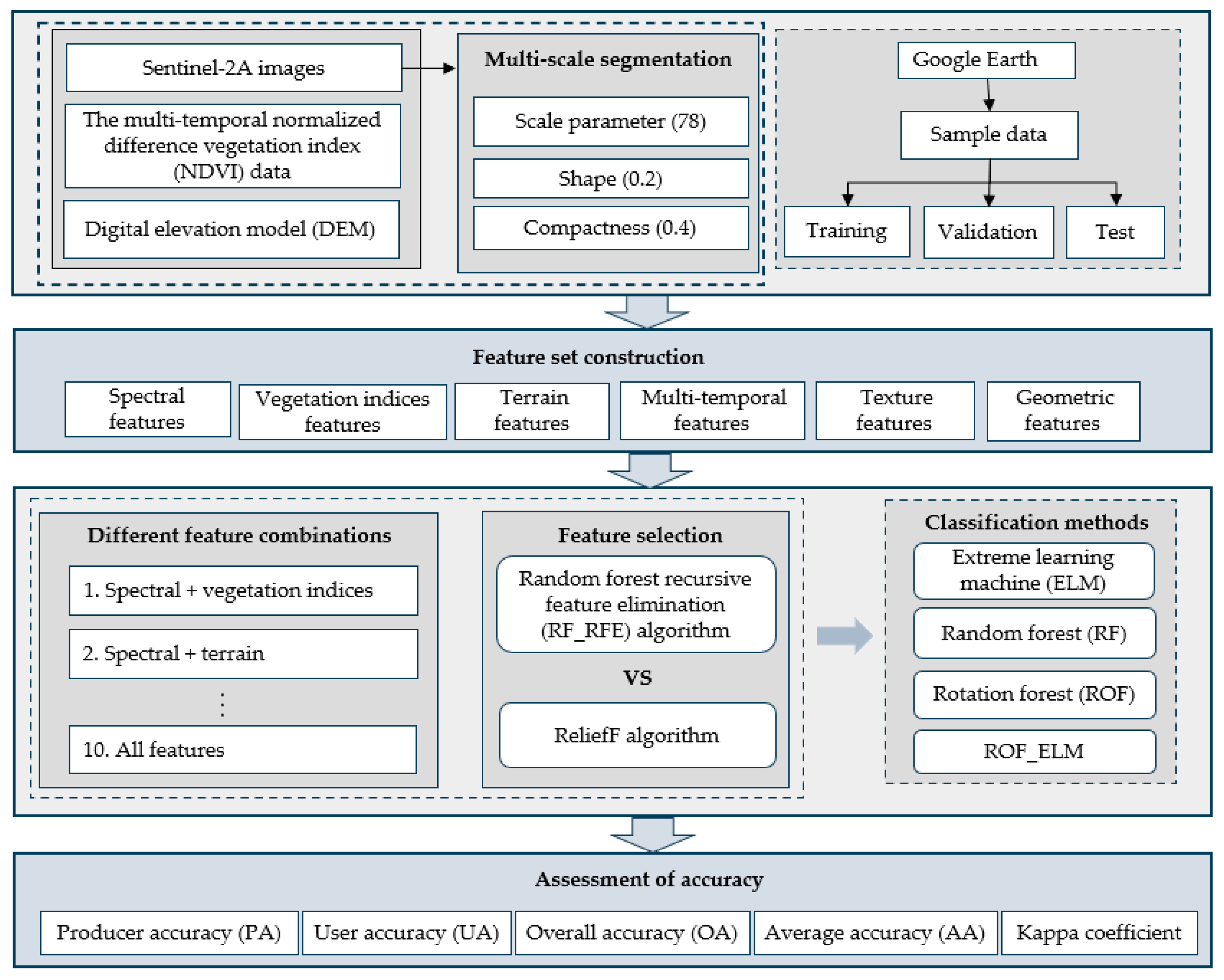
The characteristics of the study area allowed nine land cover types to be defined (Table 1), which included vegetated areas (coniferous forest, broad-leaved forest, coniferous and broad-leaved mixed forest, cultivated vegetation, shrubland, and grassland) and non-vegetated areas (bare land, built-up land, and water). All samples were selected by visual interpretation of Google Earth 7.3.6 high-resolution images. The auxiliary data selected for the sample reference include the vegetation classification data of the 2010 ecological decade [36], the global 30 m surface coverage classification data in 2020 [37], and the resource satellite 2 m resolution fusion image. The resource satellite 2 m resolution fusion image was purchased from Suzhou Zhongke Tianqi Remote Sensing Technology Co., Ltd. (Suzhou, China). The data were generated using the company’s self-developed software system based on GF-1 multispectral data. The data were collected from 2015 to 2017, covering only part of the study area. A total of 1661 samples were randomly selected according to the principle of representativeness. Of these, 1128 samples were divided into training and validation sets based on a ratio of approximately 8:2, and the remaining 533 samples were used as a test set to evaluate the final prediction results.

3. Methods

In order to achieve the fine classification of mountainous vegetation types, this study first performed image segmentation using a multi-scale segmentation method based on Sentinel-2A images to obtain ground objects. Then, the spectral, vegetation indices, terrain, texture, geometry, and multi-temporal features of each object were extracted to explore the impact of different feature combinations on mountainous vegetation type classification. Additionally, the remaining features, after removing high correlation, were subjected to feature selection using the RF_RFE and ReliefF algorithms. The classification performance of the feature combinations obtained by these two algorithms was compared. Finally, based on the optimal feature combination, the efficiency of four different machine learning algorithms, ELM, RF, ROF and ROF_ELM, in extracting mountain vegetation types was evaluated. The methodology flowchart is shown in Figure 2. The paper utilized the Python programming language to implement feature selection, mountainous vegetation type classification, and accuracy assessment.

3.1. Multi-Scale Segmentation

The workflow for object-oriented classification involves segmentation followed by classification. Segmentation refers to the process of dividing satellite images’ geographic spatial data into homogeneous regions or objects. Multi-scale segmentation is a method that starts from individual pixels and merges them bottom-up. Parameter settings include segmentation scale, shape, and compactness. The segmentation scale is one of the most important parameters, as it determines the internal heterogeneity of the segmented polygon objects [38]. In this study, the eCognition 9.1 software was used to perform multi-scale segmentation and generate image objects. The automatic segmentation scale parameter selection ESP2 tool was employed to determine the segmentation scale [39]. The values for shape and compactness parameters were determined using the control variable method, with a step size of 0.1. By continuously debugging each parameter, the segmentation scale, shape, and compactness values were set to 78, 0.2, and 0.4, respectively. Additionally, the weight of the near-infrared band was assigned a value of 2 to enhance the differentiation of vegetation types.

3.2. Feature Extraction

3.2.1. Feature Set Construction

Two additional spectral features, brightness and max.diff, were derived from the original 10 spectral bands. Brightness refers to the average reflectance of the segmented object. Max.diff indicates the maximum difference between pixels in the same object. Principal component analysis (PCA) was then applied to extract information from the preprocessed Sentinel-2A images, with the first principal component band capturing 95% of the image information. The gray-level co-occurrence matrix (GLCM) method, based on the first principal component band, was utilized to extract textural features. To enhance the discrimination between vegetation types, the soil-adjusted vegetation index (SAVI), ratio vegetation index (RVI), red-edged NIR-normalized vegetation index (REDNDVI) and difference vegetation index (DVI) were calculated based on the original spectral bands [40,41]. The terrain features were also extracted during this process, as topography influences hydrothermal conditions by directly or indirectly affecting vegetation distribution. Alongside the above features, we also introduced geometric features and multi-temporal features to explore the impact on vegetation classification. The components of different feature types are shown in Table 2.

3.2.2. Feature Optimization

The quality of feature selection greatly affects the design and performance of the classifier. There are two principles of feature selection [37]: first, ground objects should be easy to distinguish, and second that as few features as possible should be used to ensure accuracy. The paper compared and analyzed two feature selection algorithms, RelifF and RF_RFE. The ReliefF algorithm is a classical multivariate filtering feature selection method. Its core idea is to calculate the weight of features according to the correlation between features and class labels [42]. RF_RFE feature selection first obtains the importance ranking of each feature based on the RF classifier. It deletes the feature with the lowest importance score by backward iteration and then re-evaluates the importance ranking of the remaining features with the RF classifier. Repeat the steps until the feature set is empty. Finally, the optimal feature set is obtained according to the classification performance of each group of features [43].

3.3. Classification Methods

3.3.1. ELM Algorithm

The ELM algorithm is an efficient learning algorithm based on single-hidden-layer feedforward neural network (SLFN) [27]. It has a simple three-layer structure comprised of an input layer, a hidden layer, and an output layer. For a supervised learning problem containing N different samples, the training process of the ELM can be summarized as follows [44]. Firstly, the input weight matrix ω and threshold b are randomly generated based on the number of hidden layer nodes. Next, the output matrix H of the hidden layer is calculated. Finally, the weight matrix β between the hidden layer and the output layer is computed.

3.3.2. RF Algorithm

The RF algorithm, first proposed by Breiman [45], is an ensemble learning method that constructs multiple decision trees. It trains the base classifier by randomly selecting a training data set, constructing multiple classification trees, and aggregating the results of each tree to make a prediction. The RF algorithm can be implemented as follows [46]. Firstly, construct n decision trees by randomly selecting n subsets from the training sample set by replacement. Next, assume that the total number of features in each sample subset is M. Select m feature variables (m ≤ M) at all nodes of each decision tree, and count the amount of information contained in each variable in order to achieve complete splitting. Finally, summarize the results of each decision tree by using the simple majority voting method and determine the final category of prediction by the voting results.

3.3.3. ROF Algorithm

The ROF algorithm was first proposed by Rodriguez et al. [26] in 2006. It is also a multi-classifier integration model that uses decision trees and has good classification performance when applied to small and medium datasets [47]. The core of the algorithm involves processing initial data by using principal component analysis and rotation matrix methods. The processed sample data can increase the variability of the base classifier and improve classification accuracy. The ROF algorithm primarily involves the following steps. Firstly, the input training set is divided into multiple feature subsets. Each feature subset is then resampled with 75% of the data to form sample subsets. Principal component analysis is performed to calculate the coefficients for each sample subset, creating a coefficient matrix. Next, the sample subsets are multiplied with the coefficient matrix to obtain a new training set, which is used to train the base classifiers. This process is repeated L times, resulting in L-trained base classifiers. Finally, the majority voting method is applied to produce the final prediction results.

3.3.4. ROF_ELM Algorithm

The ROF_ELM algorithm is an improved model combining the ELM and ROF algorithms. It differs from the ROF algorithm in that its base classifier is ELM instead of a decision tree. The initial sample set is processed using principal component analysis and rotational transformation to obtain a new training set, which is then used as the input to the base classifier ELM. The transformed sample labels are then used as network outputs to construct multiple base classifiers. Finally, the prediction results are obtained by combining the predicted values of each base classifier [30].

3.4. Accuracy Assessment

Evaluation of the accuracy of prediction results can determine the reliability of the classification. Here, we used a confusion matrix [48,49] containing several indicators to evaluate the vegetation classification results, including producer accuracy (PA), user accuracy (UA), overall accuracy (OA), average accuracy (AA), and the kappa coefficient.

4. Results

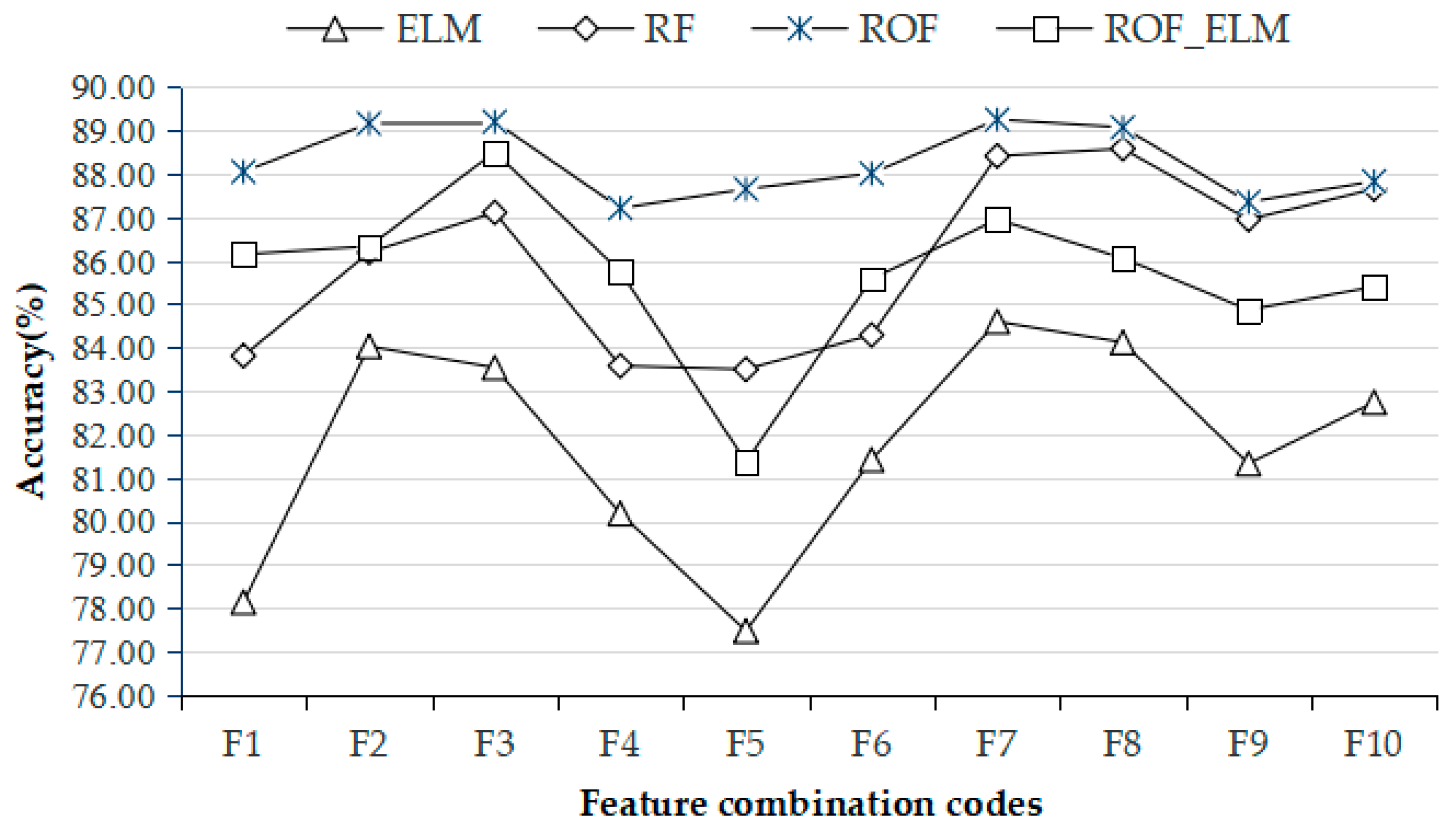
4.1. Classification Performance of Different Feature Combinations

To explore the impact of different features on mountain vegetation type classification, vegetation indices, terrain, texture, geometric, and multi-temporal features were sequentially added to the spectral features (Table 3). Different combinations of features allowed four individual classifiers to be used for model training. The average accuracy of the validation set was obtained by running the trained classifiers ten times (Figure 3). To eliminate potential bias that may arise due to changes in sample selection, all four classifiers used the same training and validation samples. Furthermore, to better compare the performance of the classifiers, we assessed the execution time of different classifiers (Table 4).
The classification accuracy of different classifiers was compared under the feature combination codes F1~F6. The ROF algorithm showed the best classification performance when only spectral features were used, with an average accuracy of 88.05%. The ROF_ELM and RF algorithms exhibited slightly lower classification performance with average accuracies of 86.15% and 83.81%, respectively. The ELM algorithm had the lowest accuracy, with an average of 78.14%. The inclusion of vegetation indices significantly improved the accuracy of each classifier. The ELM algorithm showed the largest improvement, with an accuracy increase of 5.89%, and the RF, ROF, and ROF_ELM algorithms improved by 2.38%, 1.11%, and 0.18%, respectively. When spectral and terrain features were both added to the classification, the accuracy of the RF, ROF, and ROF_ELM algorithms showed a greater improvement than increases associated with incorporating spectral and vegetation indices. In this case, the accuracy of the ELM, RF, ROF, and ROF_ELM algorithms increased by 5.40%, 3.3%, 1.15%, and 2.35%, respectively. The addition of textural features resulted in a decrease in accuracy for the RF, ROF, and ROF_ELM algorithms, with decreases of 0.23%, 0.84%, and 0.4%, respectively, compared to using only spectral features. However, the ELM algorithm’s classification accuracy improved by 2.04%. The addition of geometric features decreased the accuracy of the ELM, RF, ROF, and ROF_ELM algorithms by 0.66%, 0.31%, 0.40%, and 4.78%, respectively. Incorporating multi-temporal features in the classification improved the accuracy of the ELM and RF algorithms by 3.28% and 0.48%, respectively, compared to using only spectral features. However, the accuracy of the ROF and ROF_ELM algorithms decreased by 0.04% and 0.57%, respectively.
These results indicated that terrain features have the most significant impact on mountain vegetation type classification, followed by vegetation indices, multi-temporal features, texture features, and geometric features.
Based on the classification performance of different types of features obtained in the previous step, the features of each type were combined and added to the classification in turn (feature combination codes F7~F10). The inclusion of spectral features, vegetation indices, and terrain features in the classification caused the ELM, ROF, and ROF_ELM algorithms to reach their highest recorded accuracies of 84.60%, 89.25%, and 86.95%, respectively. By contrast, the RF algorithm achieved its highest accuracy of 88.58% when multi-temporal features were added (i.e., feature combination code F8). However, when textural features and geometric features were sequentially added (i.e., feature combination codes F9 and F10), the accuracy of the four different classifiers showed a declining trend when compared with feature combination code F8.
In summary, without considering data redundancy, the combination of spectral features, vegetation indices, and terrain features was found to be more likely to achieve accurate classification of mountain vegetation types. In the comparison of the execution time of different classifiers, it was observed that ROF_ELM took the longest time, followed by ROF, RF, and ELM.

4.2. Comparison of Different Feature Optimization Algorithms

The features with a correlation value greater than 0.9 were removed, and the remaining 35 features were used by the RF_RFE and RliefF algorithms for feature selection (Figure 4). The 12 features were retained based on the RF_RFE algorithm. To better compare the effectiveness of the two feature selection algorithms, the ReliefF algorithm also retained the top 12 features based on their weight values. Only a fraction of terrain features, spectral features, vegetation index features and multi-temporal features were retained in the RF_RFE and ReliefF algorithm results, while the ReliefF algorithm retained geometric features that were not included in the RF_RFE algorithm, and texture features were not retained by either feature-selection algorithm.
A comparison of the accuracy of different classifiers based on different feature optimization algorithms is given in Table 5. The feature combination based on the RF_RFE algorithm outperformed the ReliefF algorithm in classifying mountain vegetation types. The classification accuracy of the ELM, ROF, and ROF_ELM algorithms improved after RF_RFE feature selection. The ROF algorithm achieved the highest accuracy of 89.65%, followed by the ELM and ROF_ELM algorithms with accuracies of 86.50% and 89.38%, respectively. However, the RF algorithm’s accuracy after feature selection was 87.30%, which did not show improvement compared to the feature combination code F8.
In summary, after eliminating data redundancy, the utilization of the RF_RFE feature selection algorithm further improved the accuracy of mountain vegetation type classification. The retained feature types mainly included spectral, terrain and vegetation indices features.

4.3. Visual Comparison of Mountain Vegetation Mapping Based on Different Classifiers

Based on the optimal feature combination extracted by the RF_RFE algorithm, the distribution and area statistics of different vegetation types in Jiuzhaigou County obtained by various classifiers showed minimal variation (Figure 5 and Figure 6). The majority of Jiuzhaigou County was covered by vegetation, with shrubland and grassland being the two largest vegetation types in terms of area. Shrubland and cultivated vegetation were mainly observed along the perimeter of the town, while grassland was predominantly located in the western part of the study area at high elevations. Coniferous forests were primarily found at high elevations in the central and western regions. Coniferous and broad-leaved mixed forests and broad-leaved forests were scattered throughout the entire area. Non-vegetated areas were mainly concentrated in low-lying valleys and plateau regions covered by perennial snow and ice.
To further investigate the classification differences between each classifier, a detailed study was conducted in a selected local area of Jiuzhaigou County (Figure 7). Upon examining the details, it was observed that the ROF_ELM algorithm misclassified some water areas by categorizing them as broad-leaved forests. Within the red ellipse, the ROF algorithm outperformed the other classifiers by accurately identifying a non-vegetated region. The ELM and ROF_ELM algorithms showed similar recognition of coniferous forests, as indicated slightly north of the red rectangle. The RF and ROF algorithms demonstrated similar identification of coniferous and broad-leaved mixed forests within the red rectangle. This comparative analysis revealed that integrated learning models consisting of the same base classifier exhibited similar classification performance.

4.4. Assessing the Accuracy of the Classification Results

The accuracy of the four classifiers was analyzed together (Table 6). The UA and PA values of the coniferous forest were between 84.09% and 92.68%, and the UA and PA values of the coniferous and broad-leaved mixed forest were relatively low, with values between 46.94% and 85.19%. The UA values exceeded the PA values in all four classification algorithms for coniferous forest and coniferous and broad-leaved mixed forest, which indicated that both vegetation types are more likely to be missed during classification than to be misclassified.
The UA and PA values of broad-leaved forest and shrubland were within the ranges 75.00%–93.40% and 79.27%–90.00%, respectively. The PA values exceeded the UA values for broad-leaved forest and shrubland in all four classification algorithms, indicating that misclassification was more likely to occur for those vegetation types. Broad-leaved forest and shrubland were easily misclassified into coniferous and broad-leaved mixed forest.
The UA and PA values of grassland, cultivated vegetation and other non-vegetation types were within the ranges 88.46%–98.86%, 66.67%–100.00%, and 79.17%–100.00%, respectively. For these types of ground object recognition, the PA and UA values associated with different classifiers showed no clear relationships.
Compared to the classification performance of the four classifiers, the ROF algorithm performed best, with OA, AA, and kappa coefficient of 89.68%, 88.48%, and 0.879, respectively. The ROF_ELM algorithm ranked second, with OA, AA, and kappa coefficient of 87.05%, 87.61%, and 0.849, respectively. The RF algorithm ranked third, with OA, AA, and kappa coefficients of 86.12%, 86.55%, and 0.837, respectively. The ELM algorithm performed relatively lower, with an OA of 84.62%, an AA of 85.11%, and a kappa coefficient of 0.820.
Overall, the ROF algorithm was superior to the other three classification algorithms in distinguishing coniferous forest, broad-leaved forest, shrubland and grassland. The RF algorithm performed well in identifying the vegetation types of coniferous and broad-leaved mixed forests. The ROF_ELM algorithm demonstrated the best recognition performance for cultivated vegetation.

5. Discussion

5.1. The Influence of Incorporating Different Features on Mountain Vegetation Type Classification

Our study has demonstrated that the inclusion of vegetation indices and terrain features significantly improves the accuracy of mountain vegetation type classification, which is consistent with the findings of Zhou and Yang et al. [12,50]. However, the addition of textural and geometric features causes the classification accuracy to slightly decrease, which is different from the conclusions of other workers [13]. This discrepancy may be attributed to the relatively lower importance of textural and geometric features compared to spectral features in mountain vegetation type classification, resulting in data redundancies.
Compared to the ReliefF algorithm, the RF_RFE algorithm yielded better results in feature selection for mountain vegetation type classification. The presence of DEM, B11, DVI, SAVI, RVI, NDVI_summer, Stdv_b4, and Slope in both feature selection methods indicates that infrared bands, topographic features and vegetation index features have significant advantages in mountain vegetation type identification [11]. However, among the multi-temporal features, only summer NDVI was retained. This could be attributed to the wide temporal span of the selected multi-temporal features, which may not effectively capture the phenological information that reflects different vegetation types. Furthermore, mountains are susceptible to cloudy and rainy conditions, making it difficult for the Sentinel-2A satellite to construct a complete time series of cloud-free images. In future research, it would be beneficial to incorporate multi-temporal spectral data or multi-source data, as well as integrate additional data, such as hydrological and road network information, into the classification process [51,52].

5.2. The Performance of Different Classifiers in Mountain Vegetation Type Recognition

The four different machine learning algorithms used in the study exhibited similar performance in identifying vegetation types in Jiuzhaigou County, with minor differences in the area estimation. Coniferous forest, cultivated vegetation, grassland and non-vegetation types were effectively distinguished. The recognition accuracy of broad-leaved forest and shrubland was slightly lower, while the recognition of coniferous and broad-leaved mixed forest was poor. The main reason is that coniferous and broad-leaved mixed forest, broad-leaved forest and shrub have little difference in spectrum and auxiliary characteristics, which makes them prone to mutual misclassification [53].
The difference between the ROF and RF algorithms lies in whether or not the initial feature data are processed. The ROF algorithm achieved higher recognition accuracy for most vegetation types, and the overall accuracy was better than the RF algorithm, which is consistent with the findings of Liang et al. [54]. It indicates that increasing the dissimilarity between input features can improve classification accuracy.
The results of testing local vegetation type recognition by different classifiers showed that RF and ROF algorithms performed similarly, as did the ELM and ROF_ELM algorithms. This indicates that the classification performance of ensemble learning algorithms is highly influenced by the base classifiers. Different base classifiers often have separate advantages in distinguishing vegetation categories. In this paper, only the classification accuracy of ensemble learning algorithms using ELM and decision trees as base classifiers was compared and analyzed. In future research, different types of base classifiers should be introduced for comparative study, or otherwise, the integration of different base classifiers could be used to explore how algorithms for mountain vegetation type classification could be improved.
The improved ROF_ELM classifier used in the study did not outperform the ROF classifier, which indicates that there is no universal classifier that is perfectly suited for all classification scenarios. The most appropriate classifier should thus be selected according to the characteristics of the studied scenario.

6. Conclusions

The research demonstrated that incorporating additional features, such as spectral, vegetation indices, and terrain features, can enhance the accuracy of vegetation type classification. However, the inclusion of textural and geometric features resulted in data redundancy and hindered the accurate identification of vegetation types. Nevertheless, by performing feature selection, the redundancy in data can be reduced, leading to improved classification accuracy for mountain vegetation types. The RF_RFE algorithm exhibited superior performance compared to the ReliefF algorithm in the feature selection process for mountain vegetation type classification.
In the recognition of mountain vegetation types, given the limited feature data and classifier performance, enhancing the dissimilarity between data through some data processing methods is an important approach to improve classification accuracy. The performance of ensemble classifiers is significantly influenced by the base classifier. Classification algorithms integrated by using the same base classifier often showed similar classification performance.
The four machine learning algorithms studied here achieved a good level of classification with an overall accuracy greater than 84.62% and an average accuracy greater than 85.11% in Jiuzhaigou County. The ROF algorithm showed the highest overall classification accuracy of 89.68%, an average accuracy of 88.48%, and a kappa coefficient of 0.879.

Author Contributions

Conceptualization, F.L.; Methodology, X.F., X.Z. and F.L.; Software, X.F. and X.Z.; Validation, X.F.; Formal analysis, X.F.; Investigation, X.Z.; Resources, F.L.; Data curation, X.F.; Writing—original draft, X.F.; Writing—review & editing, W.Z. and Y.H.; Visualization, X.F.; Supervision, W.Z.; Project administration, W.Z.; Funding acquisition, W.Z. All authors have read and agreed to the published version of the manuscript.

Funding

This research was funded by [The National Science and Technology Basic Resource Investigation Program] grant number [2017FY100900].

Institutional Review Board Statement

Not applicable.

Informed Consent Statement

Not applicable.

Data Availability Statement

Not applicable.

Conflicts of Interest

The authors declare no conflict of interest.

References

  1. Chen, Y.; Mo, D.; Yan, E. Analysis on Topographic Effects of Commonly Used Vegetation Indices in Complex Mountain Area Based on Sentinel-2 Data. Chin. J. Ecol. 2022, 42, 956–965. [Google Scholar]
  2. Wu, T.; Luo, J.; Gao, L.; Sun, Y.; Dong, W.; Zhou, Y.N.; Liu, W.; Hu, X.; Xi, J.; Wang, C.; et al. Geo-Object-Based Vegetation Mapping via Machine Learning Methods with an Intelligent Sample Collection Scheme: A Case Study of Taibai Mountain, China. Remote Sens. 2021, 13, 249. [Google Scholar] [CrossRef]
  3. Yao, Y.H.; Suonan, D.Z.; Zhang, J.Y. Compilation of 1:50,000 vegetation type map with remote sensing images based on mountain altitudinal belts of Taibai Mountain in the North-South transitional zone of China. J. Geogr. Sci. 2020, 30, 267–280. [Google Scholar] [CrossRef]
  4. Guo, Y.; Wu, T.; Luo, J.; Shi, H.; Hao, L. Remote Sensing Mapping of Mountain Vegetation via Uncertainty-based Iterative Optimization. Geo-Inf. Sci. 2022, 24, 1406–1419. [Google Scholar]
  5. Cai, Y.T.; Zhang, M.; Lin, H. Estimating the Urban Fractional Vegetation Cover Using an Object-Based Mixture Analysis Method and Sentinel-2 MSI Imagery. IEEE J. Sel. Top. Appl. Earth Obs. Remote Sens. 2020, 13, 341–350. [Google Scholar] [CrossRef]
  6. Zheng, Y.; Wu, J.; Wang, A.; Chen, J. Object- and pixel-based classifications of macroalgae farming area with high spatial resolution imagery. Geocarto Int. 2018, 33, 1048–1063. [Google Scholar] [CrossRef]
  7. Nyamjargal, E.; Amarsaikhan, D.; Munkh-Erdene, A.; Battsengel, V.; Bolorchuluun, C. Object-based classification of mixed forest types in Mongolia. Geocarto Int. 2020, 35, 1615–1626. [Google Scholar] [CrossRef]
  8. Guo, Y.; Yu, X.; Jiang, D.; Wang, S.; Jiang, X. Study on Forest Classification Based on Object Oriented Techniques. Geo-Inf. Sci. 2012, 14, 514–522. [Google Scholar] [CrossRef]
  9. Agarwal, S.; Vailshery, L.S.; Jaganmohan, M.; Nagendra, H. Mapping Urban Tree Species Using Very High Resolution Satellite Imagery: Comparing Pixel-Based and Object-Based Approaches. ISPRS Int. J. Geo-Inf. 2013, 2, 220–236. [Google Scholar] [CrossRef] [Green Version]
  10. Qu, L.A.; Chen, Z.; Li, M.; Zhi, J.; Wang, H. Accuracy Improvements to Pixel-Based and Object-Based LULC Classification with Auxiliary Datasets from Google Earth Engine. Remote Sens. 2021, 13, 453. [Google Scholar] [CrossRef]
  11. Dorren, L.K.A.; Maier, B.; Seijmonsbergen, A.C. Improved Landsat-based forest mapping in steep mountainous terrain using object-based classification. For. Ecol. Manag. 2003, 183, 31–46. [Google Scholar] [CrossRef]
  12. Zhou, X.; Zhou, W.; Li, F.; Shao, Z.; Fu, X. Vegetation Type Classification Based on 3D Convolutional Neural Network Model: A Case Study of Baishuijiang National Nature Reserve. Forests 2022, 13, 906. [Google Scholar] [CrossRef]
  13. Ning, L.; Zhang, X. A Preliminary Study on Vegetation Classification based on Texture Information of Landsat-8 Images. J. Cent. South Univ. For. Technol. 2014, 34, 60–64. [Google Scholar] [CrossRef]
  14. Yang, D.; Li, C.; Li, B. Forest Type Classification Based on Multi-temporal Sentinel-2A/B Imagery Using U-Net Model. For. Res. 2022, 35, 103–111. [Google Scholar] [CrossRef]
  15. Chen, J.; Li, H.; Liu, Y.; Chang, Z.; Han, W.; Liu, S. Remote sensing recognition of agricultural crops based on Sentinel—2 data with multi—Feature optimization. Remote Sens. Nat. Resour. 2023, 1–9. Available online: http://kns.cnki.net/kcms/detail/10.1759.P.20230531.0953.006.html (accessed on 1 July 2023).
  16. Zhou, X.; Zheng, L.; Huang, H. Classification of Forest Stand Based on Multi-Feature Optimization of UAV Visible Light Remote Sensing. Sci. Silvae Sin. 2021, 57, 24–36. [Google Scholar]
  17. Liu, J.; Li, L.; Ren, C.; Mao, D.; Zhang, B. Information Extraction of Coastal Wetlands in Yellow River Estuary by Optimal Feature-based Random Forest Model. Wetl. Sci. 2018, 16, 97–105. [Google Scholar] [CrossRef]
  18. Zhang, D.; Yang, Y.; Huang, L.; Yang, Q.; She, B.; Hong, Q.; Jiang, F. Extraction of soybean planting areas combining Sentinel-2 images and optimized feature model. Trans. Chin. Soc. Agric. Eng. 2021, 37, 110–119. [Google Scholar]
  19. Thanh Noi, P.; Kappas, M. Comparison of Random Forest, k-Nearest Neighbor, and Support Vector Machine Classifiers for Land Cover Classification Using Sentinel-2 Imagery. Sensors 2018, 18, 18. [Google Scholar] [CrossRef] [Green Version]
  20. Zhang, Z.; Zhang, Z.; Guo, Y.; Tao, G.; Ou, X. Mountain vegetation mapping using remote sensing. J. Yunnan Univ. (Nat. Sci. Ed.) 2013, 35, 416–427. [Google Scholar]
  21. Du, Z.; Ma, W.; Zhou, Q.; Chen, H.; Deng-zeng, Z.; Liu, J. Research progress of vegetation recognition methods based on remote sensing technology. Ecol. Sci. 2022, 41, 222–229. [Google Scholar] [CrossRef]
  22. Yang, C.; Wu, G.; Li, Q.; Qang, J.; Qu, L.; Ding, K. Research Progress on Remote Sensing Classification of Vegetation. Geogr. Geo-Inf. Sci. 2018, 34, 24–32. [Google Scholar]
  23. Belgiu, M.; Drăguţ, L. Random forest in remote sensing: A review of applications and future directions. ISPRS J. Photogramm. Remote Sens. 2016, 114, 24–31. [Google Scholar] [CrossRef]
  24. Yu, Y.; Gao, H.; Tao, Y.; Wang, S. A Review of Hyperspectral Remote Sensing Image Classification Based on Ensemble Learning. Geomat. Spat. Inf. Technol. 2023, 46, 49–52+60. [Google Scholar]
  25. Chi, M.; Kun, Q.; Benediktsson, J.A.; Feng, R. Ensemble Classification Algorithm for Hyperspectral Remote Sensing Data. IEEE Geosci. Remote Sens. Lett. 2009, 6, 762–766. [Google Scholar] [CrossRef]
  26. Rodriguez, J.J.; Kuncheva, L.I. Rotation forest: A new classifier ensemble method. IEEE Trans. Pattern Anal. Mach. Intell. 2006, 28, 1619–1630. [Google Scholar] [CrossRef]
  27. Huang, G.B.; Zhu, Q.Y.; Siew, C.K. Extreme learning machine: Theory and applications. Neurocomputing 2006, 70, 489–501. [Google Scholar] [CrossRef]
  28. Liu, T.; Fan, Q.; Kang, Q.; Niu, L. Extreme Learning Machine Based on Firefly Adaptive Flower Pollination Algorithm Optimization. Processes 2020, 8, 1583. [Google Scholar] [CrossRef]
  29. Ding, S.; Zhao, H.; Zhang, Y.; Xu, X.; Nie, R. Extreme learning machine: Algorithm, theory and applications. Artif. Intell. Rev. 2015, 44, 103–115. [Google Scholar] [CrossRef]
  30. Han, M.; Liu, B. An Improved Rotation Forest Classification Algorithm. J. Electron. Inf. Technol. 2013, 35, 2896–2900. [Google Scholar] [CrossRef]
  31. Du, X. A Large Sample Ensemble Classification Algorithm Based on Rotation-forest-extreme Learning Machine classifier. Sci. Technol. Eng. 2018, 18, 231–235. [Google Scholar]
  32. Tang, Y.; Wang, Z. Quantitative Analysis of Soil Erosion after Earthquake in Jiuzhaigou County Based on Rulse. Chem. Eng. Des. Commun. 2021, 47, 86–87+100. [Google Scholar]
  33. Hao, Y.; Jiang, H.; Wang, J.; Jin, J.; Ma, Y. Vegetation Landscape Change Pattern and Habitats Fragmentation in Jiuzhaigou Nature Reserve. Sci. Geogr. Sin. 2009, 29, 886–892. [Google Scholar]
  34. Fu, X.; Zhou, W.; Zhou, X.; Li, F. Application of Machine Learning in Vegetation Interpretation of Natural Protected Areas in Jiuzhaigou County. Nat. Prot. Areas 2023, 3, 53–65. [Google Scholar]
  35. Ghayour, L.; Neshat, A.; Paryani, S.; Shahabi, H.; Shirzadi, A.; Chen, W.; Al-Ansari, N.; Geertsema, M.; Pourmehdi Amiri, M.; Gholamnia, M.; et al. Performance Evaluation of Sentinel-2 and Landsat 8 OLI Data for Land Cover/Use Classification Using a Comparison between Machine Learning Algorithms. Remote Sens. 2021, 13, 1349. [Google Scholar] [CrossRef]
  36. Ouyang, Z.; Wang, Q.; Zheng, H.; Zhang, F.; Hou, P. National Ecosystem Survey and Assessment of China (2000–2010). Bull. Chin. Acad. Sci. 2014, 29, 426–466. [Google Scholar]
  37. Zhang, X.; Liu, L.Y.; Chen, X.D.; Gao, Y.; Xie, S.; Mi, J. GLC_FCS30: Global land-cover product with fine classification system at 30 m using time-series Landsat imagery. Earth Syst. Sci. Data 2021, 13, 2753–2776. [Google Scholar] [CrossRef]
  38. Wang, Y.; Wang, Y.; Li, M.; Liang, D. Estimation Method of Phyllostachys Edulis Forest Canopy Density Based on UAV Visible Image. J. Zhejiang A F Univ. 2022, 39, 981–988. [Google Scholar]
  39. Fu, B.; Liu, M.; He, H.; Lan, F.; He, X.; Liu, L.; Huang, L.; Fan, D.; Zhao, M.; Jia, Z. Comparison of optimized object-based RF-DT algorithm and SegNet algorithm for classifying Karst wetland vegetation communities using ultra-high spatial resolution UAV data. Int. J. Appl. Earth Obs. Geoinf. 2021, 104, 102553. [Google Scholar] [CrossRef]
  40. Ahmadi, K.; Mahmoodi, S.; Pal, S.C.; Saha, A.; Chowdhuri, I.; Nguyen, T.T.; Jarvie, S.; Szostak, M.; Socha, J.; Thai, V.N. Improving species distribution models for dominant trees in climate data-poor forests using high-resolution remote sensing. Ecol. Model. 2023, 475, 110190. [Google Scholar] [CrossRef]
  41. Wang, L.; Kong, Y.; Yang, X.; Xu, Y.; Liang, L.; Wang, S. Classification of land use in farming areas based on feature optimization random forest algorithm. Trans. Chin. Soc. Agric. Eng. 2020, 36, 244–250. [Google Scholar]
  42. Reyes, O.; Morell, C.; Ventura, S. Scalable extensions of the ReliefF algorithm for weighting and selecting features on the multi-label learning context. Neurocomputing 2015, 161, 168–182. [Google Scholar] [CrossRef]
  43. Mahmoudian, M.; Venalainen, M.S.; Klen, R.; Elo, L.L. Stable Iterative Variable Selection. Bioinformatics 2021, 37, 4810–4817. [Google Scholar] [CrossRef] [PubMed]
  44. Xu, H.; Ma, C.; Feng, H. A Thrust Allocation Method Based on Extreme Learning Machine. J. Huazhong Univ. Sci. Technol. (Nat. Sci. Ed.) 2021, 49, 34–39+70. [Google Scholar] [CrossRef]
  45. Breiman, L. Random forests. Mach. Learn. 2001, 45, 5–32. [Google Scholar] [CrossRef] [Green Version]
  46. Yang, Y.; Liu, B.; Zhang, H.; Zhang, W. Research on GF-2 Image Classification Based on Feature Optimization Random Forest Algorithm. Spacecr. Recovery Remote Sens. 2022, 43, 115–126. [Google Scholar]
  47. Wang, Q. Data Analysis of College Practice Teaching Based on Rotation Forests and LightGBM Classification algorithm. Master’s Thesis, Jilin University, Changchun, Chima, 2020. [Google Scholar]
  48. Congalton, R.G. A Review of Assessing the Accuracy of Classifications of Remotely Sensed Data. Remote Sens. Environ. 1991, 37, 35–46. [Google Scholar] [CrossRef]
  49. Stehman, S.V. Selecting and interpreting measures of thematic classification accuracy. Remote Sens. Environ. 1997, 62, 77–89. [Google Scholar] [CrossRef]
  50. Yang, X.; Zhang, W.; Sun, B.; Gao, Z.; Li, Y.; Wang, H. Recognition of Vegetation Types in Hulunbuir Sandy Land and Its Surrounding Areas Based on GEE Cloud Platform and Sentinel-2 Time Series Data. Remote Sens. Technol. Appl. 2022, 37, 982–992. [Google Scholar]
  51. Yang, D.; Zhou, Y.; Yang, X.; Gao, L.; Feng, L. Vegetation Mapping in Taibai Mountain Area Supported by LSTM with Time Series Sentinel-1A Data. J. Geo-Inf. Sci. 2020, 22, 2445–2455. [Google Scholar]
  52. Pouliot, D.; Latifovic, R.; Zabcic, N.; Guindon, L.; Olthof, I. Development and assessment of a 250m spatial resolution MODIS annual land cover time series (2000–2011) for the forest region of Canada derived from change-based updating. Remote Sens. Environ. 2014, 140, 731–743. [Google Scholar] [CrossRef]
  53. You, J.; Li, M.; Fan, W.; Quan, Y.; Wang, B.; Mo, Z.; Zhu, Z. Stand Type Identification Based on Hyperspectral and LiDAR Data. Sci. Silvae Sin. 2021, 57, 119–129. [Google Scholar]
  54. Liang, X.; Zhao, Y.; Zhen, Z.; Wei, Q. Forest Vegetation Classification of Landsat-8 Based on Rotation Forest. J. Northeast For. Univ. 2017, 45, 39–48. [Google Scholar] [CrossRef]
Figure 1. An overview map of the study area showing the distribution of samples.
Forests 14 01624 g001
Figure 2. Methodology flowchart of this study.
Forests 14 01624 g002
Figure 3. Vegetation type classification accuracy for different feature combinations based on four machine learning algorithms.
Forests 14 01624 g003
Figure 4. Feature selection results and feature weights based on different feature selection algorithms. (a) RF_RFE, (b) ReliefF.
Forests 14 01624 g004
Figure 5. Vegetation mapping in Jiuzhaigou County based on the ELM, RF, ROF, and ROF_ELM algorithms.
Forests 14 01624 g005
Figure 6. Vegetation type area statistics in Jiuzhaigou County based on the ELM, RF, ROF, and ROF_ELM algorithms (1: coniferous forest, 2: broad-leaved forest, 3: coniferous and broad-leaved mixed forest, 4: shrubland, 5: grassland, 6: water, 7: built-up land, 8: bare land, 9: cultivated vegetation).
Forests 14 01624 g006
Figure 7. Comparison of local vegetation classification results using the ELM, RF, ROF, and ROF_ELM algorithms.
Forests 14 01624 g007
Table 1. Sample numbers and codes for each land cover category.
CodeTypesSamplesDescription
1Coniferous forest238The forest dominated by cone-bearing trees, such as pine or spruce.
2Broad-leaved forest314The forest dominated by broad-leaved trees, such as oaks or maples.
3Coniferous and broad-leaved mixed forest119The forest comprising a combination of both coniferous and broad-leaved trees.
4Shrubland224Area covered by dense growths of low, woody plants.
5Grassland324Open land dominated by grasses and other herbaceous plants.
6Water72Areas covered by bodies of water, such as lakes, rivers, or ponds.
7Built-up land114Land used for urban development, with buildings and infrastructure.
8Bare land182Land without any significant vegetation cover.
9Cultivated vegetation74Land used for agriculture or cultivated crops.
Total 1661
Table 2. The composition of the set of feature variables (SAVI, RVI, REDNDVI and DVI in the table are short for soil-adjusted vegetation index, ratio vegetation index, red-edged NIR-normalized vegetation index and difference vegetation index, respectively).
Type of FeatureVariable NameTotal Number of Variables
Spectral featuresMean, standard deviation, brightness, max.diff22
Vegetation indicesSAVI, RVI, REDNDVI, DVI4
Terrain featuresDEM, slope, aspect3
Texture featuresHomogeneity, contrast, dissimilarity, correlation, main direction, entropy, standard variance, angular second moment8
Geometric featuresMain direction, shape index, compactness, roundness, border index, asymmetry, elliptic fit, density, rectangular fit, radius of smallest/largest enclosing ellipse11
Multi-temporal featuresNDVI_spring, NDVI_summer, NDVI_autumn, NDVI_winter4
Table 3. Different feature combinations and numbers.
CodeFeature CombinationTotal Number of Features
F1Spectral22
F2Spectral + vegetation indices26
F3Spectral + terrain25
F4Spectral + texture30
F5Spectral + geometric33
F6Spectral + multi-temporal26
F7Spectral + terrain + vegetation indices29
F8Spectral + terrain + vegetation indices + multi-temporal33
F9Spectral + terrain + vegetation indices + multi-temporal + texture41
F10Spectral + terrain + vegetation indices + multi-temporal + texture + geometric52
Table 4. Execution time of different classifiers based on different feature combinations.
CodeExecution Time/s
ELMRFROFROF_ELM
F10.5324.0192.77246.05
F20.7225.9589.01273.92
F30.8525.2786.03310.68
F40.4825.8792.35263.75
F50.3225.4293.11239.04
F60.6325.4990.05263.59
F70.5330.1794.96294.46
F80.9125.5590.06270.18
F90.4624.93104.73321.49
F100.6725.5891.63343.42
Table 5. Comparison of the accuracy of different classifiers based on the RF_RFE and ReliefF feature selection algorithms.
AlgorithmELMRFROFROF_ELM
Accuracy (%)Time/sAccuracy (%)Time/sAccuracy (%)Time/sAccuracy (%)Time/s
RF_RFE86.500.4987.3017.3389.6580.5989.38209.34
ReliefF84.380.3986.9016.5588.4164.3886.86216.45
Table 6. Comparison of vegetation classification accuracy for different classifiers based on optimal feature combination (1: coniferous forest, 2: broad-leaved forest, 3: coniferous and broad-leaved mixed forest, 4: shrubland, 5: grassland, 6: water, 7: built-up land, 8: bare land, 9: cultivated vegetation).
AlgorithmELMRFROFROF_ELM
PA (%)UA (%)PA (%)UA (%)PA (%)UA (%)PA (%)UA (%)
184.0991.3686.3692.6892.0595.2986.3692.68
282.0880.5690.5775.0093.4077.9584.9178.26
357.1466.6755.1079.4146.9485.1957.1471.79
483.7579.7681.2579.2790.0086.7588.7583.53
595.8388.4690.6294.5798.8697.9496.8892.08
679.1790.4887.5095.4587.5095.4587.5095.45
790.9193.7596.9788.8996.9788.8993.9493.94
893.02100.0097.67100.0097.67100.0093.0297.56
9100.0066.6792.8686.6792.8692.86100.0093.33
OA (%)84.6286.1289.6887.05
AA (%)85.1186.5588.4887.61
Kappa0.8200.8370.8790.849
Disclaimer/Publisher’s Note: The statements, opinions and data contained in all publications are solely those of the individual author(s) and contributor(s) and not of MDPI and/or the editor(s). MDPI and/or the editor(s) disclaim responsibility for any injury to people or property resulting from any ideas, methods, instructions or products referred to in the content.

