

Empirical Comparison of Supervised Learning Methods for Assessing the Stability of Slopes Adjacent to Military Operation Roads
 , , ,
, , ,
Abstract
:1. Introduction
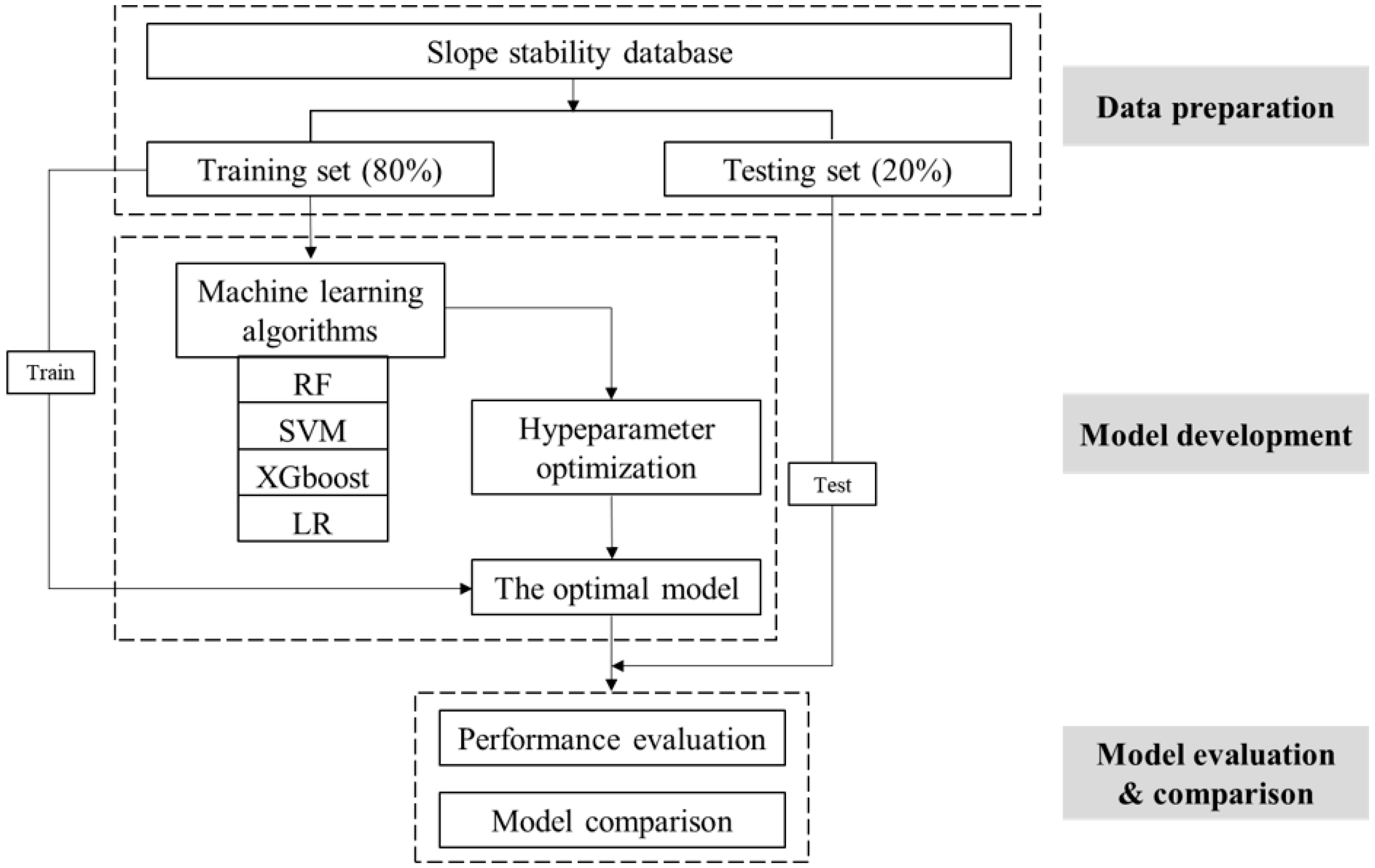
2. Materials and Methods
2.1. Investigated Data
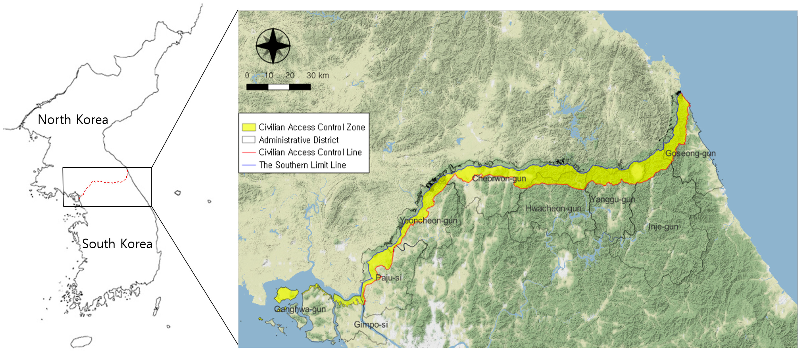
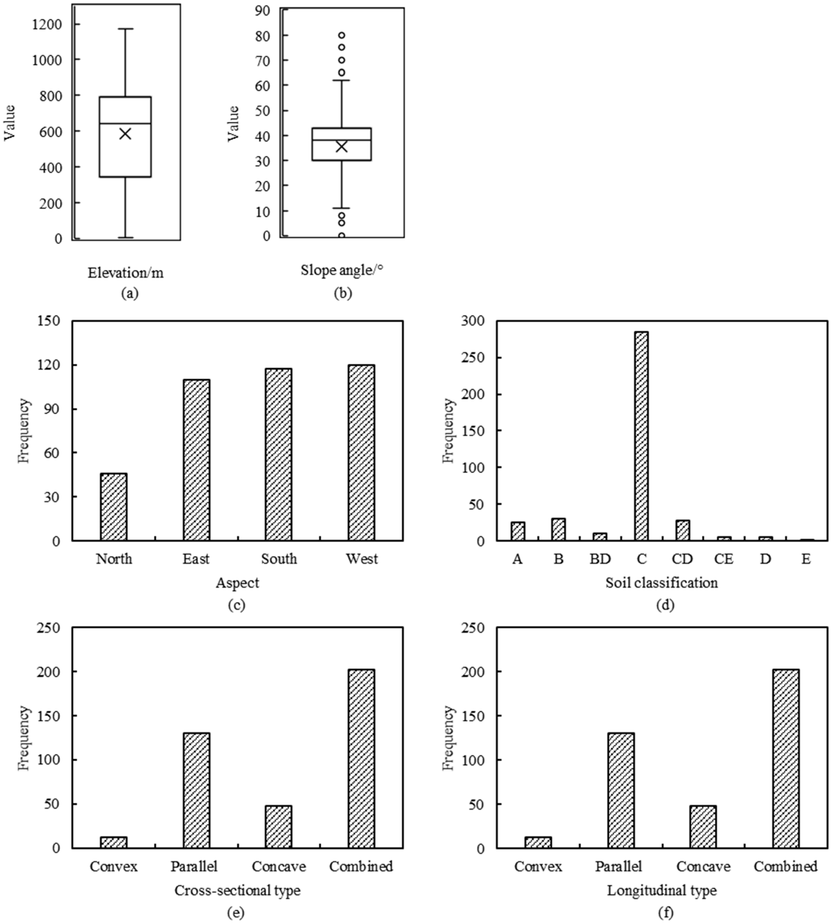
2.1.1. Slope Conditions
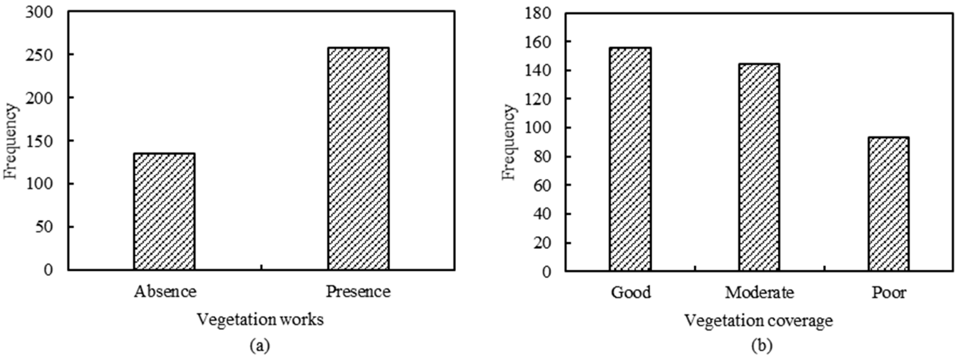
2.1.2. Vegetation Conditions
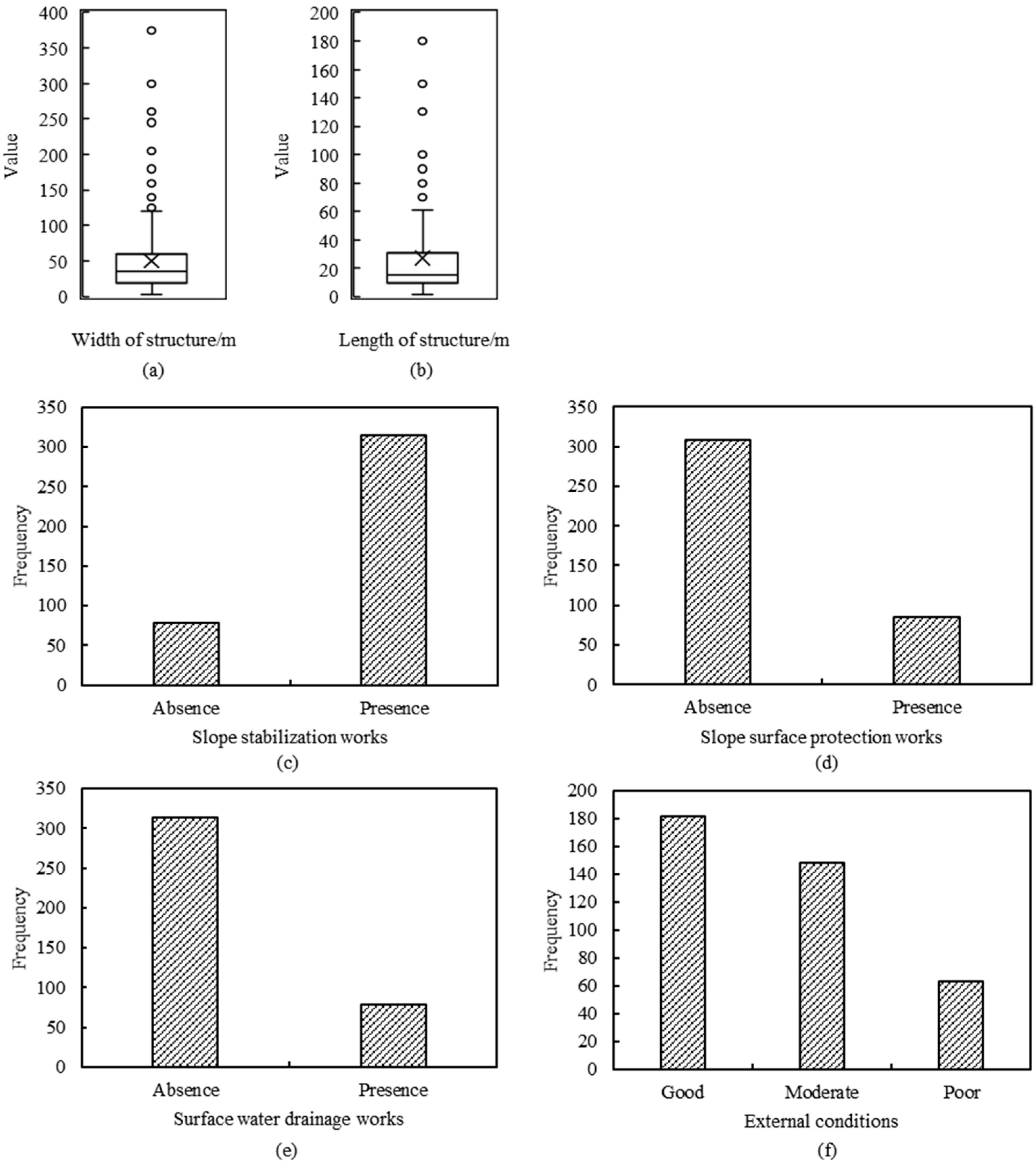
2.1.3. Structure Conditions
2.2. Data Processing
2.3. Methodology
2.3.1. Discrimination Methods
- Random forest (RF)
- 2.
- Support vector machine (SVM)
- 3.
- Extreme gradient boosting (XGBoost)
- 4.
- Logistic regression (LR)
2.3.2. Parameter Optimization
2.3.3. Performance Metrics
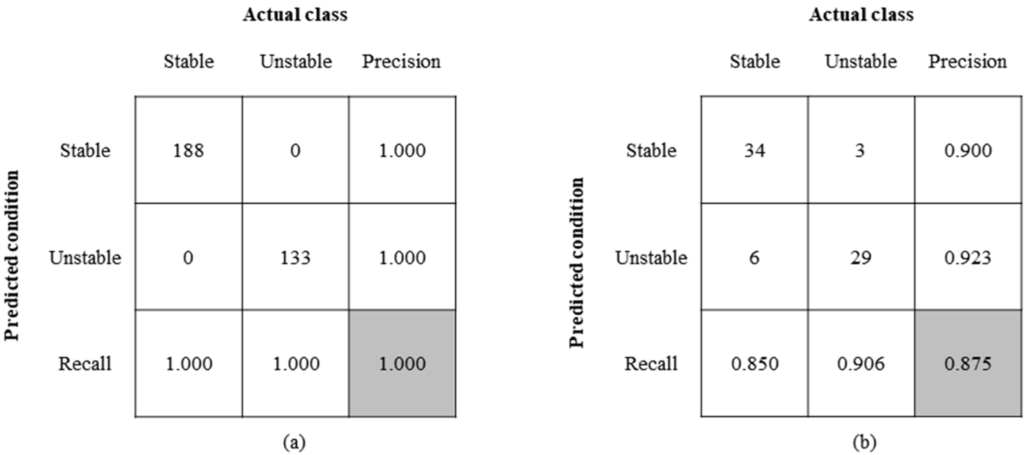
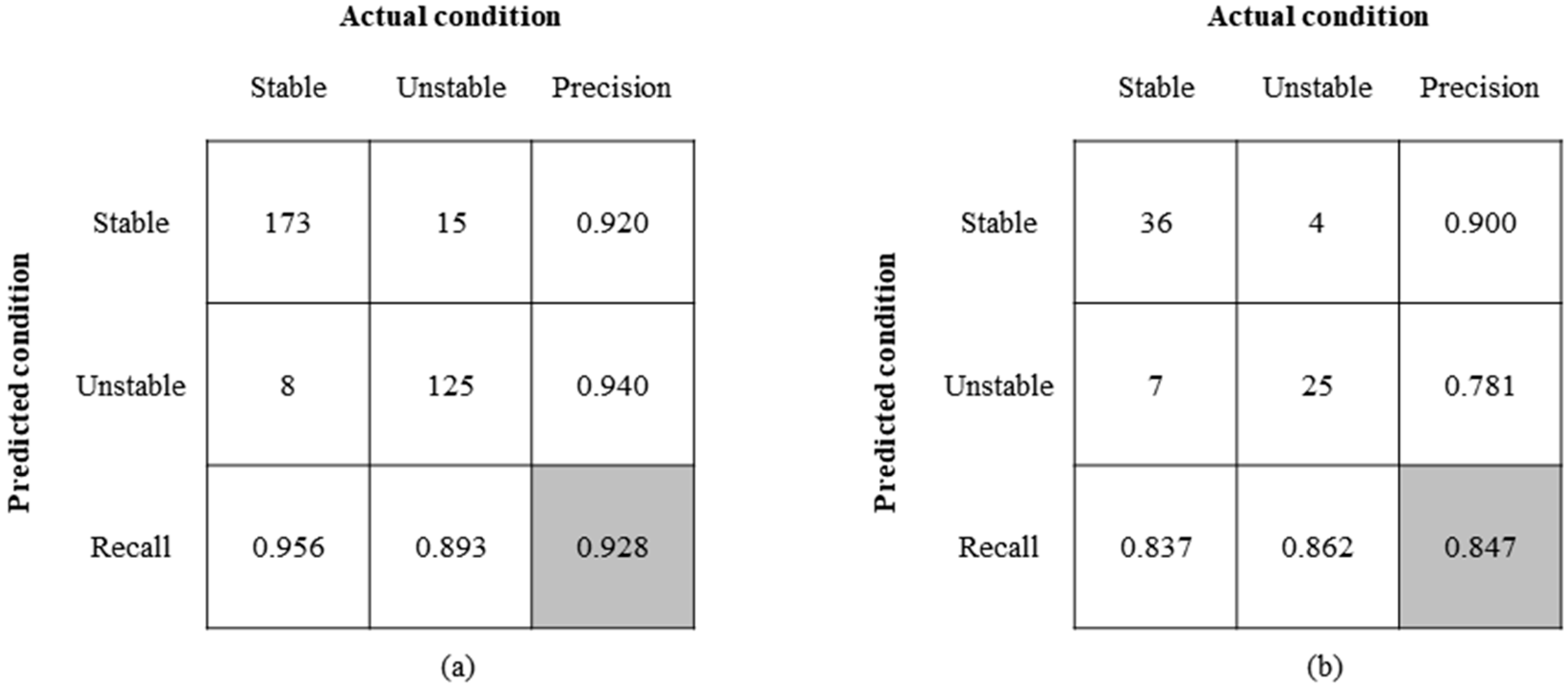
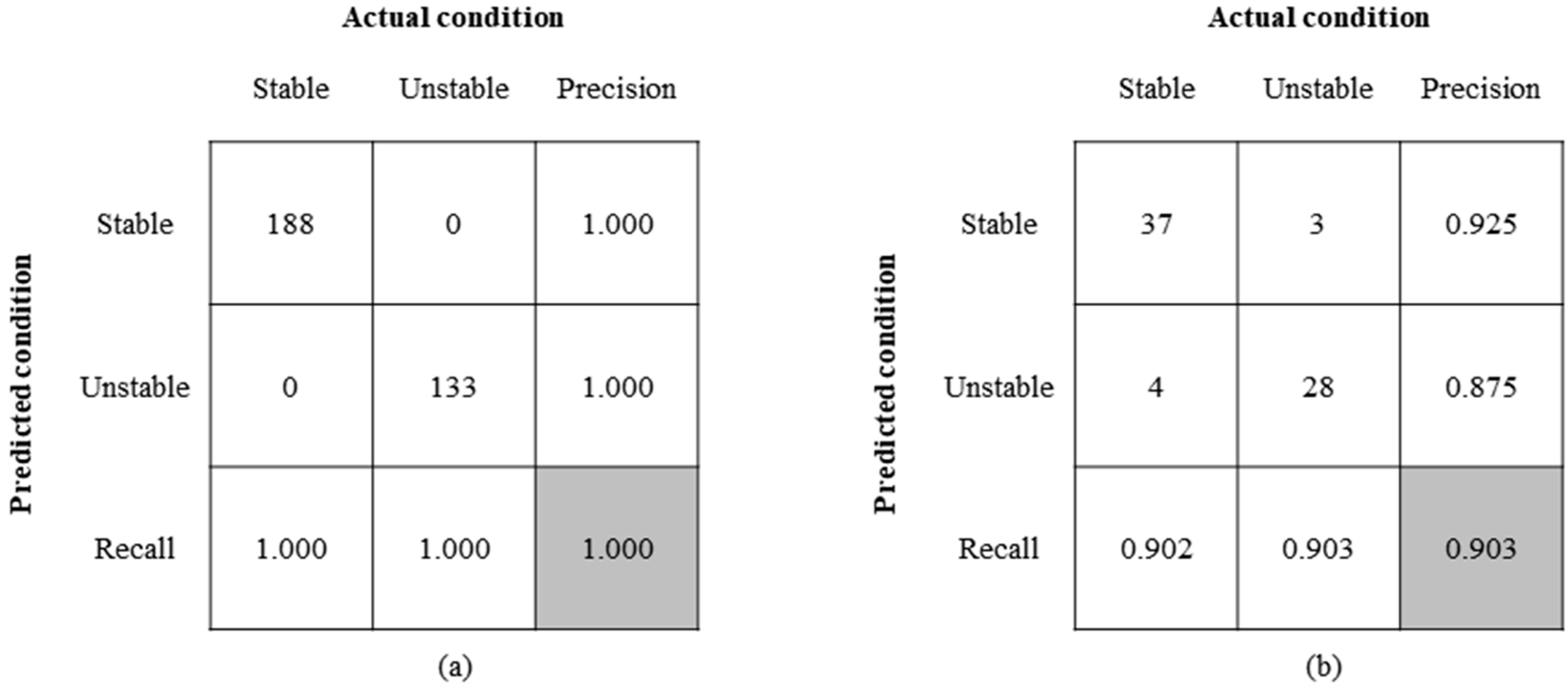
3. Results
3.1. Predictive Performance of Different Machine Learning Models
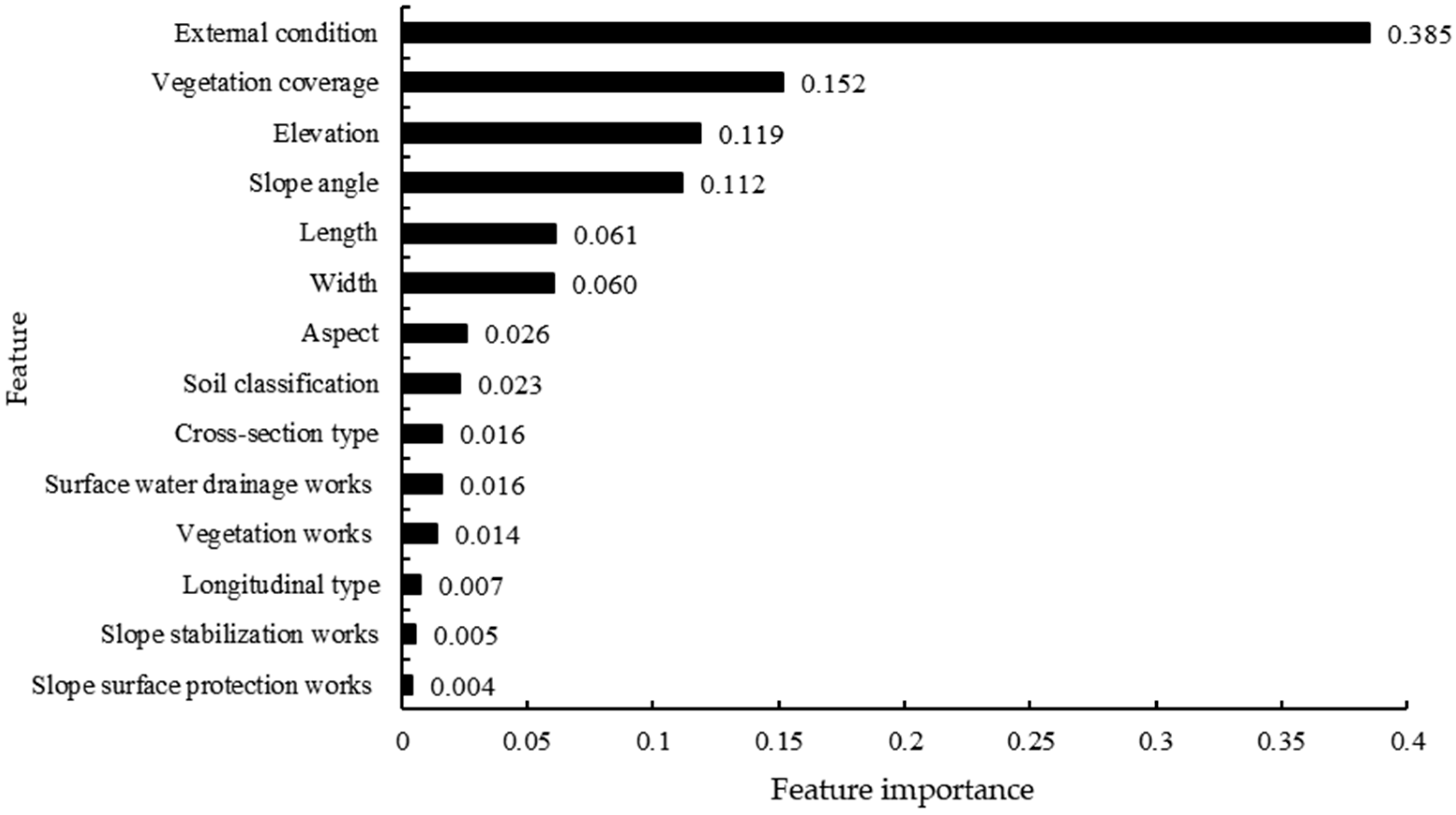
3.2. Feature Importance Analysis
4. Discussion
5. Conclusions
Author Contributions
Funding
Data Availability Statement
Acknowledgments
Conflicts of Interest
References
- Shin, H.T.; Yi, M.H.; Lee, C.H.; Sung, J.W.; Kim, K.S.; Kwon, Y.H.; Kim, S.J.; An, J.B.; Heo, T.I.; Yoon, J.W. The flora of vascular plants in the construction site of the National DMZ Native Botanic Garden. Korean J. Plant Resour. 2014, 27, 293–308. [Google Scholar] [CrossRef] [Green Version]
- Heo, T.I.; Shin, H.T.; Kim, S.J.; Lee, J.W.; Jung, S.Y.; An, J.B. The flora of Gwangchiryeong area adjacent to the DMZ. Korean J. Environ. Ecol. 2017, 31, 1–23. [Google Scholar] [CrossRef]
- An, J.B.; Shin, H.T.; Jung, S.Y.; Yoon, J.W.; Heo, T.I.; Lee, J.W.; Kim, S.J. The flora of Mt. Daedeukbong (Cheorwon-gun, Gangwon-do) in DMZ area of Korea. Korean J. Environ. Ecol. 2018, 32, 355–372. [Google Scholar] [CrossRef]
- Kim, S.J.; Shin, H.T.; An, J.B.; Yoon, J.W.; Jung, S.Y.; Lee, J.W.; Heo, T.I. The floristic study of Mt. Bonghwa (yanggu-gun, gangwon-do) area adjacent to the korean demilitarized zone. Korean J. Plant Resour. 2018, 31, 554–574. [Google Scholar]
- NamGung, J.; Yoon, C.Y.; Ha, Y.H.; Kim, J.H. The flora of Mt. Papyeong (Gyeonggi-do Prov.) in western area of DMZ, Korea. Korean J. Plant Resour. 2019, 32, 355–378. [Google Scholar]
- Song, J.H.; Byun, K.R.; Gil, H.Y. Vascular plant diversity of Sambong and Jaung Mountains in Paju City, border area of the Korean DMZ. Korean J. Environ. Ecol. 2022, 36, 30–55. [Google Scholar] [CrossRef]
- Yun, H.G.; Lee, J.W.; Jung, S.Y.; Hwang, H.S.; Bak, G.P.; Park, J.S.; Kim, S.J. Distribution Characteristic of Vascular Plants in Mt. Masan at Goseong-gun, Gangwon-do, Korea. Korean J. Plant Resour. 2022, 35, 71–99. [Google Scholar]
- Gantsetseg, A.; Jung, S.Y.; Cho, W.B.; Han, E.K.; So, S.K.; Lee, J.H. Definition and species list of northern lineage plants on the Korean Peninsula. Korean Herb. Med. Inform. 2020, 8, 183–204. [Google Scholar]
- Kim, O.S.; Václavík, T.; Park, M.S.; Neubert, M. Understanding the Intensity of Land-Use and Land-Cover Changes in the Context of Postcolonial and Socialist Transformation in Kaesong, North Korea. Land 2022, 11, 357. [Google Scholar] [CrossRef]
- Lee, J.W.; An, J.B.; Kang, S.H.; Yun, H.G. A study on the flora of outstanding forest wetlands in the eastern part of Jeonnam Province. Korean J. Plant Res. 2022, 35, 134–167. [Google Scholar]
- NA, H.S.; PARK, J.M.; LEE, J.S. Analysis of land cover classification and pattern using remote sensing and spatial statistical method-Focusing on the DMZ region in Gangwon-Do. J. Korean Assoc. Geogr. Inf. Stud. 2015, 18, 100–118. [Google Scholar] [CrossRef]
- KWON, S.; KIM, E.; LIM, J.; YANG, A.R. The Analysis of Changes in Forest Status and Deforestation of North Korea’s DMZ Using RapidEye Satellite Imagery and Google Earth. J. Korean Assoc. Geogr. Inf. Stud. 2021, 24, 113–126. [Google Scholar]
- Monitoring of Mountainous Areas within CACZ and Formulation of Management Plans for Damaged Forest Lands; Korean Forest Service: Daejeon, Republic of Korea, 2020.
- Devkota, K.C.; Regmi, A.D.; Pourghasemi, H.R.; Yoshida, K.; Pradhan, B.; Ryu, I.C.; Dhital, M.R.; Althuwaynee, O.F. Landslide susceptibility mapping using certainty factor, index of entropy and logistic regression models in GIS and their comparison at Mugling–Narayanghat road section in Nepal Himalaya. Nat. Hazards 2013, 65, 135–165. [Google Scholar] [CrossRef]
- Qi, C.; Tang, X. Slope stability prediction using integrated metaheuristic and machine learning approaches: A comparative study. Comput. Ind. Eng. 2018, 118, 112–122. [Google Scholar] [CrossRef]
- Kardani, N.; Zhou, A.; Nazem, M.; Shen, S.L. Improved prediction of slope stability using a hybrid stacking ensemble method based on finite element analysis and field data. J. Rock Mech. Geotech. Eng. 2021, 13, 188–201. [Google Scholar] [CrossRef]
- Sun, D.; Wen, H.; Zhang, Y.; Xue, M. An optimal sample selection-based logistic regression model of slope physical resistance against rainfall-induced landslide. Nat. Hazards 2021, 105, 1255–1279. [Google Scholar] [CrossRef]
- Kadavi, P.R.; Lee, C.W.; Lee, S. Landslide-susceptibility mapping in Gangwon-do, South Korea, using logistic regression and decision tree models. Environ. Earth Sci. 2019, 78. [Google Scholar] [CrossRef]
- Zhang, T.; Han, L.; Han, J.; Li, X.; Zhang, H.; Wang, H. Assessment of landslide susceptibility using integrated ensemble fractal dimension with kernel logistic regression model. Entropy 2019, 21, 218. [Google Scholar] [CrossRef] [Green Version]
- Sujatha, E.R.; Sridhar, V. Landslide susceptibility analysis: A logistic regression model case study in Coonoor, India. Hydrology 2021, 8, 41. [Google Scholar] [CrossRef]
- Jiang, J.; Kamel, M.S. Aggregation of reinforcement learning algorithms. In Proceedings of the 2006 IEEE International Joint Conference on Neural Network Proceedings, Vancouver, BC, Canada, 16–21 July 2006. [Google Scholar]
- Akgun, A. A comparison of landslide susceptibility maps produced by logistic regression, multi-criteria decision, and likelihood ratio methods: A case study at İzmir, Turkey. Landslides 2012, 9, 93–106. [Google Scholar] [CrossRef]
- Asteris, G.; Rizal, F.I.M.; Koopialipoor, M.; Roussis, P.C.; Ferentinou, M.; Armaghani, D.J.; Gordan, B. Slope stability classification under seismic conditions using several tree-based intelligent techniques. Appl. Sci. 2022, 12, 1753. [Google Scholar] [CrossRef]
- Taalab, K.; Cheng, T.; Zhang, Y. Mapping landslide susceptibility and types using Random Forest. Big Earth Data 2018, 2, 159–178. [Google Scholar] [CrossRef]
- Sun, D.; Wen, H.; Wang, D.; Xu, J. A random forest model of landslide susceptibility mapping based on hyperparameter optimization using Bayes algorithm. Geomorphology 2020, 362, 107201. [Google Scholar] [CrossRef]
- Lee, S.; Hong, S.M.; Jung, H.S. A support vector machine for landslide susceptibility mapping in Gangwon Province, Korea. Sustainability 2017, 9, 48. [Google Scholar] [CrossRef] [Green Version]
- Moayedi, H.; Tien Bui, D.; Kalantar, B.; Kok Foong, L. Machine-learning-based classification approaches toward recognizing slope stability failure. Appl. Sci. 2019, 9, 4638. [Google Scholar] [CrossRef] [Green Version]
- Niu, P.F.; Zhou, A.H.; Huang, H.C. Assessing model of highway slope stability based on optimized SVM. China Geol. 2020, 3, 339–344. [Google Scholar] [CrossRef]
- Zhang, W.; Li, H.; Han, L.; Chen, L.; Wang, L. Slope stability prediction using ensemble learning techniques: A case study in Yunyang County, Chongqing, China. J. Rock Mech. Geotech. Eng. 2022, 14, 1089–1099. [Google Scholar] [CrossRef]
- Xu, W.; Kang, Y.; Chen, L.; Wang, L.; Qin, C.; Zhang, L.; Liang, D.; Wu, C.; Zhang, W. Dynamic assessment of slope stability based on multi-source monitoring data and ensemble learning approaches: A case study of Jiuxianping landslide. Geol. J. 2022, 58, 2353–2371. [Google Scholar] [CrossRef]
- Bharti, J.P.; Mishra, P.; Sathishkumar, V.E.; Cho, Y.; Samui, P. Slope stability analysis using Rf, gbm, cart, bt and xgboost. Geotech. Geol. Eng. 2021, 39, 3741–3752. [Google Scholar] [CrossRef]
- Mulyono, A.; Subardja, A.; Ekasari, I.; Lailati, M.; Sudirja, R.; Ningrum, W. The hydromechanics of vegetation for slope stabilization. In Proceedings of the IOP Conference Series: Earth and Environmental Science, Bandung, Indonesia, 18–19 October 2018; p. 012038. [Google Scholar]
- Hou, S.; Liu, Y.; Yang, Q. Real-time prediction of rock mass classification based on TBM operation big data and stacking technique of ensemble learning. J. Rock Mech. Geotech. Eng. 2022, 14, 123–143. [Google Scholar] [CrossRef]
- Breiman, L. Random forests. Mach. Learn. 2001, 45, 5–32. [Google Scholar] [CrossRef] [Green Version]
- Chen, W.; Zhang, S.; Li, R.; Shahabi, H. Performance evaluation of the GIS-based data mining techniques of best-first decision tree, random forest, and naïve Bayes tree for landslide susceptibility modeling. Sci. Total Environ. 2018, 644, 1006–1018. [Google Scholar] [CrossRef] [PubMed]
- Khalilia, M.; Chakraborty, S.; Popescu, M. Predicting disease risks from highly imbalanced data using random forest. BMC Med. Inform. Decis. Mak. 2011, 11, 51. [Google Scholar] [CrossRef] [Green Version]
- Boser, B.E.; Guyon, I.M.; Vapnik, V.N. A training algorithm for optimal margin classifiers. In Proceedings of the Fifth Annual Workshop on Computational Learning Theory, Pittsburgh, PA, USA, 27–29 July 1992. [Google Scholar]
- Kavzoglu, T.; Sahin, E.K.; Colkesen, I. Landslide susceptibility mapping using GIS-based multi-criteria decision analysis, support vector machines, and logistic regression. Landslides 2014, 11, 425–439. [Google Scholar] [CrossRef]
- Mountrakis, G.; Im, J.; Ogole, C. Support vector machines in remote sensing: A review. ISPRS J. Photogramm. Remote Sens. 2011, 66, 247–259. [Google Scholar] [CrossRef]
- Friedman, J.H. Greedy function approximation: A gradient boosting machine. Ann. Stat. 2001, 29, 1189–1232. [Google Scholar] [CrossRef]
- Ming, L. Machine Learning; Tsinghua University Press: Beijing, China, 2019; pp. 187–189. [Google Scholar]
- Cox, D.R. The regression analysis of binary sequences. J. R. Stat. Soc. Ser. B (Methodol.) 1958, 20, 215–232. [Google Scholar] [CrossRef]
- Li, Y.; Li, M.; Li, C.; Liu, Z. Forest aboveground biomass estimation using Landsat 8 and Sentinel-1A data with machine learning algorithms. Sci. Rep. 2020, 10, 9952. [Google Scholar] [CrossRef]
- Bissuel, A. Hyper-Parameter Optimization Algorithms: A Short Review. Medium (Blog), 16 April 2019. Available online: https://medium.com/criteo-engineering/hyper-parameter-optimization-algorithms-2fe447525903 (accessed on 3 June 2023).
- Powers, D.M. Evaluation: From Precision, Recall and f-Factor to Roc, Informedness, Markedness and Correlation; Technical Report SIE-07-001; School of Informatics and Engineering, Flinders University of South Australia: Adelaide, Australia, 2007. [Google Scholar]
- Bradley, A.P. The use of the area under the ROC curve in the evaluation of machine learning algorithms. Pattern Recognit. 1997, 30, 1145–1159. [Google Scholar] [CrossRef] [Green Version]
- Saldanha, G.; O’Brien, S. Research Methodologies in Translation Studies; Routledge: New York, NY, USA, 2014; pp. 154–196. [Google Scholar]
- Landis, J.R.; Koch, G.G. The measurement of observer agreement for categorical data. Biometrics 1977, 33, 159–174. [Google Scholar] [CrossRef] [PubMed] [Green Version]
- Zhang, W.; Wu, C.; Zhong, H.; Li, Y.; Wang, L. Prediction of undrained shear strength using extreme gradient boosting and random forest based on Bayesian optimization. Geosci. Front. 2021, 12, 469–477. [Google Scholar] [CrossRef]
- Shetty, S.S.; Hoang, D.C.; Gupta, M.; Panda, S.K. Learning desk fan usage preferences for personalised thermal comfort in shared offices using tree-based methods. Build. Environ. 2019, 149, 546–560. [Google Scholar] [CrossRef]
- Lu, P.; Liu, H.; Serratella, C.; Wang, X. Assessment of data-driven, machine learning techniques for machinery prognostics of offshore assets. In Proceedings of the Offshore Technology Conference, Houston, TX, USA, 1–4 May 2017. [Google Scholar]
- Act No. 19077; The Military Base and Facilities Protection Act (MBFPA). Ministry of National Defense: Seoul, Republic of Korea, 2022.
- Yang, Y.; Zhou, W.; Jiskani, I.M.; Lu, X.; Wang, Z.; Luan, B. Slope Stability Prediction Method Based on Intelligent Optimization and Machine Learning Algorithms. Sustainability 2023, 15, 1169. [Google Scholar] [CrossRef]
- Bischetti, G.B.; Chiaradia, E.A.; D’agostino, V.; Simonato, T. Quantifying the effect of brush layering on slope stability. Ecol. Eng. 2010, 36, 258–264. [Google Scholar] [CrossRef]
- Guyon, I.; Gunn, S.; Nikravesh, M.; Zadeh, L.A. Feature Extraction: Foundations and Applications; Springer: Berlin/Heidelberg, Germany, 2005. [Google Scholar]
- Lin, Y.; Zhou, K.; Li, J. Prediction of slope stability using four supervised learning methods. IEEE Access 2018, 6, 31169–31179. [Google Scholar] [CrossRef]
- Wang, G.; Zhao, B.; Wu, B.; Zhang, C.; Liu, W. Intelligent prediction of slope stability based on visual exploratory data analysis of 77 in situ cases. Int. J. Min. Sci. Technol. 2023, 33, 47–59. [Google Scholar] [CrossRef]
- Pandian, S. K-Fold Cross Validation Technique and Its Essentials. Analytics Vidhya (Blog), 24 August 2022. Available online: https://www.analyticsvidhya.com/blog/2022/02/k-fold-cross-validation-technique-and-its-essentials/ (accessed on 3 June 2023).
- Koopialipoor, M.; Jahed Armaghani, D.; Hedayat, A.; Marto, A.; Gordan, B. Applying various hybrid intelligent systems to evaluate and predict slope stability under static and dynamic conditions. Soft Comput. 2019, 23, 5913–5929. [Google Scholar] [CrossRef]
- Luo, Z.; Bui, X.N.; Nguyen, H.; Moayedi, H. A novel artificial intelligence technique for analyzing slope stability using PSO-CA model. Eng. Comput. 2021, 37, 533–544. [Google Scholar] [CrossRef]
- Pham, K.; Kim, D.; Park, S.; Choi, H. Ensemble learning-based classification models for slope stability analysis. Catena 2021, 196, 104886. [Google Scholar] [CrossRef]
- Lasserre, J.; Arnold, S.; Vingron, M.; Reinke, P.; Hinrichs, C. Predicting the outcome of renal transplantation. J. Am. Med. Inform. Assoc. 2012, 19, 255–262. [Google Scholar] [CrossRef] [Green Version]


| Classification | Feature | Type | Description |
|---|---|---|---|
| Slope conditions | Elevation | Number | Meter (m) |
| Slope angle | Number | Degree (°) | |
| Aspect | 4 categories | North, east, south, and west | |
| Soil classification | 8 categories | Clay loam (A), loamy (B), loamy and weathered rock (BD), sandy loam (C), sandy and weathered rock (CD), sandy loam and soft rock (CE), weathered rock (D), and soft rock (E) | |
| Cross-sectional type | 4 categories | Convex, parallel, concave, and combined | |
| Longitudinal type | 4 categories | Convex, parallel, concave, and combined | |
| Vegetation conditions | Vegetation works | 2 categories | Presence and absence |
| Vegetation coverage | 3 categories | Good, moderate, and poor | |
| Structure conditions | Width of the structure | Number | Meter (m) |
| Length of the structure | Number | Meter (m) | |
| Slope stabilization works | 2 categories | Presence and absence | |
| Slope surface protection works | 2 categories | Presence and absence | |
| Surface water drainage works | 2 categories | Presence and absence | |
| External condition | 3 categories | Good, moderate, and poor |
| Grade | Training Data | Test Data | Total |
|---|---|---|---|
| Stable | 188 (0.586) | 40 (0.556) | 228 (0.580) |
| Unstable | 133 (0.414) | 32 (0.444) | 165 (0.420) |
| Sum | 321 | 72 | 393 |
| Predicted Class | Actual Class | |
|---|---|---|
| Positive | Negative | |
| Positive | True positive (TP) | False positive (FP) |
| Negative | False negative (FN) | True negative (TN) |
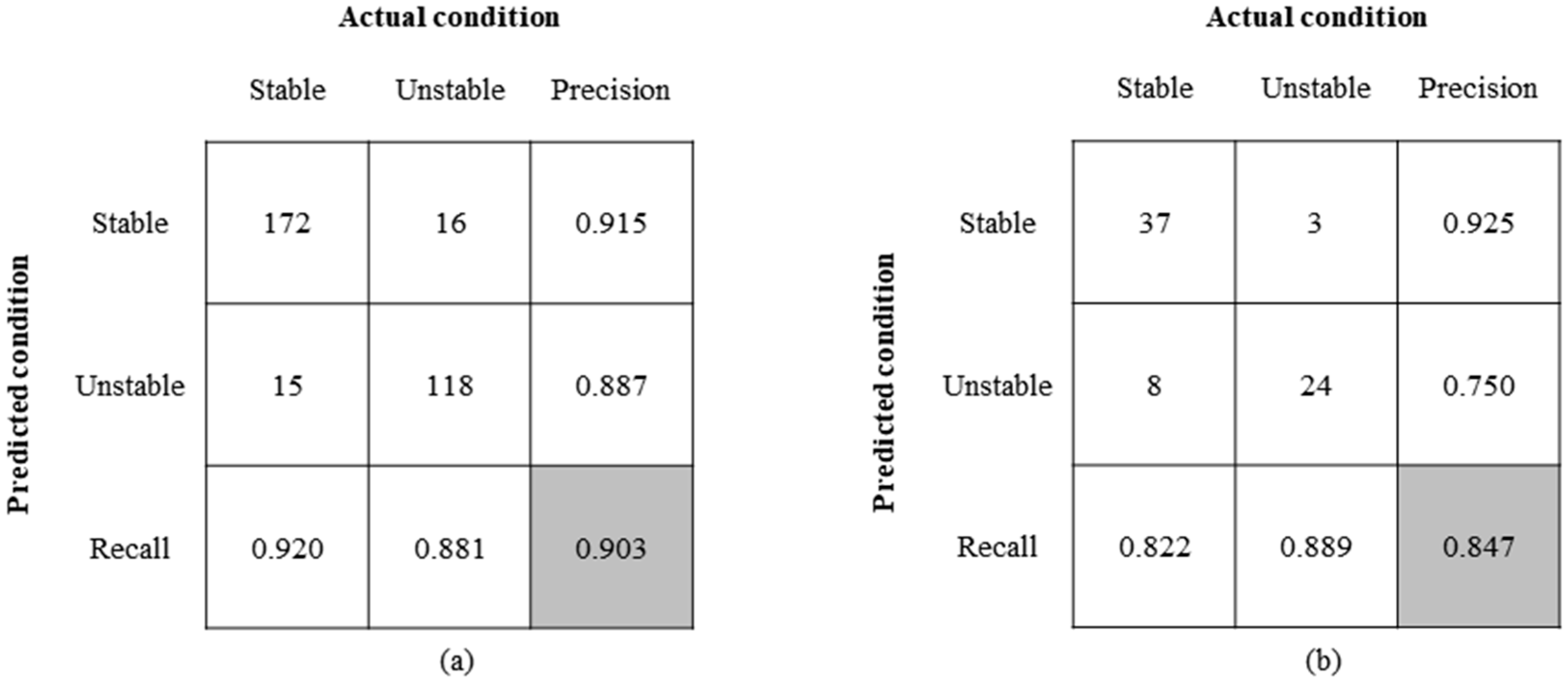
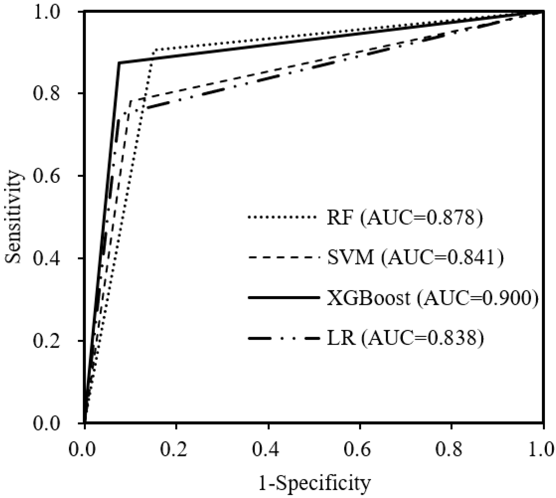
| ML Algorithm | F1-Score | Kappa Value | Recall Rate | Precision |
|---|---|---|---|---|
| RF | 0.883 | 0.749 | 0.850 | 0.919 |
| SVM | 0.867 | 0.688 | 0.837 | 0.900 |
| XGBoost | 0.914 | 0.803 | 0.902 | 0.925 |
| LR | 0.871 | 0.686 | 0.822 | 0.925 |
Disclaimer/Publisher’s Note: The statements, opinions and data contained in all publications are solely those of the individual author(s) and contributor(s) and not of MDPI and/or the editor(s). MDPI and/or the editor(s) disclaim responsibility for any injury to people or property resulting from any ideas, methods, instructions or products referred to in the content. |
© 2023 by the authors. Licensee MDPI, Basel, Switzerland. This article is an open access article distributed under the terms and conditions of the Creative Commons Attribution (CC BY) license (https://creativecommons.org/licenses/by/4.0/).
Share and Cite
Kwon, S.; Pan, L.; Kim, Y.; Lee, S.I.; Kweon, H.; Lee, K.; Yeom, K.; Seo, J.I. Empirical Comparison of Supervised Learning Methods for Assessing the Stability of Slopes Adjacent to Military Operation Roads. Forests 2023, 14, 1237. https://doi.org/10.3390/f14061237
Kwon S, Pan L, Kim Y, Lee SI, Kweon H, Lee K, Yeom K, Seo JI. Empirical Comparison of Supervised Learning Methods for Assessing the Stability of Slopes Adjacent to Military Operation Roads. Forests. 2023; 14(6):1237. https://doi.org/10.3390/f14061237
Chicago/Turabian StyleKwon, SeMyung, Leilei Pan, Yongrae Kim, Sang In Lee, Hyeongkeun Kweon, Kyeongcheol Lee, Kyujin Yeom, and Jung Il Seo. 2023. "Empirical Comparison of Supervised Learning Methods for Assessing the Stability of Slopes Adjacent to Military Operation Roads" Forests 14, no. 6: 1237. https://doi.org/10.3390/f14061237