Article

Zoning Prediction and Mapping of Three-Dimensional Forest Soil Organic Carbon: A Case Study of Subtropical Forests in Southern China

1
Guangdong Academy of Forestry, 233 Guangshan First Road, Tianhe District, Guangzhou 510520, China
2
Faculty of Forestry, University of British Columbia, Vancouver, BC V6T 1Z4, Canada
3
Guangxi Institute of Botany, Guangxi Zhuang Autonomous Region and Chinese Academy of Sciences, Guilin 541006, China
*
Author to whom correspondence should be addressed.
Forests 2023, 14(6), 1197; https://doi.org/10.3390/f14061197
Submission received: 19 April 2023 / Revised: 28 May 2023 / Accepted: 6 June 2023 / Published: 9 June 2023
(This article belongs to the Special Issue Soil Carbon, Nitrogen and Phosphorus Changes in Forests)

Abstract

:
Accurate soil organic carbon (SOC) maps are helpful for guiding forestry production and management. Different ecological landscape areas within a large region may have different soil–landscape relationships, so models specifically for these areas may capture these relationships more accurately than the global model for the entire study area. The aim of this study was to investigate the role of zonal modelling in predicting forest SOC and to produce highly accurate forest SOC distribution maps. The prediction objects were SOC at five soil depths (0–20, 20–40, 40–60, 60–80, and 80–100 cm). First, the forest type map and soil texture class map were used to divide the relative homogeneous regions in Shaoguan City, Guangdong Province, China. Second, seven terrain variables derived from a 12.5-m digital elevation model (DEM) and five vegetation variables generated from 10-m Sentinel-2 remote sensing images were used as predictors to develop regional artificial neural network (ANN) models for each homogeneous region, as well as a global ANN model for the entire study area (1000 sample points). Finally, 10-fold cross-validation was used to assess the ANN prediction model performance, and independent validation was used to evaluate the produced forest SOC prediction maps (194 additional samples). The cross-validation results showed that the accuracies of the regional models were better than that of the global model. Independent validation results also showed that the precision (R2) of 0- to 100-cm forest SOC maps generated by forest type modelling had an improvement of 0.05–0.15, and that by soil texture class modelling had an improvement of 0.07–0.13 compared to the map generated by the global model. In conclusion, delineating relatively homogeneous regions via simple methods can improve prediction accuracy when undertaking soil predictions over large areas, especially with complex forest landscapes. In addition, SOC in the study area is generally more abundant in broadleaf forest and clay areas, with overall levels decreasing with soil depth. Accurate SOC distribution information can provide references for fertilization and planting. Plants with particularly high soil fertility requirements may perhaps be planted in broadleaf forests or clay areas, and plants with particularly developed roots may require furrow application of a small amount of SOC.

1. Introduction

Forest ecosystems store about 70%–80% of terrestrial carbon, which is an important global carbon sink, as approximately half of all carbon is accumulated in mineral forest soil [1]. Adequate organic carbon content can enhance the water retention capacity of forest soil and improve soil structure and permeability, which are conducive to improving plant growth and protecting forest resources [2,3]. Therefore, the study of soil organic carbon (SOC) content, distribution, and variation can lead to a better understanding of the carbon cycle process of forest ecosystems and provide important references and support for forest resource protection, ecosystem management, and global climate change research [4].
Efficient techniques should be used to precisely measure variations in forest SOC within fields, which is important for field management. Based on Jenny’s [5] and Huggett’s [6] theoretical foundations, various models have been established to predict the spatial distribution of soil properties according to the relationships between target soil characteristics and environmental covariates [7,8]. The artificial neural network (ANN) model is well known for its efficient processing of a large amounts of data from different sources (with different noise levels and accuracies) and good generalizability [9]. Chagas et al. [10] and Taghizadeh-Mehrjardi et al. [11] showed that an ANN had the best performance when predicting SOC compared to other data mining techniques. In forest soil modelling, ANN models have become a popular tool in recent years.
Different geographical regions in a large range of areas may have different soil–landscape relationships, but many forest soil mapping efforts adopt a single model to achieve the prediction for the whole region [12]. It is difficult for only one model to completely construct multiple distinctive soil-environment relationships at the same time. Consequently, modelling specifically for these regions may more accurately capture these relationships [13]. Song et al. [14] argued that global modelling that considers all regions simultaneously may fail to simulate SOC at specific points, which may lead to unreasonable spatial predictions. If a region contains two or more different patterns of spatial variation, it seems wise to model these regions independently to maximize the use of the method [15]. Thus, dividing relatively homogeneous geographical units seems to be a promising prospect.
Similar soil-forming conditions develop similar soil properties [16]. Based on this assumption, a complex forest area can be divided into several relatively homogeneous units with less heterogeneity. Recently, the impact of regional segmentation on soil prediction maps has been recognized [15]. For example, Mulder et al. [17] and Ross et al. [13] both found that the spatial variation of an SOC map based on zoning modelling obtained higher prediction accuracy. Sun et al. [18] identified that the accuracy of models varied significantly between different geomorphic types. Peng et al. [19] divided a study region into upland and wetland areas. Most existing studies segment areas by topographic features and land types but ignore that basic soil data can provide valuable information for digital soil mapping (DSM). According to McBratney et al. [20], basic soil information can be used in DSM. Soil conservation capacity, nutrient cycle, pH, and biodiversity will be different under different vegetation types [21]. Soil texture has an impact on soil permeability, water retention capacity, and nutrient holding capacity [22]. The qualitative soil–landscape relationships of these data (forest class vector maps and texture maps) can be used as prior knowledge of soil variation, which may help to generate realistic soil maps conforming to soil formation conditions [23]. This basic information is usually used as covariates of models [17] but not as methods to segment regions. Therefore, this study was based on the information provided by the basic soil data for zoning, building a separate model for each region. In addition, almost all soil assessment studies that have applied zonal modelling approaches have only explored the soil surface layer and have not considered deeper soils. However, a large number of soil nutrients are also stored at deeper layers [23], and detailed and accurate information about deeper soils is scarce.
Moreover, simply mosaicking the region predictions can lead to boundary artifacts and discontinuous patterns [24]. This phenomenon is due to the method of dividing homogeneous zones, which leads to abrupt changes in the boundaries of different landscapes [25]. The apparent division between landscapes leads to a discontinuous distribution of SOC in space, which may result in some unreasonable predictions [26]. Therefore, it is more appropriate to use an ensemble approach to produce the SOC distribution pattern maps at a locale. The utility of ensemble modelling has been demonstrated by McBratney et al. [27] and Taghizadeh-Mehrjardi [11]. The usual research evaluates multiple models and then selects the best performing model. However, each model has its own strengths and weaknesses in any particular case. Integrating multiple training models is an alternative that helps to combine the knowledge and information obtained from different models, resulting in greater accuracy of prediction and classification [28].
To maximize the accuracy of forest SOC reasoning and reduce the interference of multiple factors, this study reconstructed the complex surface space under the guidance of a geographical analysis. This study aimed to improve the predictive ability of ANN models for SOC via zoning modelling. At the same time, the purpose was to provide high-precision SOC distribution maps for forest management. The main objectives of this study were to: (1) segment the study area into several relatively independent soil prediction regions based on forest type maps and soil texture maps; (2) develop the global ANN model based on the entire study area and regional ANN models based on each subregion for the 0- to 100-cm forest SOC; and (3) compare these two modelling methods and use an ensemble approach to produce the study area forest SOC map.

2. Materials and Methods

2.1. Study Area and Soil Data

Covering an area of 18,400 km2, Shaoguan City (23°53′–25°31′ N, 112°53′–114°45′ E) is the second largest city in Guangdong Province, China (Figure 1). With 74.46% forest coverage, Shaoguan is a key forest area in China and the base of the timber forests and bamboo fields in Guangdong. The mean annual temperature is approximately 21 °C, the average annual rainfall is about 1700 mm, the summers are hot and humid, and the winters are warm and dry [29]. The topography mainly consists of mountains and hills, with higher elevations in the north and lower elevations in the south. The stratigraphic development is basically complete, but the various rock types are scattered. The rock types are mainly glutenite, sandstone, metamorphic rock, granite, and limestone. The soil texture in the study area mainly consists of clay, clay loam, loam, and sandy loam. Overall, the forest type and soil texture class in Shaoguan are representative, which is an important reference value for zoning modelling.
Soil profiles (n = 1194) were collected by the 2020 Forest Soil Survey Project of the Guangdong Academy of Forestry Sciences (Figure 1). The sampling points were set by combining a thematic distribution with a spatial random distribution to ensure that all environmental gradient changes and major forest types were covered. A 1-m-deep soil pit was dug at each sampling site. If the profile had no record before the 1-m depth, the soil profile was excavated down to the parent material horizon. The soil was sampled at fixed depth increments of 0–20, 20–40, 40–60, 60–80, and 80–100 cm. At each depth, no less than 500 g of soil was collected and taken back to the laboratory, where it was air dried, ground, sieved (2 mm), and stored in glass bottles for chemical analysis. SOC was determined by the potassium dichromate oxidation external heating method [30].

2.2. Environmental Variables

2.2.1. Model Covariates

The 12 covariates that mainly represent soil formation were derived from the 12.5-m digital elevation model (DEM) and the 10-m Sentinel-2 satellite images (Table 1). The DEM image used in this study was obtained from the NASA Earth Science Data website (https://nasadaacs.eos.nasa.gov/ (accessed on 15 June 2019)) and was resampled to 10-m raster using ArcGIS v10.7.1 software of Environmental Systems Research Institute (Redlands, CA, USA). Seven topographical variables—slope, aspect, topographical position index (TPI), topographic wetness index (TWI), flow accumulation (FA), soil terrain factor (STF), and stream power index (SPI)—were derived from the resampled DEM. Terrain affects the movement of water, including the transportation and deposition of sediment, so the size of these terrain variables represents the soil retention capacity [31,32,33].
The clearest multispectral remote sensing image covering the study area came from eight Level-1C cloudless images from Sentinel-2 on the Copernicus data-sharing website of the European Space Agency (https://scihub.copernicus.eu/ (accessed on 20 September 2021)). Then, we used the SNAP v9.0.0 software of European Space Agency (Paris, France) Sen2cor plug-in provided by the European Space Agency to perform atmospheric correction on the original Level-1C image, thus obtaining L2A image data. Moreover, the images were resampled to 10-m resolution and converted into the ENVI format for export. In ENVI v5.6.3 software of Exelis Visual Information Solutions (Boulder, CO, USA), all bands except 2, 3, 4, and 8 were removed, and only these four bands were retained to generate images. This paper also used the mathematical function of ENVI v5.6.3 to extract five vegetation indices: normalized difference vegetation index (NDVI), differential vegetation index (DVI), ratio vegetation index (RVI), reformed difference vegetation index (RDVI), and enhanced vegetation index (EVI). These combinations (vegetation indices) are simple and effective indicators to detect vegetation growth status and vegetation coverage, and they can also eliminate some radiation errors [34,35].

2.2.2. Zoning Method

Two methods were used for region segmentation (Figure 2). First, the study area was segmented into broad-leaved forest, coniferous forest, and mixed coniferous and broad-leaved forests according to the forest type vector map provided by the National Forestry and Grassland Science Data Center of China (http://www.forestdata.cn/ (accessed on 6 March 2019)). Second, based on the 250-m T_USDA_TEX (0–30 cm) and S_USDA_TEX (30–100 cm) maps provided by the World Soil Database (https://www.fao.org/home/en/ (accessed on 15 February 2023)), the upper soil texture (0–40 cm) of the study area was segmented into clay and sandy loam, and the deep soil texture (40–100 cm) was classified as clay and clay loam.

2.3. Prediction Technique

2.3.1. ANN Model Structure and Training

ANNs can easily and accurately establish complex nonlinear relationships between independent and dependent variables, as well as manage incomplete, noisy, and ambiguous data without extensive data processing. An ANN consists of the input layer, hidden layer, and output layer, and the basic units of the network are nodes (also called neurons), equivalent to biological neurons. The nodes in the input layer disperse all the prediction variables to each node in the hidden layer. Then, the hidden layer nodes realize the nonlinear transformation of information through the activation function (Sigmoid). Finally, the output layer nodes accept the output results of the hidden layer and calculate the errors. The ANN updates the network by back-transferring the errors. The process of information traversing from the input layer to the output layer (forward propagation) and from the output layer to the input layer (back propagation) is a training loop.
Ten-fold cross-validation was implemented to train the model. The training set was used to calculate the gradient and update the network weight and deviation, and the validation set was used to stop the network operation in advance. The error of the training set decreased with increasing iterations, and the verification error also decreased gradually at the beginning of training. However, if the network started to overfit, the error on the verification set began to increase. Therefore, the early stop technique was used to avoid network overfitting by stopping training when the training error decreased, but the independent verification error increased.

2.3.2. Screening Model

Including all covariates in the model may increase the uncertainty of the model [36]. For this study, the covariates were entered into the model in combinations of 1 to 12 variables ( C 12 1 ,   C 12 2 ,   C 12 3 ,   C 12 4 ,   C 12 5 ,   C 12 6 ,   C 12 7 ,   C 12 8 ,   C 12 9 ,   C 12 10 ,   C 12 11   and   C 12 12 ). There were 4095 combinations of 12 variables, corresponding to 4095 ANN models. The optimal model was selected based on the accuracy indices after 10-fold cross-validation of the 4095 ANN models.

2.4. Mapping Method

To solve the problem of discontinuity in the prediction map due to the simple mosaic, this study referred to the methods used by Song et al. [14] and Brungard et al. [37] and utilized ensemble learning to produce the final predicted SOC maps of the entire area. The specific calculation is as follows:
f f i n a l = k 1   f f + k 2   f t + k 3   f g
where f f and f t are the zoning predictions maps by forest type and soil texture class, respectively; f g is the prediction map for the global model (entire study area); and k1, k2, and k3 are the coefficients of the three modelling methods. The values of k 1 , k 2 and k 3 were set by comparing the performances of the three models (Table 2). This research specified that one model significantly outperformed the others when the difference between the R2 values of the two models was >5%.

2.5. Accuracy Metrics

Two validation methods were used to evaluate the ANN model: 10-fold cross-validation of the global and regional models and independent validation of the forest SOC maps generated by the different methods based on the extra 194 samples. Three precision indices were used for the validation. Root mean square error (RMSE) is a measure of the model’s prediction error. R2 is a measure of the goodness of fit of the model. Relative overall accuracy (ROA) is a metric for the prediction accuracy of the model [38]. The specific formulas were as follows:
R M S E = i = 1 n Y i X i 2 n
R 2 = i = 1 n ( X i Y i ) 2 i = 1 n ( X i   Y i ¯ ) 2
R O A = i = 1 n 1   if   abs Y i   X i X i   ×   100   <   T 0   else n ×   100
where Y I is the predicted value, I is the measured value, n is number of samples, I i ¯ is the mean of the model predictions, and T is the accuracy threshold (e.g., 10 for 10% in this study), determined based on the target to fit the model.

2.6. Statistical Analysis

The ANN predictive method was implemented with Matlab v9.7 of MathWorks (Natick, MA, USA). R v4.1.1 of R Core Team (Vienna, Austria) was used for statistical analysis. In detail, the normality of the SOC data for the five soil layers was determined according to the Shapiro–Wilk test at ≥0.9, and if it was not satisfied, log transformation was performed. Differences in SOC among three forest types were tested by ANOVA with Duncan’s multiple comparison test. The difference in SOC between the two texture classes was tested using the t-test. Soil mapping was performed with ArcGIS software, version 10.7.

3. Results

3.1. Exploratory Data Analysis

A visual representation of the sample zoning shows that each homogeneous region had a different sample size (Figure 3a), but the sampling densities were similar (0.08–0.09 km2). The average level of forest SOC showed a general decreasing trend in variation from 0 to 100 cm (Figure 3b). There were significant differences in forest SOC between the soil layers except for those at 60–80 cm and 80–100 cm. SOC content varied from 0.09 to 93.13 g kg−1. For the zoning method according to forest type, the SOC of different forest types was significantly different except at depths of 60–80 cm and 80–100 cm (Table S1). For the zoning measure of soil texture type, the SOC of each soil texture class was significantly different. This finding implies that the pedogenetic characteristics of these homogeneous zones were significantly different.

3.2. Descriptive Statistics of Prediction Accuracy

3.2.1. Accuracies of Global Models

This study first constructed the global ANN model (Table 3). Generally, adding more effective variables can gradually improve the accuracy of the model, but this improvement will not be sustained when the increased parameters exceed a certain number. When the seventh variable was added to the 0- to 20-cm ANN model, the RMSE value became larger, and the R2 and ROA became smaller. This outcome was not surprising because the accumulated error of the input variable itself would increase the uncertainty of the model to a certain extent, and this degree of uncertainty would lead to the deterioration of the model accuracy if it exceeded the improvement in the model accuracy. Consequently, the optimal model could be determined when increasing the number of variables in the model did not significantly improve the accuracy results.

3.2.2. Accuracies of Zone Modelling

The same screening method as above—screening the ANN model with as small as possible a value for RMSE and as large as possible values of R2 and ROA—was adopted to screen the optimal model. The optimal model accuracies of 0- to 100-cm SOC for different forest types in the study area showed RMSEs ranging from 13.99 to 50.51 g kg−1, R2 from 0.75 to 0.90, and ROAs from 65.44% to 82.41% (Table 4). The optimal model accuracy for 0- to 100-cm SOC of different soil texture classes indicated RMSEs ranging from 17.08 to 48.93 g kg−1, R2 from 0.71 to 0.82, and ROAs from 65.14% to 73.31% (Table 5). The model accuracies (RMSE, R2, and ROA) of the homogeneous regions were almost always greater than those of the global model (Table 3 vs. Table 4 and Table 5).
The 12 covariates all appeared in the optimal model, indicating that each of the selected terrain and vegetation variables were valid predictors. However, the optimal combinations of variables were different for different soil layers, and it may be that the drivers of dynamic local variation are different for different soil depths. Aspect and slope had the highest frequencies in the optimal combination of model variables, indicating that aspect and slope had greater influences on the spatial distribution of SOC.

3.2.3. Accuracies of the Covariate Models

To further demonstrate the necessity of zoning modelling, the categories for forest types and soil texture classes were entered into the global models as covariates (Table 6). The covariate combinations of some optimal models did not contain corresponding covariates. Furthermore, the accuracies of the models containing the corresponding covariates were not significantly improved compared to those of the original global models. For example, the ANN model containing the forest type covariate with the largest increase in R2 value was only 0.05 in the 0- to 20-cm soil layer.

3.2.4. Independent Verification

Both the regional and covariate models outperformed the global model in terms of accuracy after 10-fold cross-validation. However, we could not yet draw any conclusions because whether this outcome was the result of model overfitting due to the reduced sample size or the role of zoning was unknown. Therefore, further judgment was needed through independent validation (Figure 4). The covariate model seemed to have the highest RMSE and the lowest R2 and ROA, indicating that the results of the 10-fold cross-validation may be a case of overfitting. The independent validation accuracies of the regional models were higher rather than lower than those of the global models, indicating that the zonal approach improved the accuracy of the prediction maps, and this improvement overcame the overfitting due to the reduced sample size. Overall, the independent validation accuracy of both zoning methods deteriorated with soil depth. The R2 values for zoning by forest type were 0.61–0.78, representing an improvement of 0.05–0.15 compared to the global model, while the R2 values for zoning by soil texture class were 0.63–0.76, representing an improvement of 0.07–0.13 compared to the global model.

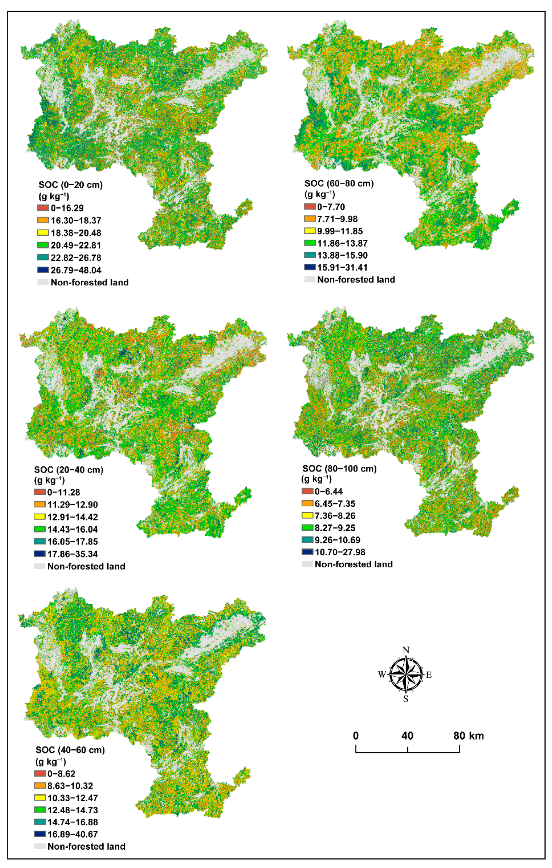
3.3. Digital Forest SOC Maps

In this study, different types of ANN models were used to predict and map SOC, some of which showed insignificant differences in performance. Ensemble learning is able to combine the advantages of each model and shows better performance than a single type of model. The ensemble coefficients of each soil layer are shown in Table S2. The independent validation accuracies (R2) of the five soil depth maps (Figure 5) produced by ensemble learning were 0.78, 0.74, 0.68, 0.65, and 0.66, respectively, which were slightly higher than the independent validation accuracies of the single model shown in Figure 4. The forest SOC prediction maps produced by the ensemble approach did not show significant discontinuities. The average forest SOC contents of the five soil layers in the study area were 21.17, 13.87, 12.43, 11.23, and 9.29 g kg−1, and the forest SOC content decreased with soil depth. The distribution pattern of SOC at 0–20 cm mainly showed a low content in the middle and high content in the surrounding area. The low value areas of 20–40 cm SOC were scattered throughout the study area, and the high value areas were mainly distributed in the eastern broadleaf forest localities. The low value areas of 40–60, 60–80, and 80–100 cm SOC were distributed throughout the study area, but the high value areas of 40–60 cm SOC were mainly distributed in the north, and the high value areas of 60–80 and 80–100 cm SOC were mainly distributed in the south. Overall, SOC was more abundant in broadleaf forests and clay areas. Referring to the classification standard of soil organic matter in the second soil survey of China, 1.724 was used as the conversion coefficient between SOC and organic matter [39]. In this study, the forest SOC in Shaoguan City was classified into six classes: very lacking (0–3.48 g kg−1), lacking (3.48–5.80 g kg−1), medium (5.80–11.60 g kg−1), rich (11.60–17.40 g kg−1), very rich (17.40–23.20 g kg−1), and extremely rich (>23.20 g kg−1) (Figure 6). The overall forest SOC of 0–40 cm was generally greater than the rich class, indicating that the vegetation with underdeveloped root systems of Shaoguan forest land was little constrained by SOC. Starting from the layer of 40–60 cm, SOC gradually transitioned to medium class with soil depth. The overall forest SOC at 80–100 cm was medium class.

4. Discussion

4.1. Performance of Zoning Modelling

This study focused on comparing global models, zonal models (two types) and covariate models (two types). Independent validation results showed that zonal modelling obtained the best predictive performance compared to both the global model and covariate models (forest type and soil texture were used as covariates). Compared with the global model, the accuracies (R2) of predicting 0- to 100-cm SOC by forest type was improved by 0.05–0.15, and that by soil texture classes was improved by 0.07–0.13. This outcome was due to the large variation in soil-forming characteristics in the study area; global modelling can only simulate the main characteristics of these complex correlations, which are not sufficient to simulate soil variations in different soil zones [14]. The prediction by zoning approach can suppress some of the interference of the complex soil–environment relationship.
The results of the multiple comparisons (see Table S1) also showed significant differences in SOC among different forest types and different soil texture classes in the study area, suggesting that SOC should be assessed separately for each area. In Belgium, Lettens et al. [40] divided their study area into 289 landscape units and predicted the SOC in each landscape unit. In France, Mulder et al. [17] segmented their study area into 10 soil landscape types and modelled regressions between SOC and environmental variables for each landscape. They found that categorical predictions at each soil landscape unit could better explain SOC heterogeneity. Uniform predictions of fields do not consider spatial variability, which is often not the most effective mapping strategy [41]. The accuracy of zoning modelling in this study was better than the accuracy of entering the zoning methods into the model as covariates. This finding further illustrates that it is necessary to explicitly model by each region rather than rely on covariates to capture the variability between regions. This conclusion is consistent with [37], who found that the accuracy of the global model did not change significantly when the zonal strategies were input as covariates.
It is worth noting that, after segmenting the area, the sample of each homogeneous area will be reduced relative to the global model, which can easily lead to overfitting. Lai et al. [42] and Sun et al. [18] also recognized that the sample size affects the accuracy of the model. Therefore, the 10-fold cross-validation method is not rigorous enough to judge whether the zoning method can improve the prediction; it needs to be further analyzed by combining those results with the independent validation results. If the improvement in model accuracy was entirely due to overfitting, then the regional model would possess poor generalizability, and the independent validation of the regional model would be lower than that of the global model [43]. Conversely, the higher independent validation proves that zonal modelling can indeed help the model to better simulate the SOC variation pattern. In fact, this improvement should be larger than the number obtained from the study because this improvement is the result of offsetting the negative effects of overfitting due to the reduced sample size. Thus, the actual R2 maximum predicted increase obtained by the zoning method in this study was larger than 0.15. Many studies of zonal models have focused on topsoil (0–30 cm). The maximum improvement in precision (R2) of our zonal model was smaller (0.07) than that of Wang et al. [24], probably because our validation sample points were 31 times more numerous than theirs. In addition, the present study obtained slightly higher zoning accuracy than other studies [14,18,44]. However, mapping accuracy varies with different landscape types, modelling methods, and sample sizes. Therefore, the findings in the literature regarding methods that perform better in a given domain cannot be generalized [18].
In addition, this study showed that there were differences in the predictive ability of the regional model at each SOC depth. The predicted ability of zoning by forest type and soil texture class decreased with soil depth. This finding may account for the inconsistent effectiveness of stands, texture, and soil-forming rocks at different soil depths. Ziche et al. [21] also concluded that vegetation has a greater impact on the upper soil layer and that the impact of vegetation on the soil is mainly influenced by its apoplast and roots, while deeper soils have less vegetation apoplast and roots. Jobbágy and Jackson [45] found that the effect of soil texture on SOC increased with increasing soil depth. The reason that this study did not yield better improvements in deeper soils may be that the differences in the effects of the two textures on SOC were not sufficiently pronounced, with no pronounced differences between the two soil textures (clay and clay loam) in the study area at 40–100 cm according to the US soil texture classification criteria [46], and more pronounced differences between the two soil textures (clay and sandy loam) at 0–40 cm. Therefore, more significant differences between homogeneous zones result in better zonal modelling results.

4.2. Predicted Distribution of Forest SOC Content

In supervised learning algorithms for machine learning, the goal is to train a stable model that performs well in all aspects. In practice, this goal is often not possible, and instead multiple models with better performance in some aspects are obtained [28]. However, an over-performing model may have overfitting problems, while multiple preferred models combined into one model are not prone to overfitting problems. Different but related competing models can be combined into one result that is at least as good as any individual result [47]. Ensemble learning may lead to better and more stable predictions. Case studies of soil mapping have typically used the best results based on model comparisons [44,48,49]. In contrast, we used ensemble learning to integrate predictions from a single ANN model. Our SOC maps were better than those from other regional SOC prediction studies [50,51,52,53,54].
The combined use of vegetation and topographic variables effectively tapped into the spatial variability of the soil. The spatial content of SOC in the study area gradually decreased with soil depth. Song et al. [14] and Zhang et al. [55] also found lower SOC content in deeper soil. Decomposing matter is generally concentrated in surface forest soils, and the high temperatures and precipitation encourage bacterial activity. These conditions increase the decomposition of organic matter, leading to the enrichment of forest soil SOC in the upper soil [21]. In terms of horizontal structure, the areas with higher SOC content were generally broadleaf forest areas with flatter terrain. This result arose from the combination of topography and tree species characteristics. Higher concentrations of complex secondary compounds, such as lignin and tannins, slow the decomposition rate so that decomposition occurs faster in broadleaf forests and slower in coniferous forests [56]. The higher degree of slope leads to higher rates of erosion, which increases with increasing rainfall. Hence, high slopes have a greater SOC loss because of the less developed soil profile and relatively thin soil layer [57,58]. In addition, aspect is also important for the spatial variation in the SOC. Sunny slopes generally have lower SOC content than shady slopes. Hydrological and solar conditions vary with aspect, leading to differences in vegetation composition and distribution patterns, in turn affecting SOC decomposition rates [59]. Clay particles can effectively increase SOC accumulation by hindering SOM decomposition, slowing the SOC renewal rate, and reducing SOC leaching through adsorption and aggregation [60,61]. Therefore, higher SOC content is usually found in the clay zone.
In short, due to the different spatial distributions of forest SOC content, both fertilization patterns and planting patterns should consider the local SOC content. In broadleaf forests and clay areas, it may be more appropriate to grow plants with higher soil fertility requirements due to higher SOC content. Fertilization patterns should also be different for plants with inconsistent root systems [62,63]. Plants with root systems mainly in the 0- to 40-cm soil layer do not need to be considered for SOC application, plants with root systems in the 40- to 80-cm range may need to be considered for a small amount of SOC furrow application in localized areas, and plants with root systems mainly below 80 cm need to be considered for a small amount of SOC furrow application in the entire study area. Therefore, it is important to know the three-dimensional variation in forest SOC to improve the fertilization efficiency and forest productivity.

4.3. Limitations

Although this study achieved better forest SOC content predictions based on the segmented region approach and ensemble learning, there are still some limitations. First, there may have been sampling and experimental errors in the data collection and laboratory analysis. Second, the method of segmenting homogeneous areas is based on vegetation type maps and soil texture maps, and the resolution of these qualitative maps was coarser than the target resolution (10 m), so the homogeneous areas segmented by this method may not be homogeneous enough. Therefore, it would be better to include quantitative environmental information in the segmentation process in the future. Third, some uncertainties in the prediction covariates were inevitably involved in the prediction process. For example, errors arose from the extraction of topographic variables from digital elevation models and vegetation variables from remotely sensed images. These uncertainties were indirectly propagated to the SOC content prediction maps. Finally, only the ANN model with the three-layer structure was used to explore the effect of partition modelling in this study. Deep-learning neural networks with multiple hidden layers and improved training algorithms or other soil models could also be considered in future soil mapping work.

5. Conclusions

In this study, two zonal modelling approaches and ensemble learning were used to predict the three-dimensional spatial distribution of depth-specific SOC over a large forest area. The forest type map and soil texture class map were utilized to divide the modelling area, resulting in several relatively homogeneous regions being modelled separately. This paper also compared the regional models with the global model (entire study area) and the covariate model (forest type and soil texture class as covariates), and the independent validation showed that the regional model had the best accuracy, while the covariate model had the worst generalization performance. The utility of regional modelling by forest type and soil texture class decreased with soil depth. The R2 for the regional model by forest type ranged from 0.61 to 0.78, which was an improvement of 0.05–0.15 compared to the global model, while the R2 values for the regional model by soil texture class varied from 0.63 to 0.76, which was an improvement of 0.07–0.13 compared to the global model. This outcome demonstrates that segmenting areas based on easily accessible soil information, such as forest type and soil texture, can efficiently improve the predictive power of the forest soil prediction model. In conclusion, the present study found zonal modelling to be promising for forest soil mapping and recommends further investigation of zonal modelling to extrapolate to larger areas.

Supplementary Materials

The following supporting information can be downloaded at: https://www.mdpi.com/article/10.3390/f14061197/s1, Table S1: The results of Duncan’s multiple comparison test and t-tests for SOC (g kg−1) in homogeneous regions; Table S2: The ensemble coefficients of each soil layer.

Author Contributions

Conceptualization, Y.L., Z.Z. (Zhengyong Zhao) and X.D.; methodology, Y.L., Z.Z. (Zhengyong Zhao), D.S. and X.D.; software, Y.L. and X.Z.; validation, X.D.; formal analysis, Y.L. and X.Z.; investigation, Z.Z. (Zhongrui Zhang), D.S., H.Z. and G.Z.; resources, X.D. and Z.Z. (Zhongrui Zhang); data curation, Z.Z. (Zhongrui Zhang); writing—original draft preparation, Y.L.; writing—review and editing, X.D.; visualization, Y.L. and X.Z.; supervision, X.D.; project administration, X.D. and Z.Z. (Zhongrui Zhang); funding acquisition, X.D. All authors have read and agreed to the published version of the manuscript.

Funding

This work was funded by Forestry Administration of Guangdong Province (grant nos. 2023KJCX021 and 2022KJQT004).

Data Availability Statement

Not applicable.

Acknowledgments

Not applicable.

Conflicts of Interest

The authors declare no conflict of interest.

References

  1. Nitsch, P.; Kaupenjohann, M.; Wulf, M. Forest continuity, soil depth and tree species are important parameters for SOC stocks in an old forest (Templiner Buchheide, northeast Germany). Geoderma 2018, 310, 65–76. [Google Scholar] [CrossRef]
  2. Qiu, T.; Andrus, R.; Aravena, M.-C.; Ascoli, D.; Bergeron, Y.; Berretti, R.; Berveiller, D.; Bogdziewicz, M.; Boivin, T.; Bonal, R.; et al. Limits to reproduction and seed size-number trade-offs that shape forest dominance and future recovery. Nat. Commun. 2022, 13, 1238. [Google Scholar] [CrossRef] [PubMed]
  3. Mayer, M.; Rusch, S.; Didion, M.; Baltensweiler, A.; Walthert, L.; Ranft, F.; Rigling, A.; Zimmermann, S.; Hagedorn, F. Elevation dependent response of soil organic carbon stocks to forest windthrow. Sci. Total Environ. 2023, 857, 159694. [Google Scholar] [CrossRef] [PubMed]
  4. Jandl, R.; Rodeghiero, M.; Martinez, C.; Cotrufo, M.F.; Bampa, F.; van Wesemael, B.; Harrison, R.B.; Guerrini, I.A.; Richter, D.D.; Rustad, L.; et al. Current status, uncertainty and future needs in soil organic carbon monitoring. Sci. Total Environ. 2014, 468–469, 376–383. [Google Scholar] [CrossRef]
  5. Jenny, H. Factors of Soil Formation. Soil Sci. 1941, 52, 415. [Google Scholar] [CrossRef]
  6. Huggett, R.J. Soil landscape systems: A model of soil Genesis. Geoderma 1975, 13, 1–22. [Google Scholar] [CrossRef]
  7. Minasny, B.; McBratney, A. Digital soil mapping: A brief history and some lessons. Geoderma 2016, 264, 301–311. [Google Scholar] [CrossRef]
  8. Scull, P.; Franklin, J.; Chadwick, O.A.; McArthur, D. Predictive soil mapping: A review. Prog. Phys. Geogr. Earth Environ. 2003, 27, 171–197. [Google Scholar] [CrossRef] [Green Version]
  9. Chen, L.; Ren, C.; Li, L.; Wang, Y.; Zhang, B.; Wang, Z.; Li, L. A Comparative Assessment of Geostatistical, Machine Learning, and Hybrid Approaches for Mapping Topsoil Organic Carbon Content. ISPRS Int. J. Geo-Inf. 2019, 8, 174. [Google Scholar] [CrossRef] [Green Version]
  10. Chagas, C.D.S.; Vieira, C.A.O.; Filho, E.I.F. Comparison between artificial neural networks and maximum likelihood classification in digital soil mapping. Rev. Bras. Ciênc. Solo 2013, 37, 339–351. [Google Scholar] [CrossRef]
  11. Taghizadeh-Mehrjardi, R.; Nabiollahi, K.; Kerry, R. Digital mapping of soil organic carbon at multiple depths using different data mining techniques in Baneh region, Iran. Geoderma 2016, 266, 98–110. [Google Scholar] [CrossRef]
  12. Guevara, M.; Olmedo, G.F.; Stell, E.; Yigini, Y.; Aguilar Duarte, Y.; Arellano Hernández, C.; Arévalo, G.E.; Arroyo-Cruz, C.E.; Bolivar, A.; Bunning, S.; et al. No Silver Bullet for Digital Soil Mapping: Country-Specific Soil Organic Carbon Estimates across Latin America. Soil Methods 2018, 4, 173–193. [Google Scholar] [CrossRef] [Green Version]
  13. Ross, C.W.; Grunwald, S.; Vogel, J.G.; Markewitz, D.; Jokela, E.J.; Martin, T.A.; Bracho, R.; Bacon, A.R.; Brungard, C.W.; Xiong, X. Accounting for two-billion tons of stabilized soil carbon. Sci. Total Environ. 2020, 703, 134615. [Google Scholar] [CrossRef]
  14. Song, X.-D.; Wu, H.-Y.; Ju, B.; Liu, F.; Yang, F.; Li, D.-C.; Zhao, Y.-G.; Yang, J.-L.; Zhang, G.-L. Pedoclimatic zone-based three-dimensional soil organic carbon mapping in China. Geoderma 2020, 363, 114145. [Google Scholar] [CrossRef]
  15. McBratney, A.B.; Hart, G.A.; McGarry, D. The use of region partitioning to improve the representation of geo statistically mapped soil attributes. J. Soil Sci. 1991, 42, 513–532. [Google Scholar] [CrossRef]
  16. Hudson, B.D. The Soil Survey as Paradigm-based Science. Soil Sci. Soc. Am. J. 1992, 56, 836–841. [Google Scholar] [CrossRef]
  17. Mulder, V.L.; Lacoste, M.; Richer-De-Forges, A.C.; Martin, M.P.; Arrouays, D. National versus global modelling the 3D distribution of soil organic carbon in mainland France. Geoderma 2016, 263, 16–34. [Google Scholar] [CrossRef]
  18. Sun, X.-L.; Lai, Y.-Q.; Ding, X.; Wu, Y.-J.; Wang, H.-L.; Wu, C. Variability of soil mapping accuracy with sample sizes, modelling methods and landform types in a regional case study. Catena 2022, 213, 106217. [Google Scholar] [CrossRef]
  19. Peng, Y.; Xiong, X.; Adhikari, K.; Knadel, M.; Grunwald, S.; Greve, M.H. Modeling Soil Organic Carbon at Regional Scale by Combining Multi-Spectral Images with Laboratory Spectra. PLoS ONE 2015, 10, e0142295. [Google Scholar] [CrossRef] [Green Version]
  20. McBratney, A.B.; Mendonça Santos, M.L.; Minasny, B. On digital soil mapping. Geoderma 2003, 117, 3–52. [Google Scholar] [CrossRef]
  21. Ziche, D.; Grüneberg, E.; Hilbrig, L.; Höhle, J.; Kompa, T.; Liski, J.; Repo, A.; Wellbrock, N. Comparing soil inventory with modelling: Carbon balance in central European forest soils varies among forest types. Sci. Total. Environ. 2019, 647, 1573–1585. [Google Scholar] [CrossRef] [PubMed]
  22. Poggio, L.; Gimona, A. 3D mapping of soil texture in Scotland. Geoderma Reg. 2017, 9, 5–16. [Google Scholar] [CrossRef]
  23. Meersmans, J.; van Wesemael, B.; De Ridder, F.; Van Molle, M. Modelling the three-dimensional spatial distribution of soil organic carbon (SOC) at the regional scale (Flanders, Belgium). Geoderma 2009, 152, 43–52. [Google Scholar] [CrossRef]
  24. Wang, S.; Adhikari, K.; Zhuang, Q.; Yang, Z.; Jin, X.; Wang, Q.; Bian, Z. An improved similarity-based approach to predicting and mapping soil organic carbon and soil total nitrogen in a coastal region of northeastern China. PeerJ 2020, 8, e9126. [Google Scholar] [CrossRef] [PubMed]
  25. Jaeger, J.A.G. Landscape division, splitting index, and effective mesh size: New measures of landscape fragmentation. Landsc. Ecol. 2000, 15, 115–130. [Google Scholar] [CrossRef]
  26. Rosenbloom, N.A.; Harden, J.W.; Neff, J.C.; Schimel, D.S. Geomorphic control of landscape carbon accumulation. J. Geophys. Res. 2006, 111, G01004. [Google Scholar] [CrossRef]
  27. Malone, B.P.; Minasny, B.; Odgers, N.P.; McBratney, A.B. Using model averaging to combine soil property rasters from legacy soil maps and from point data. Geoderma 2014, 232–234, 34–44. [Google Scholar] [CrossRef]
  28. Swiderski, B.; Osowski, S.; Kruk, M.; Barhoumi, W. Aggregation of classifiers ensemble using local discriminatory power and quantiles. Expert Syst. Appl. 2016, 46, 316–323. [Google Scholar] [CrossRef]
  29. Li, T.; Li, M.; Ren, F.; Tian, L. Estimation and Spatio-Temporal Change Analysis of NPP in Subtropical Forests: A Case Study of Shaoguan, Guangdong, China. Remote Sens. 2022, 14, 2541. [Google Scholar] [CrossRef]
  30. Nóbrega, G.N.; Ferreira, T.O.; Artur, A.G.; de Mendonça, E.S.; de O. Leão, R.A.; Teixeira, A.S.; Otero, X.L. Evaluation of methods for quantifying organic carbon in mangrove soils from semi-arid region. J. Soils Sediments 2015, 15, 282–291. [Google Scholar] [CrossRef]
  31. Bangroo, S.A.; Najar, G.R.; Achin, E.; Truong, P.N. Application of predictor variables in spatial quantification of soil organic carbon and total nitrogen using regression kriging in the North Kashmir forest Himalayas. Catena 2020, 193, 104632. [Google Scholar] [CrossRef]
  32. Ding, X.; Zhao, Z.; Yang, Q.; Chen, L.; Tian, Q.; Li, X.; Meng, F.-R. Model prediction of depth-specific soil texture distributions with artificial neural network: A case study in Yunfu, a typical area of Udults Zone, South China. Comput. Electron. Agric. 2020, 169, 105217. [Google Scholar] [CrossRef]
  33. Zhao, Z.; Yang, Q.; Benoy, G.; Chow, T.L.; Xing, Z.; Rees, H.W.; Meng, F.-R. Using artificial neural network models to produce soil organic carbon content distribution maps across landscapes. Can. J. Soil Sci. 2010, 90, 75–87. [Google Scholar] [CrossRef]
  34. Mahmoudabadi, E.; Karimi, A.; Haghnia, G.H.; Sepehr, A. Digital soil mapping using remote sensing indices, terrain attributes, and vegetation features in the rangelands of northeastern Iran. Environ. Monit. Assess. 2017, 189, 500. [Google Scholar] [CrossRef]
  35. McGillem, C.D.; Svedlow, M. Short Papers Optimum Filter for Minimization of Image Registration Error Variance. IEEE Trans. Geosci. Electron. 1977, 15, 257–259. [Google Scholar] [CrossRef]
  36. Zhao, Z.; Yang, Q.; Sun, D.; Ding, X.; Meng, F.-R. Extended model prediction of high-resolution soil organic matter over a large area using limited number of field samples. Comput. Electron. Agric. 2020, 169, 105172. [Google Scholar] [CrossRef]
  37. Brungard, C.; Nauman, T.; Duniway, M.; Veblen, K.; Nehring, K.; White, D.; Salley, S.; Anchang, J. Regional ensemble modeling reduces uncertainty for digital soil mapping. Geoderma 2021, 397, 114998. [Google Scholar] [CrossRef]
  38. Zhao, Z.; Chow, T.L.; Rees, H.W.; Yang, Q.; Xing, Z.; Meng, F.-R. Predict soil texture distributions using an artificial neural network model. Comput. Electron. Agric. 2009, 65, 36–48. [Google Scholar] [CrossRef]
  39. Guangdong Soil Census Office. Guangdong Soil, 1st ed.; China Science Publishing: Beijing, China, 1993; p. 419. [Google Scholar]
  40. Lettens, S.; Van Orshoven, J.; Van Wesemael, B.; Muys, B. Soil organic and inorganic carbon contents of landscape units in Belgium derived using data from 1950 to 1970. Soil Use Manag. 2004, 20, 40–47. [Google Scholar] [CrossRef]
  41. Drăguţ, L.; Dornik, A. Land-surface segmentation as a method to create strata for spatial sampling and its potential for digital soil mapping. Int. J. Geogr. Inf. Sci. 2016, 30, 1359–1376. [Google Scholar] [CrossRef] [Green Version]
  42. Lai, Y.-Q.; Wang, H.-L.; Sun, X.-L. A comparison of importance of modelling method and sample size for mapping soil organic matter in Guangdong, China. Ecol. Indic. 2021, 126, 107618. [Google Scholar] [CrossRef]
  43. Fiorentini, N.; Pellegrini, D.; Losa, M. Overfitting Prevention in Accident Prediction Models: Bayesian Regularization of Artificial Neural Networks. Transp. Res. Rec. J. Transp. Res. Board 2023, 2677, 1455–1470. [Google Scholar] [CrossRef]
  44. Brungard, C.W.; Boettinger, J.L.; Duniway, M.C.; Wills, S.A.; Edwards, T.C. Machine learning for predicting soil classes in three semi-arid landscapes. Geoderma 2015, 239–240, 68–83. [Google Scholar] [CrossRef] [Green Version]
  45. Jobbágy, E.G.; Jackson, R.B. The vertical distribution of soil organic carbon and its relation to climate and vegetation. Ecol. Appl. 2000, 10, 423–436. [Google Scholar] [CrossRef]
  46. Fischer, G.F.; Nachtergaele, S.; Prieler, H.T.; van Velthuizen, L.; Verelst, D.W. Global Agro-Ecological Zones Assessment for Agriculture (GAEZ 2008); IIASA: Laxenburg, Austria; FAO: Rome, Italy, 2008. [Google Scholar]
  47. Wasson, T.; Hartemink, A.J. An ensemble model of competitive multi-factor binding of the genome. Genome Res. 2009, 19, 2101–2112. [Google Scholar] [CrossRef] [PubMed] [Green Version]
  48. Kumar, S.; Lal, R.; Liu, D. A geographically weighted regression kriging approach for mapping soil organic carbon stock. Geoderma 2012, 189–190, 627–634. [Google Scholar] [CrossRef]
  49. Song, X.-D.; Brus, D.J.; Liu, F.; Li, D.-C.; Zhao, Y.-G.; Yang, J.-L.; Zhang, G.-L. Mapping soil organic carbon content by geographically weighted regression: A case study in the Heihe River Basin, China. Geoderma 2016, 261, 11–22. [Google Scholar] [CrossRef]
  50. Bhunia, G.S.; Kumar Shit, P.; Pourghasemi, H.R. Soil organic carbon mapping using remote sensing techniques and multivariate regression model. Geocarto Int. 2019, 34, 215–226. [Google Scholar] [CrossRef]
  51. Rial, M.; Martinez Cortizas, A.; Taboada, T.; Rodríguez-Lado, L. Soil organic carbon stocks in Santa Cruz Island, Galapagos, under different climate change scenarios. Catena 2017, 156, 74–81. [Google Scholar] [CrossRef]
  52. Wang, K.; Zhang, C.; Li, W. Predictive mapping of soil total nitrogen at a regional scale: A comparison between geographically weighted regression and cokriging. Appl. Geogr. 2013, 42, 73–85. [Google Scholar] [CrossRef]
  53. Xu, Y.; Smith, S.E.; Grunwald, S.; Abd-Elrahman, A.; Wani, S.P.; Nair, V.D. Estimating soil total nitrogen in smallholder farm settings using remote sensing spectral indices and regression kriging. Catena 2018, 163, 111–122. [Google Scholar] [CrossRef] [Green Version]
  54. Yang, L.; Qi, F.; Zhu, A.-X.; Shi, J.; An, Y. Evaluation of Integrative Hierarchical Stepwise Sampling for Digital Soil Mapping. Soil Sci. Soc. Am. J. 2016, 80, 637–651. [Google Scholar] [CrossRef]
  55. Zhang, Z.; Zhou, Y.; Wang, S.; Huang, X. The soil organic carbon stock and its influencing factors in a mountainous karst basin in P. R. China. Carbonates Evaporites 2019, 34, 1031–1043. [Google Scholar] [CrossRef]
  56. Rasel, S.M.M.; Groen, T.A.; Hussin, Y.A.; Diti, I.J. Proxies for Soil Organic Carbon Derived from Remote Sensing. Int. J. Appl. Earth Obs. Geo-Inf. 2017, 59, 157–166. [Google Scholar] [CrossRef]
  57. Bookhagen, B.; Thiede, R.C.; Strecker, M.R. Abnormal monsoon years and their control on erosion and sediment flux in the high, arid northwest Himalaya. Earth Planet. Sci. Lett. 2005, 231, 131–146. [Google Scholar] [CrossRef]
  58. Mondal, A.; Khare, D.; Kundu, S.; Mondal, S.; Mukherjee, S.; Mukhopadhyay, A. Spatial soil organic carbon (SOC) prediction by regression kriging using remote sensing data. Egypt. J. Remote Sens. Space Sci. 2017, 20, 61–70. [Google Scholar] [CrossRef] [Green Version]
  59. Qin, Y.; Feng, Q.; Holden, N.M.; Cao, J. Variation in soil organic carbon by slope aspect in the middle of the Qilian Mountains in the upper Heihe River Basin, China. Catena 2016, 147, 308–314. [Google Scholar] [CrossRef]
  60. Burke, I.C.; Yonker, C.M.; Parton, W.J.; Cole, C.V.; Flach, K.; Schimel, D.S. Texture, Climate, and Cultivation Effects on Soil Organic Matter Content in U.S. Grassland Soils. Soil Sci. Soc. Am. J. 1989, 53, 800–805. [Google Scholar] [CrossRef]
  61. Wynn, J.G.; Bird, M.; Vellen, L.; Grand-Clement, E.; Carter, J.; Berry, S.L. Continental-scale measurement of the soil organic carbon pool with climatic, edaphic, and biotic controls: Continental-scale soil organic carbon. Glob. Biogeochem. Cycles 2006, 20. [Google Scholar] [CrossRef]
  62. Thomas, M.; Clifford, D.; Bartley, R.; Philip, S.; Brough, D.; Gregory, L.; Willis, R.; Glover, M. Putting regional digital soil mapping into practice in Tropical Northern Australia. Geoderma 2015, 241–242, 145–157. [Google Scholar] [CrossRef]
  63. Yang, Y.; Ouyang, S.; Gessler, A.; Wang, X.; Na, R.; He, H.S.; Wu, Z.; Li, M.-H. Root Carbon Resources Determine Survival and Growth of Young Trees under Long Drought in Combination with Fertilization. Front. Plant Sci. 2022, 13, 929855. [Google Scholar] [CrossRef] [PubMed]
Figure 1. Location, digital elevation model and sample points of Shaoguan City, Guangdong Province.
Forests 14 01197 g001
Figure 2. Maps of forest types and soil texture classes of Shaoguan City, Guangdong Province.
Forests 14 01197 g002
Figure 3. Statistical analysis of samples: (a) 1194 forest samples from 10 administrative districts of Shaoguan were classified according to forest type and soil texture class; (b) content of forest SOC in different soil layers; different lower-case letters denote significant differences (p < 0.05) after Duncan’s multiple comparison test.
Forests 14 01197 g003
Figure 4. Independent validation accuracies of each prediction method. Different colours denote different soil layers.
Forests 14 01197 g004
Figure 5. Forest SOC prediction maps for each soil layer produced by the ensemble approach.
Forests 14 01197 g005
Figure 6. Forest SOC prediction class maps for each soil layer.
Forests 14 01197 g006
Table 1. Covariates used for modelling SOC.
TypeCovariateAbbr.Resolution
DEM-derived terrain factorsSlopeSlope12.5 m
AspectAspect12.5 m
Topographic position indexTPI12.5 m
Topographic wetness indexTWI12.5 m
Flow accumulationFA12.5 m
Soil terrain factorSTF12.5 m
Stream power indexSPI12.5 m
Sentinel-2-derived vegetation factorsNormalized difference vegetation indexNDVI10 m
Differential vegetation indexDVI10 m
Ratio vegetation indexRVI10 m
Reformed difference vegetation indexRDVI10 m
Enhanced vegetation indexEVI10 m
Table 2. The candidate values of k1, k 2 and k 3 with ensemble learning.
K1K2K3Condition
100ff outperformed both ft and fg
010ft outperformed both ff and fg
001fg outperformed both ff and ft
1/21/20ff was similar to ft, and both ff and ft outperformed fg
1/201/2ff was similar to fg, and both ff and fg outperformed ft
01/21/2ft was similar to fg, and both ft and fg outperformed ff
1/31/31/3all three models were similar to each other
Table 3. Optimal variable combinations and 10-fold cross-validation accuracies of the global ANN model.
Layer (cm)Number aRMSE (g kg−1)R2ROA (%)Optimal Variable Combinations
0–20 C 12 1 131.810.2218.34Slope
C 12 2 111.890.3022.98Slope, NDVI
C 12 3 106.260.4736.25Slope, NDVI, SPI
C 12 4 88.410.5039.08Slope, NDVI, SPI, STF
C 12 5 75.360.5945.36Slope, NDVI, SPI, STF, Aspect
C 12 6 61.050.6556.52Slope, NDVI, SPI, STF, Aspect, EVI
C 12 7 66.560.6051.36Slope, NDVI, SPI, STF, Aspect, EVI, TWI
20–40 C 12 7 36.260.6861.16Aspect, Slope, STF, SPI, FA, DVI, NDVI
40–60 C 12 10 41.860.6654.81Slope, TWI, TPI, STF, SPI, FA, DVI, RDVI, NDVI, RVI
60–80 C 12 8 40.780.6456.13Aspect, Slope, STF, SPI, FA, EVI, DVI, NDVI
80–100 C 12 9 38.000.6557.87Aspect, Slope, TWI, TPI, STF, SPI, EVI, RDVI, RVI
Note: a The best combined variables were selected among all of combinations with the same number of variables based on the RMSE, R2, and ROA of the model. For example, the number of combinations with four variables is C 12 6 = 924. The abbreviations for the variables are defined in Table 1.
Table 4. Optimal variable combinations and 10-fold cross-validation accuracies of each zone divided by forest types.
Forest TypesLayer (cm)Number aRMSE (g kg−1)R2ROA (%)Optimal Variable Combinations
Broad-leaved0–20 C 12 9 50.510.8171.61Aspect, Slope, TWI, TPI, STF, SPI, DVI, RDVI, RVI
20–40 C 12 10 15.240.8674.35Aspect, Slope, TPI, STF, SPI, FA, EVI, RDVI, NDVI, RVI
40–60 C 12 9 23.510.8070.51Aspect, Slope, TPI, STF, SPI, FA, EVI, RDVI, RVI
60–80 C 12 9 23.460.7665.66Aspect, Slope, TWI, TPI, SPI, EVI, DVI, NDVI, RVI
80–100 C 12 5 22.740.7868.91Aspect, Slope, TPI, RDVI, RVI
Coniferous0–20 C 12 10 37.80.8375.75Aspect, Slope, TWI, TPI, STF, SPI, DVI, RDVI, NDVI, RVI
20–40 C 12 10 15.920.8071.08Aspect, Slope, TWI, TPI, STF, SPI, FA, EVI, NDVI, RVI
40–60 C 12 7 24.990.7666.55Aspect, TWI, TPI, STF, SPI, DVI, RDVI
60–80 C 12 7 21.260.7665.44Aspect, STF, SPI, EVI, DVI, RDVI, NDVI
80–100 C 12 9 23.830.7567.14Aspect, Slope, TWI, TPI, STF, SPI, FA, EVI, RVI
Mixed forest0–20 C 12 6 30.500.8777.15Slope, STF, EVI, DVI, NDVI, RVI
20–40 C 12 8 13.990.9082.41Aspect, Slope, TPI, STF, SPI, EVI, RDVI, NDVI
40–60 C 12 8 20.660.8472.01Aspect, TWI, TPI, STF, SPI, FA, EVI, RDVI
60–80 C 12 8 29.150.8069.12Aspect, Slope, TPI, SPI, EVI, DVI, RDVI, NDVI
80–100 C 12 7 16.070.8476.34Slope, TPI, SPI, FA, DVI, RDVI, RVI
Note: a same as Table 3. The abbreviations for the variables are defined in Table 1.
Table 5. Optimal variable combinations and 10-fold cross-validation accuracies of each zone divided by texture classes.
Texture ClassesLayer (cm)Number aRMSE (g kg−1)R2ROA (%)Optimal Variable Combinations
Upper texture
Clay0–20 C 12 10 41.590.8273.31Slope, TPI, STF, SPI, FA, EVI, DVI, RDVI, NDVI, RVI
20–40 C 12 7 20.220.7867.07Aspect, TWI, TPI, SPI, EVI, DVI, RVI
Sandy loam0–20 C 12 7 48.930.8070.24Aspect, Slope, TWI, STF, EVI, RDVI, RVI
20–40 C 12 10 24.950.7466.28Aspect, Slope, TWI, TPI, STF, SPI, FA, EVI, DVI, RVI
Deep texture
Clay40–60 C 12 8 20.720.8172.55Aspect, Slope, TPI, STF, SPI, FA, NDVI, RVI
60–80 C 12 10 19.950.7870.89Aspect, Slope, TWI, TPI, STF, SPI, EVI, DVI, RDVI, RVI
80–100 C 12 7 17.080.8071.95Aspect, Slope, TWI, TPI, STF, DVI, NDVI
Clay loam40–60 C 12 8 24.300.7767.44Aspect, Slope, TWI, TPI, SPI, EVI, NDVI, RVI
60–80 C 12 10 25.940.7165.14Aspect, TWI, TPI, STF, FA, EVI, DVI, RDVI, NDVI, RVI
80–100 C 12 7 23.410.7469.83Aspect, TPI, STF, SPI, FA, EVI, RDVI
Note: a same as Table 3. The abbreviations for the variables are defined in Table 1.
Table 6. Optimal variable combinations and 10-fold cross-validation accuracies of covariate models.
Partition TypeLayer (cm)Number aRMSE
(g kg−1)
R2ROA (%)Optimal Variable Combinations
Forest type0–20 C 13 9 55.630.7058.39Slope, TPI, STF, SPI, EVI, DVI, RDVI, NDVI, Forest
20–40 C 13 10 32.260.7164.81Aspect, Slope, TWI, TPI, STF, SPI, FA, EVI, DVI, Forest
40–60 C 13 10 38.750.7057.96Aspect, Slope, TPI, STF, SPI, FA, EVI, DVI, NDVI, Forest
60–80 C 13 8 37.200.6757.38Aspect, Slope, TPI, SPI, FA, EVI, NDVI, Forest
80–100 C 13 9 38.000.6860.87Aspect, Slope, TWI, TPI, STF, SPI, EVI, RDVI, RVI
Texture class0–20 C 13 9 57.360.6857.26Slope, TWI, TPI, STF, FA, EVI, DVI, RVI, Texture
20–40 C 13 11 34.260.6962.29Aspect, TWI, TPI, STF, SPI, FA, EVI, DVI, RDVI, NDVI, Texture
40–60 C 13 10 39.860.7057.74Aspect, Slope, TWI, TPI, SPI, EVI, DVI, RDVI, NDVI, Texture
60–80 C 12 8 40.780.6456.13Aspect, Slope, STF, SPI, FA, EVI, DVI, NDVI
80–100 C 13 9 34.840.6859.83Slope, TWI, TPI, SPI, FA, DVI, RDVI, NDVI, Texture
Note: a same as Table 3. The abbreviations for the variables are defined in Table 1.
Disclaimer/Publisher’s Note: The statements, opinions and data contained in all publications are solely those of the individual author(s) and contributor(s) and not of MDPI and/or the editor(s). MDPI and/or the editor(s) disclaim responsibility for any injury to people or property resulting from any ideas, methods, instructions or products referred to in the content.

