Article

Spatiotemporal Variations and Determinants of Supply–Demand Balance of Ecosystem Service in Saihanba Region, China

1
College of Forestry, Hebei Agricultural University, Baoding 071000, China
2
National Engineering Laboratory for Tree Breeding, College of Biological Sciences and Biotechnology, Beijing Forestry University, Beijing 100083, China
3
College of Landscape Architecture and Tourism, Hebei Agricultural University, Baoding 071000, China
*
Author to whom correspondence should be addressed.
These authors contributed equally to this work.
Forests 2023, 14(6), 1100; https://doi.org/10.3390/f14061100
Submission received: 26 March 2023 / Revised: 21 May 2023 / Accepted: 23 May 2023 / Published: 26 May 2023
(This article belongs to the Section Forest Ecology and Management)

Abstract

:
Maintaining a supply–demand balance of ecosystem services (ES) is essential for enhancing the effectiveness of ecosystem restoration. However, inappropriate land use and reforestation practices can negatively impact this balance. In this study, the ES balance of the Saihanba region in China was quantified by integrating land use/cover change (LUCC) data, landscape metrics, and ES indicators. The relationship between ES balance and its driving factors was analyzed using spatial panel models. The spatiotemporal changes of landscape patterns from 2002 to 2020 were also explored. The results indicated that the overall ES supply capacity of the study region, especially in the southwestern area, increased during the research period. The ES balance and its determining factors exhibited significant spatial heterogeneity and spillover effects. Large–scale afforestation increased the local ES supply and provided economic benefits, but it also led to ecological issues, including declines in wetland area and landscape fragmentation. Our study emphasized the importance of considering the supply–demand balance in the planning and decision–making of ES, providing insight into multifunctional management and the sustainable development in the Saihanba area.

1. Introduction

A healthy and stable natural ecosystem not only provides humans with food, medicine, and other raw materials for production and daily life, but also maintains the necessary environmental conditions for human survival, entertainment, and aesthetic enjoyment [1,2]. Ecosystem Services (ES) refer to all the benefits that humans derive from ecosystems, including provisioning services (i.e., food and water supply), regulating services (i.e., flood and disease control), cultural services (i.e., spiritual, recreational, and cultural benefits), and supporting services (i.e., maintain the global nutrient cycling) [3,4,5]. As a bridge between the natural environment and human well–being, ES is significant for the rational allocation and utilization of natural resources [5]. The decisions regarding the ES supply for humans are driven by the balance between the economic benefits and actual demand, leading to a direct or indirect decrease in the other types of ES supply [6,7]. Additionally, a decline in ES supply capacity may exacerbate the contradiction between ES supply and demand in a specific region, causing environmental damage, the depletion of natural resources, and hindrances to social and economic development. These adverse effects will eventually block the sustainable development of the region [8,9]. Therefore, a scientific understanding of the ES balance and its driving forces is essential to effectively revealing the synergistic relationship between ES and human well–being [10].
ES supply denotes the goods and services that ecosystems generate for the benefit of humans [11]. In contrast, ES demand reflects the total amount of ecosystem products and services consumed or used by human society in a specific region and time [12]. ES supply and demand, thus, constitute the origin and destination of ES, respectively, reflecting the dynamic process from natural ecosystems to human social systems, which is essential for achieving ecological security and sustainable socioeconomic development [11,12,13]. The balance between ES supply and demand reflects the degree of matching between them and is gradually being acknowledged and incorporated into ecosystem assessment frameworks [14,15,16].
A relatively comprehensive quantitative framework has been developed to assess the supply–demand balance of ES [17]. The assessment of ES supply is predominantly reliant on biophysical models, depicted in the format of spatial data [18], whereas the quantification of ES demand is typically inferred by economic values [19,20]. The disparity in data format and measurement units between the aforesaid factors poses a challenge in comparing the evaluation results and quantifying the ES balance [18,19,20]. Moreover, current studies on ES are limited to static scales and fail to sufficiently describe the distribution patterns, correlations, and clustering of land use, inevitably neglecting the complexity, dynamics, and spatial characteristics of ES supply and demand. Finally, insufficient information regarding the coupling relationship between spatial determinants and the ES balance hinders understanding of the balanced mechanisms of ES in ecosystem restoration planning and impedes the operational efficiency of ecological restoration projects (ERPs) [21,22].
Landscape metrics (e.g., fragmentation, aggregation, and connectivity) and socioeconomic indicators (e.g., productivity, tourism income, and population density) are considered the dominant determinants affecting the ES balance [22]. The indices also have significant roles in shaping the formation of ecosystem functions, such as facilitating soil and water conservation, safeguarding forests, and enabling species migration [23]. Furthermore, these driving factors may simultaneously affect multiple types of ES, suggesting the need for tradeoffs between different ES types during landscaping and afforestation practices [24]. Moreover, the factors that drive ES in a given area and its neighboring regions are spatially interconnected, implying that the ES balance of one unit is influenced by both its local and adjacent ES driving factors, commonly referred to as spatial spillover effects [25,26]. However, in previous studies, the dependency of the supply–demand balance of ES and its spatial spillover effects have not been adequately investigated [27,28,29].
Saihanba (SHB) was once the famous imperial hunting ground, “Mulan Weichang,” in the Qing Dynasty of ancient China. Unfortunately, due to specific historical reasons and excessive logging, SHB degraded into a desert in the 1950s and became the sand source closest to Beijing, the capital of China [30,31]. Since the establishment of SHB Forest Farm in 1962, through years of a series of active approaches, including large–scale afforestation and ERPs, the local landscape pattern has been profoundly changed [32]. Especially in the past 20 years, the multiobjective management concept has greatly promoted local ecosystem restoration [33]. Now, SHB Forest Farm has become the largest artificial forest base in the world, creating a miracle by turning wasteland into an oasis [30,31,32,33]. Based on these outstanding contributions, SHB Forest Farm was awarded the “Champions of the Earth Award” by the United Nations Environment Programme in 2017 [34]. However, the relationship between the supply–demand balance of ES over time in the SHB region and land use/cover change (LUCC) are still not well understood. Also, the ES balance, spatial determinants, and spatial spillover effects in this region are also urgently needed to be revealed.
The objectives of this study are to: (1) quantify and characterize the spatial distribution of the local ES balance; (2) explore the main driving factors that influence the local ES balance; and (3) clarify the spatial spillover effects of the local ES balance and the practical implications for land use planning and ERPs. Our results will contribute to a better understanding of the driving mechanisms behind the ES balance, enhance the effectiveness of SHB’s ecosystem management, and offer theoretical guidance for promoting the sustainability of the social–ecological system.

2. Materials and Methods
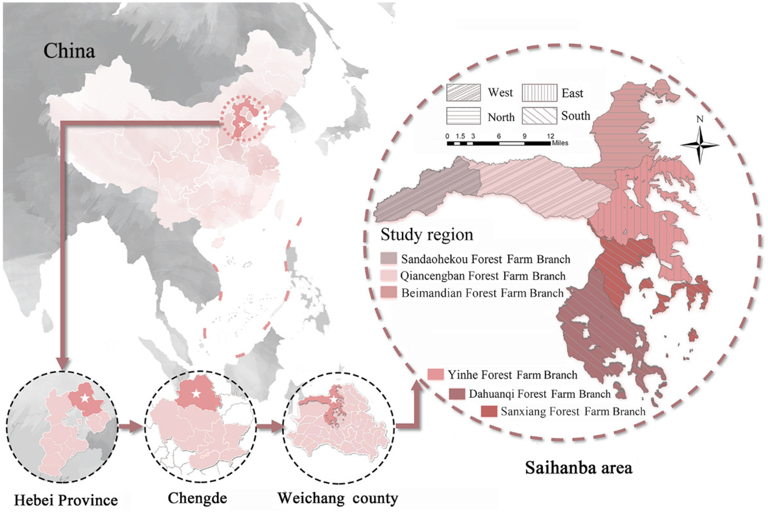
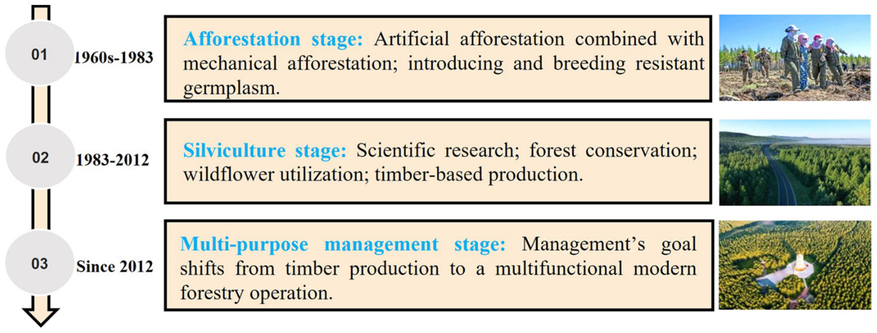
2.1. Study Area

SHB Forest Farm is located in Weichang county, Chengde city, Hebei province, China (42°4′–42°36′ N, 116°53′–117°39′ E), on the southern edge of the Hunshandake Sandy Region in Inner Mongolia [35] (Figure 1). The study area includes six subfarms and 30 operational areas, covering approximately 933.33 km2. The elevation ranges from 1010 to 1940 m. The region has a typical semiarid and semihumid cold temperate continental monsoon climate with an average annual temperature of −2.7 °C and an average annual precipitation of 460.3 mm [36]. Over the past 50 years, the local government and forest managers of SHB have actively explored and implemented the restoration strategies of the “Integrated Management of Mountains, Water, Forests, Farmland, and Lakes”. It has continuously promoted the construction of key ecological projects, and the quality of the ecological environment has shown a trend toward stability and improvement. The deteriorating trend of various natural ecosystems has been basically curbed, and the ecological security barrier framework has been constructed [31]. Reviewing SHB’s development history (Figure 2), although significant ecological construction achievements have been made, continuing large–scale and high–density afforestation work due to the characteristics of artificial forest ecosystems and against the background of global climate change may lead to soil degradation and a decline in the water retention capacity of the ecosystem, posing many risks that could affect its future sustainable development.

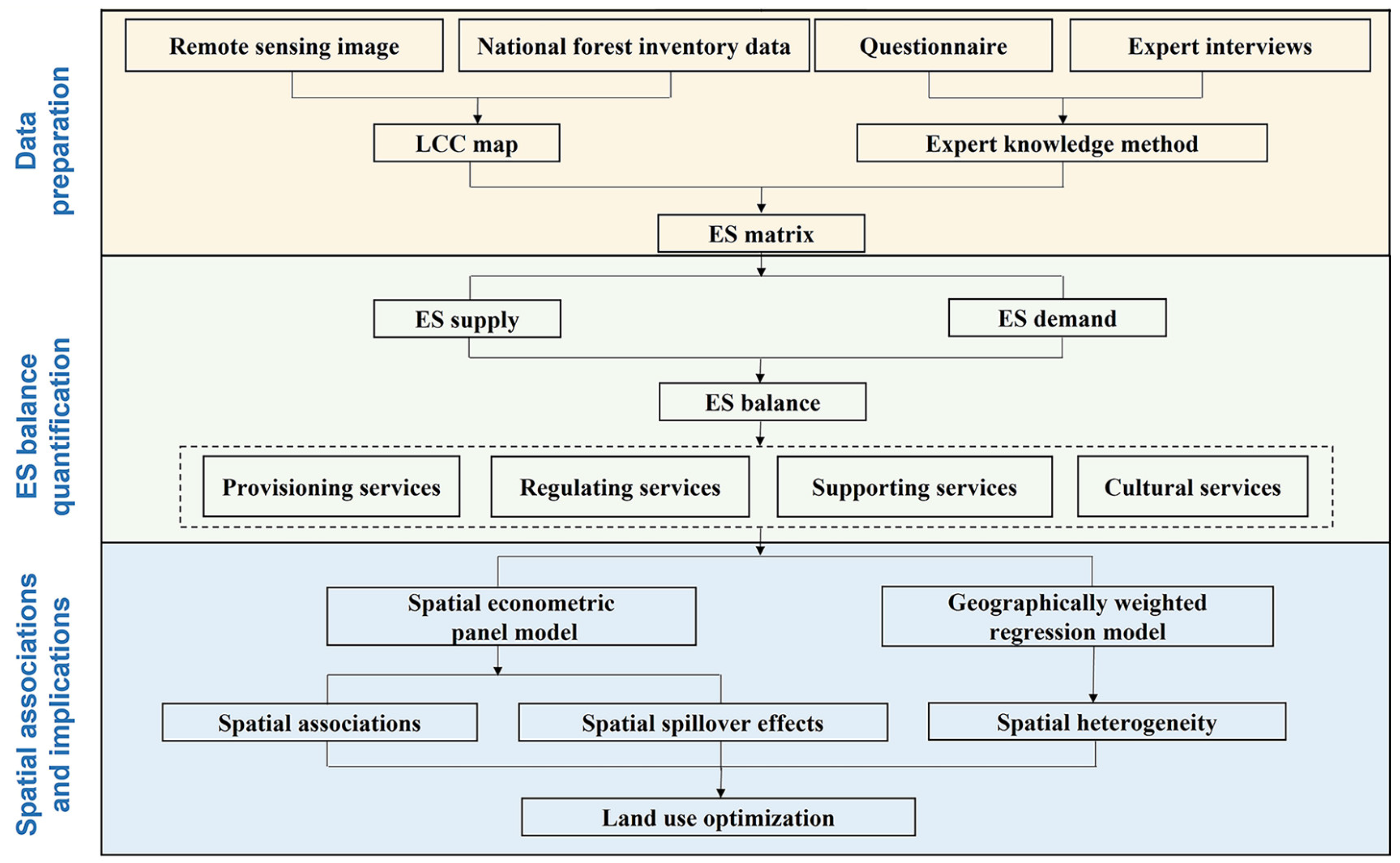
2.2. Conceptual Framework

The ES balance reflects the stability of ecosystems and plays a vital role in maintaining environmental carrying capacity [14,15,26]. The evolution of ecosystems usually has a direct impact on the ES balance [26]. There are two situations of ES imbalance, namely ES surplus (i.e., oversupply) and ES deficit (i.e., the supply is inadequate to meet the demand) [37]. The ES surplus is generally caused by large–scale afforestation and/or secondary afforestation on existing forestlands. Although large–scale afforestation can increase vegetation coverage, it may cause a reduction in cultivated land and wetland areas, leading to a decrease in water conservation and agricultural economic benefits [38,39,40]. By contrast, the ES deficit is typically caused by excessive human intervention and deforestation, which can temporarily increase food production and economic benefits but lead to ecosystem degradation [9,41]. Since the land is covered by a high percentage of forest, the status of the study area is typically ES surplus. To maintain the local supply–demand balance of the ES, effective policy and technical interventions should be conducted by forestry managers and planners.
The threshold for the ES supply–demand balance can be determined based on the natural environmental conditions (e.g., climate property, soil property, and vegetation types) and social–economic conditions (e.g., productivity) [42]. Considering the uncertainty and complexity of future climate change and human activities, this threshold may vary by location, and the social–economic development pathway also has an impact on it. According to field observation and model simulation, the actual ES supply and demand can be evaluated and adjusted quantitatively [43]. Based on the ES balance, the ERPs’ landscape configuration can be adjusted and planned. [44] For example, excessive afforestation can exhaust soil and water resources and lead to increased ecosystem degradation. Therefore, the proportion of woodlands, grasslands, and wetlands in the study area should be carefully coordinated [39]. Furthermore, to ensure sufficient food supply and the livelihood of local farmers, the proportion of cultivated land must also be kept reasonable [40]. Collectively, the forestry managers should opportunely observe the ecosystem’s response to ERPs and the dynamic evolution of the ES balance, provide support for decision–making, optimize the ERPs, thus, promoting the sustainable development of the ecological and socioeconomic systems.

2.3. Data and Methods

As shown in Figure 3, the workflow of this study consisted of three parts: (1) data collection and preprocessing, (2) ES balance quantification, and (3) spatial correlation analysis of the ES balance. The practical significance of each part has also been explained (for details, see Section 2.3.1, Section 2.3.2 and Section 2.3.3).

2.3.1. Data Collection and Preprocessing

The original remote sensing (RS) data for SHB’s three periods (2002, 2012, and 2020) were obtained from the European Space Agency Sentinel–2 satellite (with a spatial resolution of 10 m; https://scihub.copernicus.eu/; accessed on 23 May 2022). The original RS images were interpreted using the ENVI software (ver. 5.1, Exelis Visual Information Solutions, Broomfield, CO, USA) to generate local LUCC maps (with six and 17 land use types at primary and secondary levels, respectively; Supplementary Table S1). Next, the accuracy of the ENVI interpretation results was validated and calibrated using the forest resource survey data from the same periods, and the overall accuracy of the interpretation was >93%, which meet the accuracy requirement for the subsequent ES assessments.
Next, ArcGIS software (ver. 10.2, Environmental Systems Research Institute, Redlands, CA, USA) was used to rasterize the RS images based on the forest resource survey data. To investigate the landscape patterns of the SHB region, the landscape metrics were selected and calculated at the class and landscape levels using FRAGSTATS 4.2.1 software. In detail, patch density (PD), landscape division index (DIVISION), splitting index (SPLIT), and edge density (ED) were selected to represent landscape fragmentation; the Euclidean nearest neighbor distance (ENN) and the patch cohesion index (COHESION) were selected to represent the proximity and connectivity of the landscape, respectively; the interspersion juxtaposition index (IJI) and shape index (SHAPE) were also included in the evaluation system.
Furthermore, socioeconomic factors usually include productivity development level, transportation conditions, cultural and educational status, etc. [23] Wood income is one of the main economic sources of the SHB Forest Farm. Therefore, we chose forest stock volume derived from national forest inventory data as an indirect indicator to reflect the socioeconomic situation of the study area.

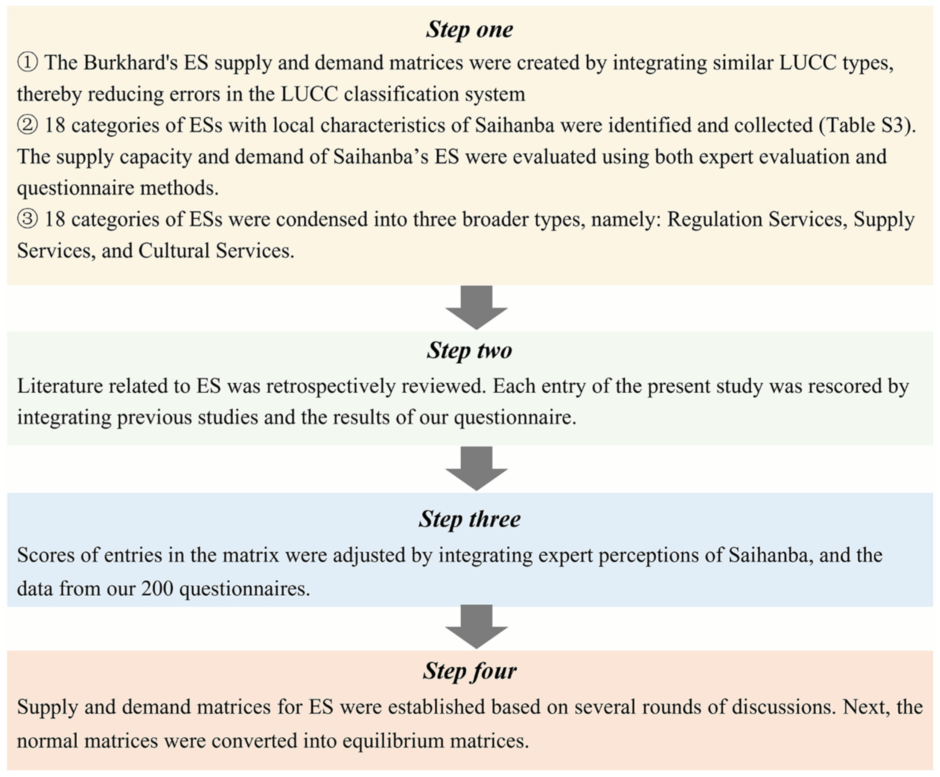
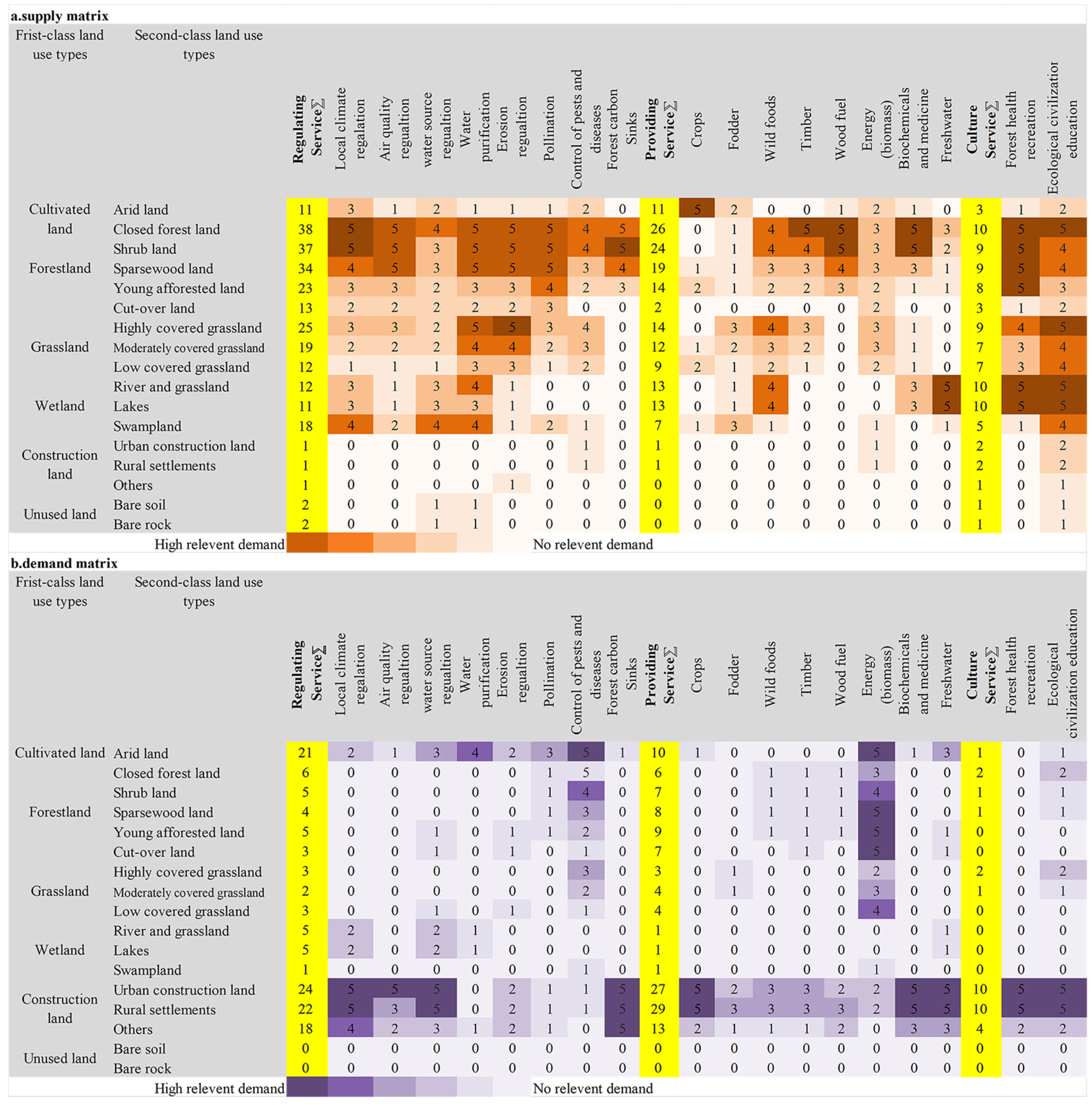
2.3.2. Quantitative Assessment of the Relationship between ES Supply and Demand

Based on the ES matrix method proposed by Burkhard et al. [17,45], the ES balance of the study area in 2002, 2012, and 2020 was quantified. Next, a four–step adjustment framework (Figure 4) was applied to adjust the original matrix using expert knowledge to generate the adjusted supply–demand matrix of ES (Figure 5). The equations for the ES supply index (ESSI), demand index (ESDI), and balance index (ESBI) were as follows:
E S S I = j = 1 m i = 1 n ( L U A i × S i j ) / i = 1 n L U A i
E S D I = j = 1 m i = 1 n ( L U A i × D i j ) / i = 1 n L U A i
E S B I = j = 1 m i = 1 n ( L U A i × B i j ) / i = 1 n L U A i
where i and j represent the types of land use and ES supply, respectively; the m and n represent the total number of the land use and ES supply, respectively; and Sij, Dij, and Bij, respectively, represent the supply, demand, and balance matrix of the No. i land use type’s No. j ES type. LUAi represents the area of the No. i land use type.

2.3.3. Determining the Spatial Correlation between ES Balance and Its Driving Factors

The spatial distribution of landscape patterns may have a significant impact on the supply–demand balance of ES [46]. To improve the ES balance capacity in a specific ecosystem, it is critical to clarify the ES balance’s driving factors and their linkages to landscape patterns and spatial functions. Landscape metrics (for details, see Supplementary Table S2) can provide key information on the structure composition and spatial configuration of the landscape. Additionally, social–economic indicators can also influence the ES balance to some extent [23,47]. In the present study, FRAGSTATS software [48] was used to calculate landscape indicators. To explore the spatial autocorrelation of the local ES, three types of spatial panel models (SPMs) were employed in this study (Table 1), including the Spatial Durbin Panel Model (SDPM), the Spatial Error Panel Model (SEPM), and the Spatially Lagged Panel Model (SLPM).
SDPM reflects the direct effect of independent variables, as well as the indirect effects of neighboring units, on the local dependent variable (i.e., spillover effects). The SDPM is expressed as follows:
Y i = α i = 0 N w i j Y j + φ X i + μ i + ε i
where Yi represents the No. i unit’s ES (i = 1, 2,…, N); α is the autoregressive coefficient; wij denotes the weighted matrix; Yj represents the No. j unit’s ES (j = 1, 2,…, N); and Xi is the independent variable in the ith unit at time. φ represents the vector of coefficients of Xi; μi denotes the spatial effect item; and εi is the error term.
The SEPM accounts for the interaction between local and neighboring units due to omitted variables. The formulas are as follows:
Y i = φ X i + μ i + ϕ i
ϕ i = γ j = 1 N w i j ϕ i + ε i
where  ϕ i  and  γ , respectively, represent the autocorrelation error term and its autocorrelation coefficient.
SLPM considers the spatial lag effect of the independent variable, which is expressed as follows:
Y i = α i = 0 n w i j Y j + φ X i + λ j = 1 N w i j X j + μ i + ϵ i
where λ represents the autocorrelation coefficient.
The variance inflation factor (VIF) was also conducted to detect autocorrelation and reduce collinearity among variables, thereby minimizing redundancy of socioeconomic and landscape indicators (Table 1). The VIF values of all independent variables in this study were <10, indicating low collinearity among the data, which meets the precision requirements of subsequent analysis.
Geographically weighted regression (GWR) is a powerful strategy for simulating heterogeneous spatial processes and is broadly used to capture unique characteristics hidden behind the global, which can also capture spatial features associated with landscape indicators and/or socioeconomic indexes [49]. Thus, combining the results calculated by SPMs, GWR was further applied to investigate the spatial heterogeneity between the ES indices, landscape indicators, and socioeconomic index. The equation involved in the GWR calculation process is as follows:
Y   ( O i , P i ) = β 0 O i , P i + i = 1 k β i O i , P i X i + δ O i , P i
where ( O i , P i ) = denotes the spatial coordinates of the ith unit; Y ( O i , P i )  represents the ESBI predicted value of the ith unit; K is the number of independent variables; βi represents the ith unit’s regression coefficient;  X i  is the landscape and socioeconomic indicators of the ith unit; and δ ( O i , P i )  represents the error term.
The GWR parameters for each unit were calculated as follows:
β ^ O i , P i = X T W ( O i , P i ) 1 X T W ( O i , P i ) Y
W i j = e x p 0.5 d i j / r 2
where W  ( O i , P i )  denotes a spatially weighted diagonal matrix of the ith unit; X and Y denote the independent and dependent variables, respectively;  d i j  represents the Euclidean distance between the sampling jth unit and the predicted ith unit; and r is the bandwidth parameter. In the present study, we performed the modified Akaike information criterion (AIC) [50] to determine the model’s relative efficiency and to select a criterion.
Moran’s I method was also employed to identify the spatial autocorrelation of the supply–demand balance in the local ES balance. This statistical method can accurately reflect the spatial dependence and aggregation among the variables [51]. The associated equations are as follows:
Moran I = i = 1 n j = 1 n w i j ( x i x ) ( x j x ) S 2 i = 1 n j = 1 n w i j
where n represents the number of operational areas or units; S = 1 / n i = 1 n ( x i x ) 2 ; i and j denote two different units or areas, respectively; xi and xj represent the ESSI, ESDI, or ESBI values of the No. i and No. j units/operational areas, respectively; Wij denotes the spatial weight matrix of the ijth unit; and  x  is the mean of the ES balance index of the region. Moran’s I < 0, >0, and =0 represent negative, positive, and no correlation at the spatial level, respectively.

3. Results

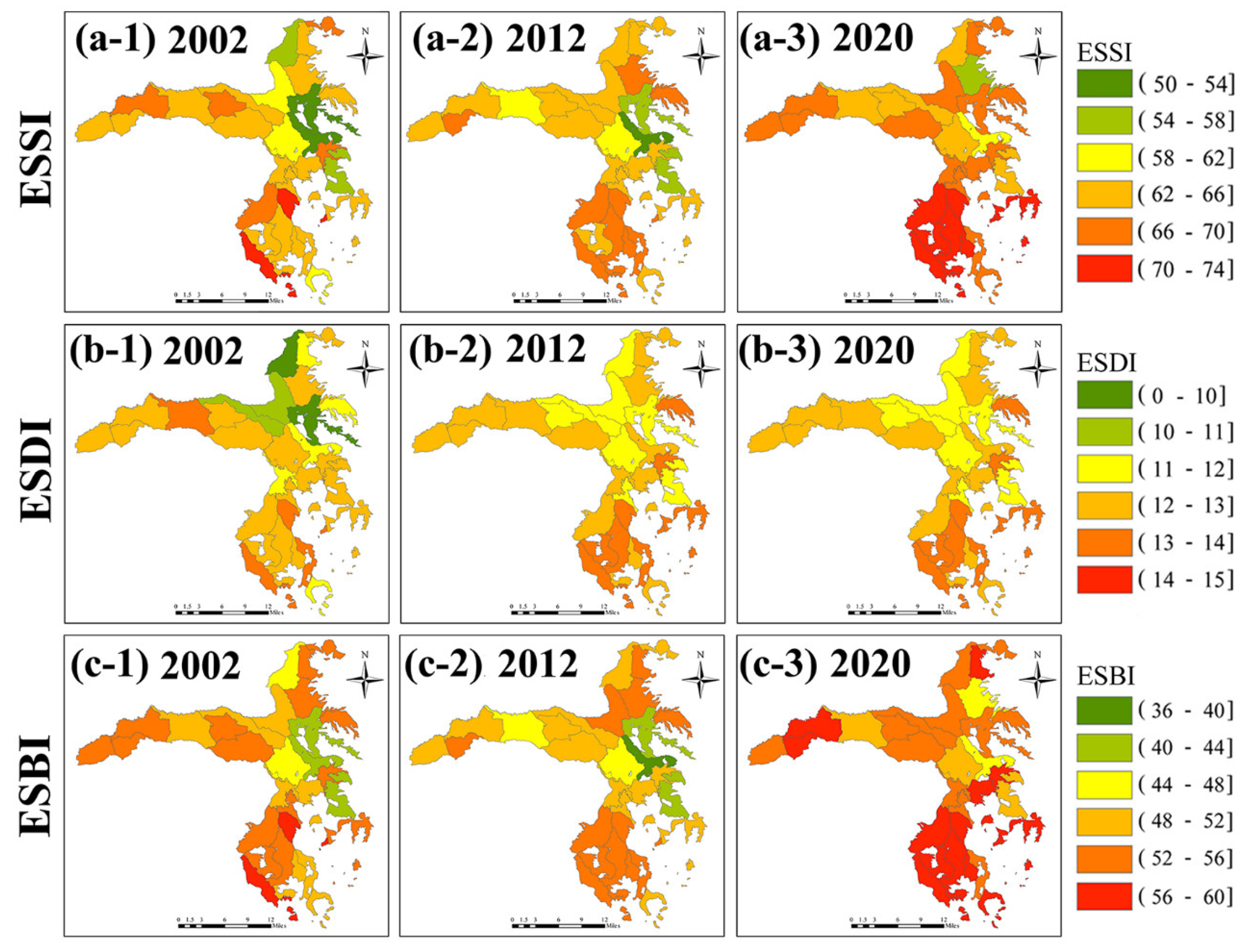
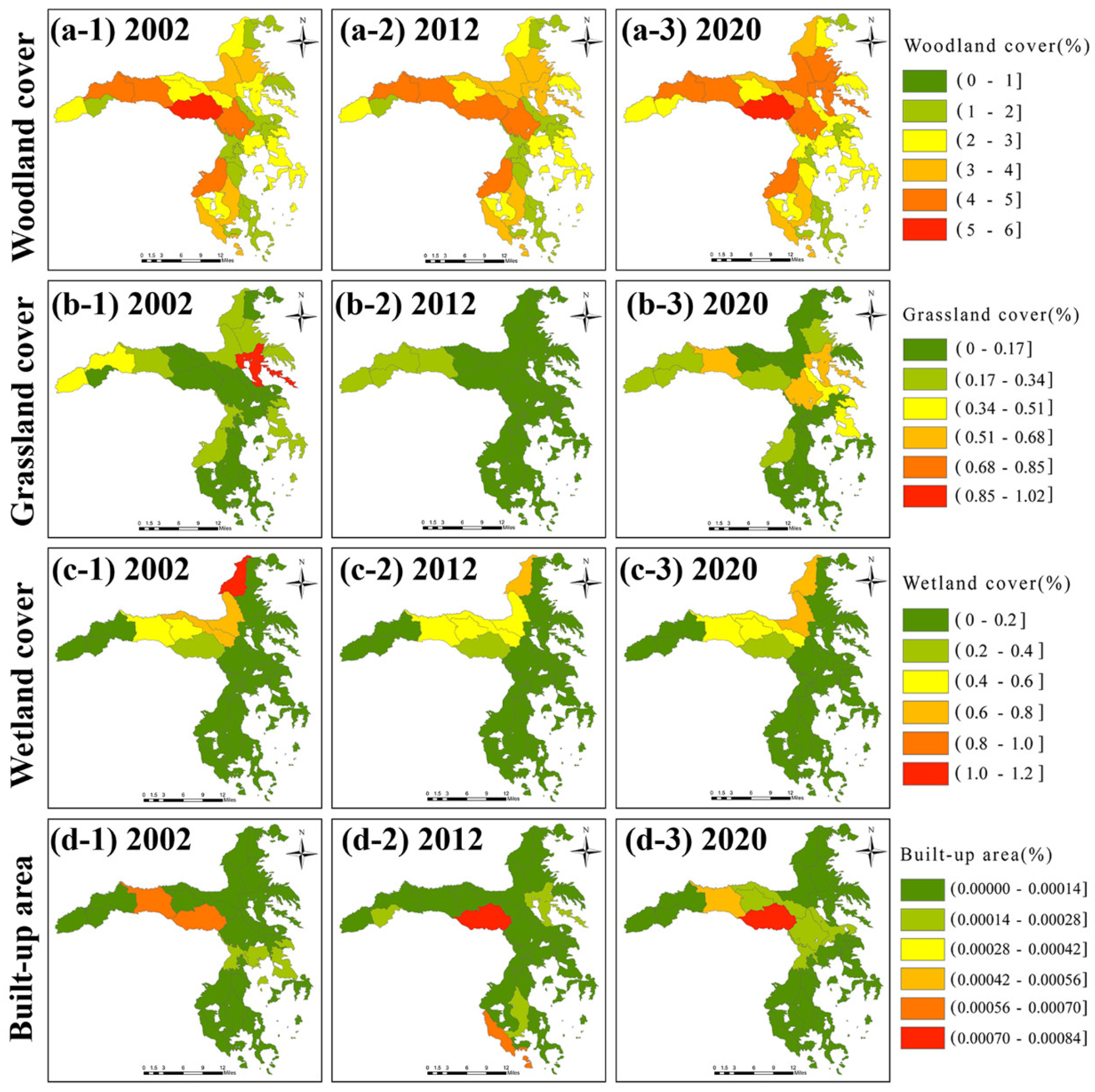
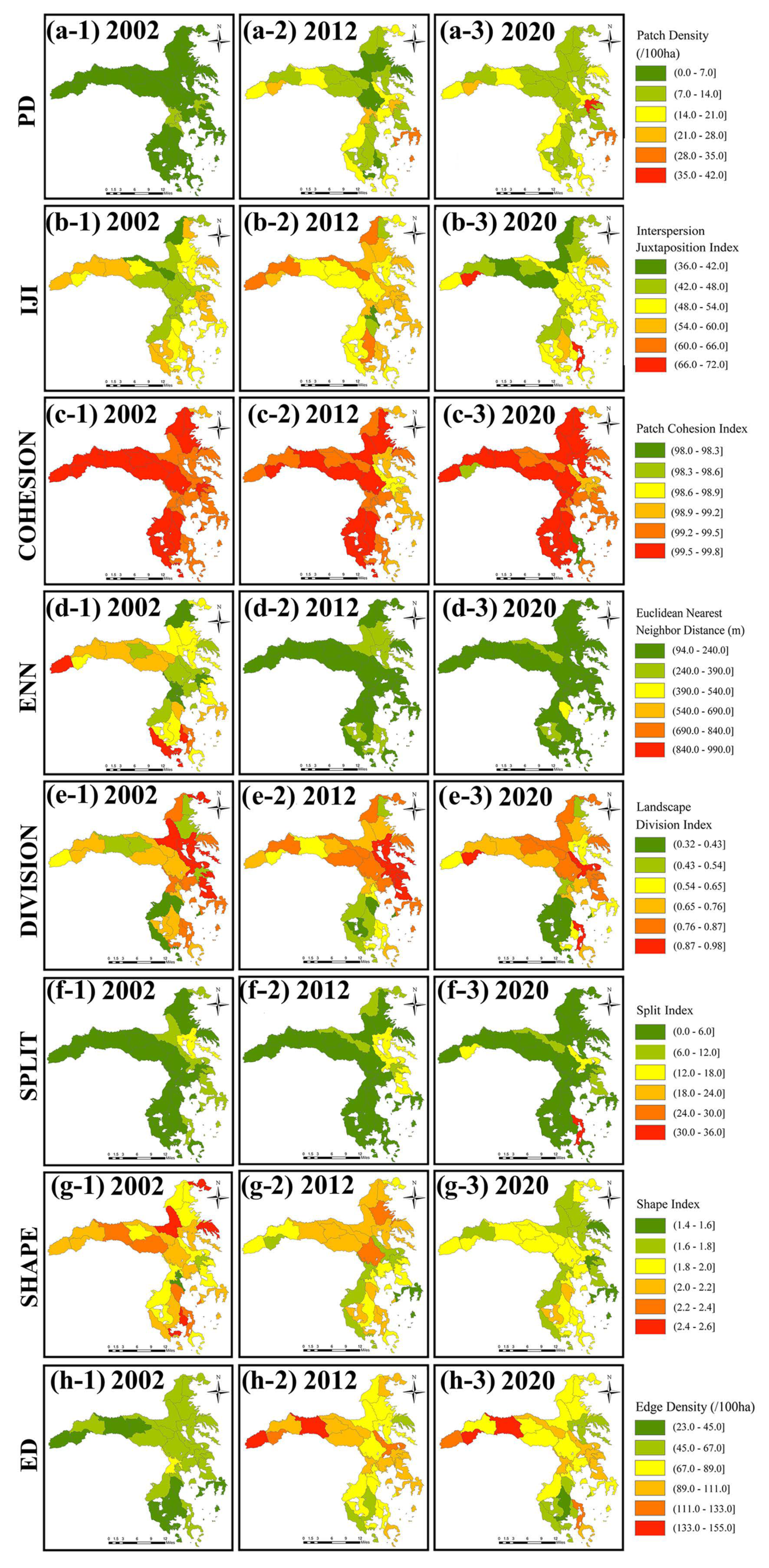
3.1. Spatiotemporal Variations of ES Balance, LUCC, and Landscape Patterns

The area of high ES index in the study region exhibited a gradually increasing tendency from 2002 to 2020 (Figure 6). In detail, the ESSI was higher (62–74) in the southwest and lower (<58) in the east. Meanwhile, the ES supply capacities both increased rapidly in the two areas from 2012 to 2020, and the ESBI showed a similar pattern. The ESDI was higher in the southeast (11–15) but consistently lower in the northern region due to its low proportion of built–up land. The study region has demonstrated an ES surplus, as indicated by the consistently non–negative values of the ESSI, ESDI, and ESBI indices, regardless of whether they were evaluated in terms of space or time. Additionally, from 2002 to 2020, the degree of ES surplus in the region has shown a continuous increase. (Figure 6).
From 2002 to 2020, the proportion of forestland witnessed a gradually increasing trend. In contrast, the proportion of unused land as well as wetland continued to decrease during this period (Supplementary Figure S4). The results of the spatial patterns of major forest types in SHB demonstrated that the proportions of woodlands, grasslands, and built–up land were also gradually increasing, while the proportions of wetlands showed a downward trend (Figure 7). Moreover, in forests, dense forests showed a continuous upward trend, while sparse forests and young forests showed a gradual downward trend, and shrub forests showed no significant changes from 2002 to 2020 (Figure S1).
Furthermore, multiple landscape metrics in SHB showed a significant variation from 2002 to 2020 (Figure 8). In particular, the ENN and SHAPE indexes in the southwest region significantly decreased from 2002 to 2020. In contrast, the PD and ED indexes significantly increased. However, the variations of COHESION and SPLIT were not significant.

3.2. Associations between ES Balance and LUCC, Landscape Pattern, and Socioeconomic Indicators

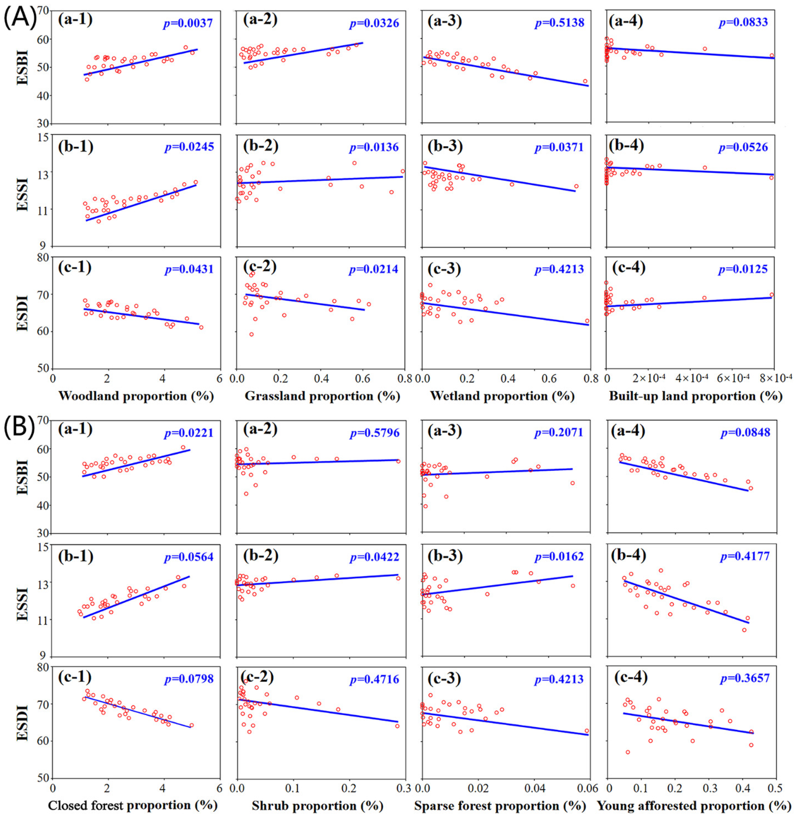
3.2.1. Correlation Analysis between ES Balance and LUCC

The ESBI and ESSI indexes were positively correlated and the ESDI was negatively correlated (p < 0.05) with the proportions of woodlands and grasslands. Wetland proportions were negatively correlated with all three indexes, while the built–up proportion was positively correlated with ESDI and negatively correlated with ESBI and ESSI (Figure 9).
The ESBI and ESSI indexes had a positive correlation, while the ESDI showed a negative correlation with the proportions of closed forest, shrub, and sparse forests. All three indexes were negatively correlated with the young forest proportion.

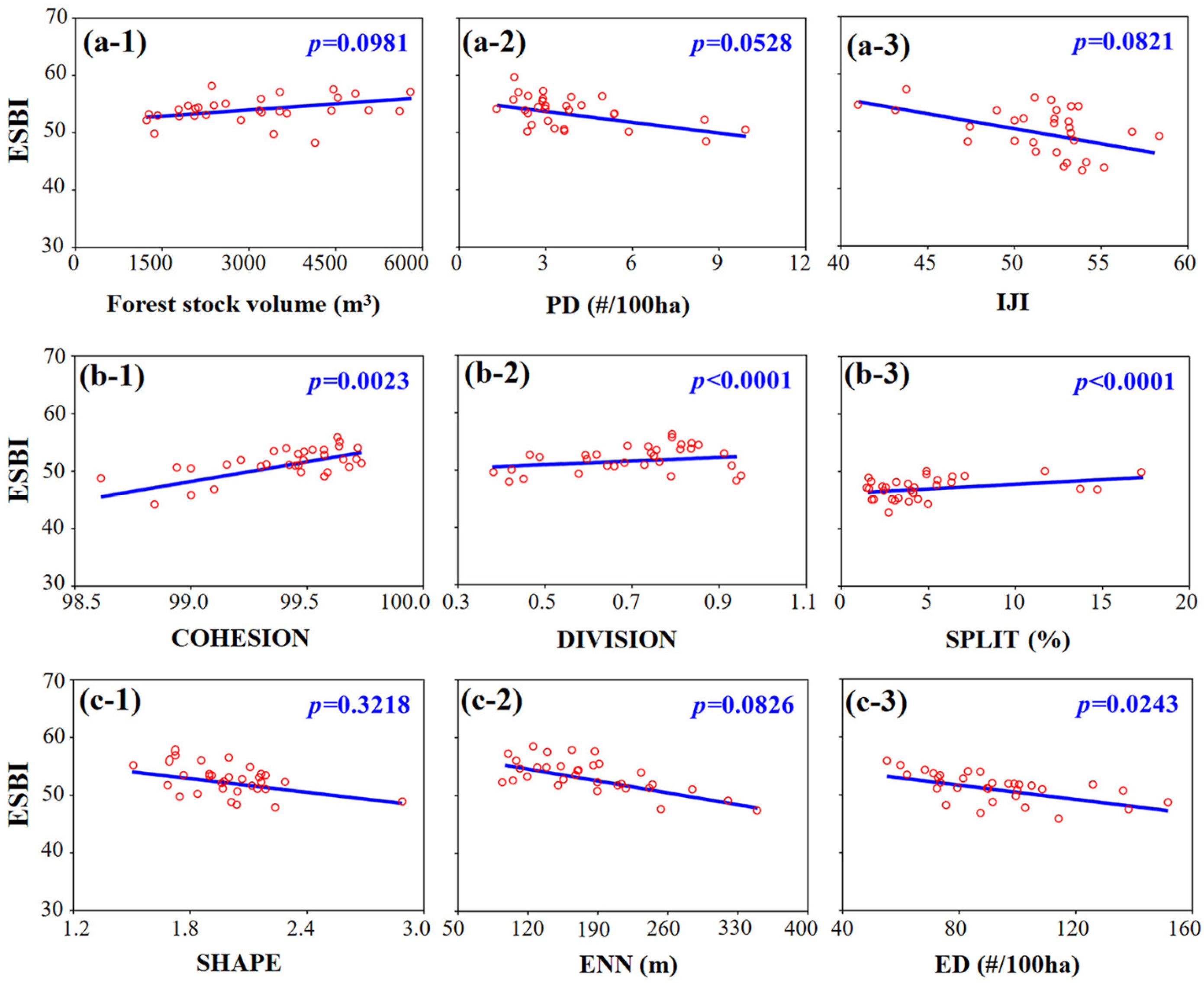
3.2.2. Correlation between ES Indices and Landscape and Socioeconomic Variables

ESSI and ESBI were positively correlated with landscape indicators such as COHESION, DIVISION, SPLIT, and forest stock volume (Figure 10 and Supplementary Figure S2). However, they were negatively correlated with IJI and ENN. As for ESDI, it was positively correlated with most of the landscape indicators, except for IJI, SHAPE, and ENN (Supplementary Figure S3).
Three types of SPMs were used to validate the results of the correlation analysis (Figure 10 and Supplementary Figures S2 and S3). Table 2 shows that as DIVISION increased by 1%, the SLPM–STPFE, SDPM–SFE, and SDPM–STPFE increased by 9.644%, 3.880%, and 16.364%, respectively. By contrast, as ENN increased by 1%, the SEPM–STPFE, SDPM–SPE, and SDP–STPFE decreased by 0.004%, 0.008%, and 0.010%, respectively. These results were consistent with the fitting curve’s trends (Figure 10 and Supplementary Figures S2 and S3), suggesting the high precision of the correlation analysis.
Furthermore, the SDPM model was also performed and identified significant spillover effects of the independent variables (Table 3). In detail, when SHAPE increased by 1%, the ESBI decreased by 0.037% in the present unit and 0.121% in adjacent units. As IJI increased by 1%, the ESBI in the present unit and adjacent units decreased by 0.011% and 0.526%, respectively. Similarly, as SHAPE increased by 1%, the ESBI in the present unit and adjacent units decreased by 0.037% and 0.121%, respectively. In contrast, DIVISION and SPLIT had a positive impact on the present and adjacent units.
The spatial heterogeneity of the driving factors of ESBI was further determined by ordinary least squares (OLS) and GWR models. Supplementary Table S4 shows the R2 and AIC values were both higher in the GWR model than in the OLS model, indicating the GWR model achieved a well–fitting feature. Furthermore, as shown in the results conducted by the GWR model (Supplementary Table S5), the landscape indicator SPLIT had a positive impact on the supply–demand balance of ES; it increased from 0% to 100% from 2012 to 2020. In contrast, the ED index witnessed an opposite trend compared to SPLIT; it decreased from 100% to 56.67% from 2002 to 2020. The ENN index rapidly increased from 0% to 70% during 2002–2012 but slowly reached 100% from 2012 to 2020.

4. Discussion

4.1. Spatial Association between the ES Balance and LUCC

Our data demonstrated a strong correlation between the ES balance and land use type (Figure 9A). The operational area, which had a high proportion of forest land, possessed a high ability for ES supply. In contrast, the operational area with a high proportion of built–up areas had high demand but insufficient supply of ES. The closed forests had significant effects on the ES indexes and enhanced the capacity of ES supply (Figure 9B). However, large–scale afforestation could reduce the local capacity for soil and water conservation [39,40]. Therefore, it is necessary to avoid radical reforestation or afforestation during optimization processes to maintain a stable ES balance. Excessive human interventions can also cause landscape fragmentation, leading to secondary disasters such as wetland degradation [46,52,53]. To effectively coordinate the conflict between human intervention and ecosystem conservation, a spatially explicit model can be utilized to optimize land use allocation. Furthermore, to avoid ES imbalances in the future, the local government and forestry managers in SHB should conduct a series of forest management strategies, including converting sparse forest to dense forest, reducing the proportion of built–up land, and promoting the proportions of forestlands and grasslands.
It is essential to maintain an appropriate proportion of wetlands in rapidly developing Forest Farms [54]. In the future, SHB should prioritize implementing ecological protection and restoration projects, such as wetland protection, returning farmland to wetlands, and restoring fields to lakes. SHB should also comprehensively clean up any construction facilities that negatively impact the native environment and wetland development to ensure the ecological flow of rivers and lakes. In addition, restoration of degraded and sanded riverbanks and lakeshores can be achieved through various methods, including sequestration, afforestation, planting grass, and prohibiting the construction of operational development projects. By adopting these approaches, SHB can avoid future water resource challenges and ensure the preservation of wetlands, prevent sandy lands from shifting southward, and maintain the essential functions of ES.
Notably, the landscape or ecosystem with high biodiversity is more stable and can provide more ecological services, including water cycle, soil conservation, and climate regulation [55]. Thus, it is essential to improve landscape connectivity and heterogeneity so as to maintain high biodiversity. As a result, forest managers should reduce the area of pure forests and increase the proportion of mixed forests to avoid forest degradation. At the same time, to reduce the economic cost of the local afforestation practices in the future, it is essential to consider using more native tree species, such as Larix gmelinii (Rupr.) Kuzen., Pinus sylvestris var. mongholica Litv., Betula platyphylla Sukaczev, and Picea asperata Mast. Meanwhile, the concentration and continuous distribution of the built–up areas should be avoided. Thus, the ecological corridors, ecological networks, and ES supply of the SHB can be optimized, and the connectivity of the landscape and the stability of the ecosystem can be ensured. In addition to the aforementioned measures, to achieve ES balance and multifunctional operation development in the overall region of SHB, the functional connections between ecological corridors should be enhanced to boost local cultural, recreational, and educational services. These optimization measures can also contribute to the ES balance within the framework of integrated development in the Beijing–Tianjin–Hebei region, China.

4.2. Spatial Association of the ES Balance with Landscape and Socioeconomic Variables

The spatial association of the ES balance with landscape and socioeconomic indexes reflect an essential role in landscape allocation and planning for environmental conservation and regional development [56]. The structural and evolutionary characteristics of the landscape can typically affect its associated ecosystem evolution processes, including energy cycling, nutrient transport, and species migration. These processes may, in turn, influence the supply–demand balance of ES [57,58].
In this study, landscape indicators such as NP, IJI, and COHESIVE were used to represent landscape fragmentation, complexity, and physical connectivity, respectively [59,60]. Landscape fragmentation in some areas of SHB reflects intense human intervention, which usually has a negative effect on ESBI (Table 2). Our results showed a significant positive correlation between COHESIVE, DIVISION, SPLIT, and ESBI (p < 0.01; Figure 10), indicating that improving landscape connectivity and diversity is conductive to the formation of ES, leading to an increase in ESBI. The southwest region of SHB had implemented the most vigorous measures, including multiobjective forest management, conversion of natural secondary forests to plantation forests, and clear–cutting of small forest areas, which could well explain the observed patterns. Specifically, the conversion of natural secondary forests to plantation forests may result in a normalization of patch shape and a decrease in spatial diversity. Clear–cutting of small areas of forest may result in an increase of the patch number, leading to landscape fragmentation. Collectively, human interventions may cause increased fragmentation of the landscape in specific areas, highlighting the importance of moderate forest management to maintain a stable and healthy ecosystem.
The results showed that the growth in forest stock volume had increased both ES demand and supply, thus contributing to the supply–demand balance of the ES (Figure 10). Landscape indicators and the forest stock volume index were the primary determinants that affected the ES balance of the study area. Therefore, SHB should optimize the existing landscape structure and land use planning. The SPMs clarified that both landscape metrics and socioeconomic variables affected the supply–demand balance of ES (Table 2). The spillover effects for the independent variables were spatially autocorrelated in the adjacent regions and were also closely related at both physical and economic levels (Table 3). Additionally, the ES balance of SHB was not only affected by the local landscape indexes (i.e., direct impacts) but also influenced by independent factors of the adjacent regions (i.e., indirect impacts; Table 3), possibly due to progressive assimilation or interconversion of adjacent land use types. To avoid an ES imbalance in the future landscape planning and ecosystem protection of SHB, the spillover effect between operational areas should be considered and the management approach of each subfield should be integrated.

4.3. Considering Spatial Heterogeneity and Spillover Effects into ES Decision—Making

In SHB, environmental conditions in one operational area can affect local ecosystems directly or indirectly (Table 3). For example, large–scale and high–density afforestation in a single operational area implies a substantial ecological water demand. Additionally, with rising temperatures, ground evapotranspiration is likely to increase, which may weaken the water–holding capacity of adjacent ecosystems. As one of the origins of the Luan River and Liao River (Figure 1) [35,36], the aforementioned changes in the SHB region may lead to a reduction in the water supply capacity of downstream areas. Therefore, considering the spillover effects and the interdependence between operational areas, ecosystem management and landscape planning must adequately and reasonably allocate landscapes within and between units to mitigate environmental degradation. Furthermore, to prevent ES imbalances in future landscape planning and ecosystem protection in SHB, it is essential to consider the spillover effects between operational areas and to coordinate and optimize forest and land use management approaches across different subfarms.
Our data showed that considering the spatial heterogeneity of determinants can effectively address local environmental problems and provide timely and targeted references for decision–making. In terms of GWR coefficients, significant spatial heterogeneity was reflected among the ES indexes, landscape pattern, and social–economic indexes in SHB, which further highlighted the spatial effects of various factors (Supplementary Table S4). This implied that flexible and reasonable adjustments should be made to landscape planning and environmental policies for ecosystem protection based on the natural conditions and dominant driving factors of each subfield in SHB.
Furthermore, our results also indicate that, although forests and grasslands had a high ES supply capacity (Figure 9A), the proportion of these two should be kept at a suitable level because of the constraint on the carrying capacity of water resources. Therefore, considering the spatial heterogeneity of determinants can help solve local environmental issues and offer targeted references for government decision–making.

4.4. Limitations of the Current Studies and Future Research Directions

In this study, we applied land use types as indicators and the ES matrix method as the theoretical basis to quantify the ES balance of SHB. Notably, the existing investigations related to supply and demand relationships are still in the early stage, and there are still shortcomings in the factors affecting the ES balance and the spatiotemporal dynamic of ecosystem evolution. Despite the constraints of the ES matrix method, it is still an effective method for ecosystem evaluation and management [17,45]. To improve the estimation accuracy and achieve a dynamic balance between ecosystem protection and socioeconomic development, it is necessary to introduce more weighted coefficients/socioeconomic indicators (e.g., social composition and regional differences) to link with the ESBI [61]. Identifying the spatial patterns of ES supply, demand, and balance is beneficial for spatial planning, ecosystem management, and land use decision–making. On the one hand, the ES balance can help researchers better understand the impact of human activities on ES and identify whether the current situation satisfies future land use development. In terms of land use policy making, ESBI can serve as a reference to ensure that human activities and land use planning do not lead to further ecological issues [11,12,13,14,15,16]. By using both strategies, landscape planners and decision–makers can more easily identify ecological sensitive and fragile areas and develop targeted improvement strategies.
Regarding the ES balance’s driving mechanisms, in addition to the landscape indicators (Figure 8) and the forest stock volume (Table 1, Table 2 and Table 3) applied in this study, Chen et al. [62] integrated railway density into socioeconomic indicators for analysis and determined its impact on ES balance. Yuan et al. [63] and Sun et al. [64] analyzed the bundling relationships among ES subcategories, revealing multifaceted interactions among different ESs and their driving factors. However, these studies were more dependent on expert knowledge, resulting in high subjectivity in the evaluation results, which inevitably led to inaccuracies.
Furthermore, even within the same ES category, the balance of ES also exhibits spatial heterogeneity. For example, the landscape and socioeconomic indicators associated with the same land use category may differ in terms of ES supply and demand [65], leading to constraints in using the ES matrix method to evaluate ecological system balance. Therefore, when considering the spatial heterogeneity inside and among land use patches, it is necessary to fully consider natural geographical conditions to improve estimation accuracy and meet the specific requirements of the local community, thereby further supporting ecosystem management and landscape planning.

5. Conclusions

In this study, we used an adjusted ES matrix integrated with spatial econometric methods to quantify and map the spatial pattern of the ES balance in the SHB. We revealed the spatiotemporal characteristics of ES supply, demand, and balance. From 2002 to 2020, the capacity of ES supply in SHB increased significantly more than ES demand, resulting in an oversupply of local ES. We clarified that landscape and socioeconomic indexes, especially landscape metrics, had a dominant effect on the local ES balance. In detail, forest stock volume, forest land proportion, and COHESION showed a positive correlation with the ES balance, while SHAPE, IJI, and the built–up area had a negative correlation with the ES balance. We also assessed the correlation and spatial effects between the driving factors of local ES and identified significant effects on the SHB’s ES balance. Furthermore, we proved that the driving factors of local ES not only exhibited scale dependence but also spatial heterogeneity. Accordingly, the findings of this study can provide valuable insights for land use management, as well as for ecosystem conservation. Additionally, it provides a solid foundation for future multifunctional operations in the SHB and promotes the realization of sustainable development objectives.

Supplementary Materials

The following supporting information can be downloaded at: https://www.mdpi.com/article/10.3390/f14061100/s1, Figure S1: Spatial patterns of different forest types in the Saihanba for 2002, 2012, and 2020; Figure S2: Correlations between the ESSI, forest stock volume and landscape, metrics; Figure S3: Correlations between the ESDI, forest stock volume and landscape metrics; Figure S4: LUCC maps of Saihanba for 2002, 2012, and 2020. Table S1: Characteristics of primary and secondary classification system of the LUCC classifications; Table S2: The selected typical landscape indicators of Saihanba; Table S3: Rationales and potential indicators of ecosystem services; Table S4: Assessment of GWR for 2002, 2012, and 2020 in SHB; Table S5: The spatial proportion of the driving factors influencing Saihanba’s ES balance in 2002, 2012, and 2020.

Author Contributions

Conceptualization, C.L. and Z.Z.; methodology, software, visualization, C.L. and L.X.; investigation, data curation, C.L., L.X., D.L., Y.H., J.K., B.P. and X.H.; writing—original draft preparation, C.L. and L.X.; writing—review and editing, Supervision, Z.Z. and L.X. All authors have read and agreed to the published version of the manuscript.

Funding

This work was funded by the Asia Pacific Network for Sustainable Forest Management and Rehabilitation (APFNet) (2021SP2–CHN), and the Hebei Province Key R & D Program of China, grant number 22326803D.

Data Availability Statement

Data is available upon request to the corresponding authors.

Acknowledgments

The authors thank everyone who helped with this study and the anonymous reviewers for their valuable comments. All authors have read and agreed to the published version of the manuscript.

Conflicts of Interest

The authors declare no conflict of interest.

References

  1. Moreno–Mateos, D.; Alberdi, A.; Morriën, E.; van der Putten, W.H.; Rodríguez–Uña, A.; Montoya, D. The long–term restoration of ecosystem complexity. Nat. Ecol. Evol. 2020, 4, 676–685. [Google Scholar] [CrossRef] [PubMed]
  2. Kuuluvainen, T. Forest management and biodiversity conservation based on natural ecosystem dynamics in Northern Europe: The complexity challenge. AMBIO 2009, 38, 309–315. [Google Scholar] [CrossRef] [PubMed]
  3. Tan, P.Y.; Zhang, J.Y.; Masoudi, M.; Alemu, J.B.; Edwards, P.J.; Grêt–Regamey, A.; Richards, D.R.; Saunders, J.; Song, X.P.; Wong, L.W. A conceptual framework to untangle the concept of urban ecosystem services. Landsc. Urban Plan. 2020, 200, 103837. [Google Scholar] [CrossRef]
  4. Hallberg–Sramek, I.; Nordström, E.–M.; Priebe, J.; Reimerson, E.; Mårald, E.; Nordin, A. Combining scientific and local knowledge improves evaluating future scenarios of forest ecosystem services. Ecosyst. Serv. 2023, 60, 101512. [Google Scholar] [CrossRef]
  5. Li, L.M.; Tang, H.N.; Lei, J.R.; Song, X.Q. Spatial autocorrelation in land use type and ecosystem service value in Hainan Tropical Rain Forest National Park. Ecol. Indic. 2022, 137, 108727. [Google Scholar] [CrossRef]
  6. Hanna, D.E.L.; Raudsepp-Hearne, C.; Bennett, E.M. Effects of land use, cover, and protection on stream and riparian ecosystem services and biodiversity. Conserv. Biol. 2020, 34, 244–255. [Google Scholar] [CrossRef] [PubMed]
  7. Brockerhoff, E.G.; Barbaro, L.; Castagneyrol, B.; Forrester, D.I.; Gardiner, B.; González–Olabarria, J.R.; Lyver, P.O.; Meurisse, N.; Oxbrough, A.; Taki, H.; et al. Forest biodiversity, ecosystem functioning and the provision of ecosystem services. Biodivers. Conserv. 2017, 26, 3005–3035. [Google Scholar] [CrossRef]
  8. Wang, D.; Liang, Y.J.; Peng, S.Z.; Yin, Z.C.; Huang, J.J. Integrated assessment of the supply–demand relationship of ecosystem services in the Loess Plateau during 1992–2015. Ecosyst. Health Sustain. 2022, 8, 2130093. [Google Scholar] [CrossRef]
  9. Chen, Y.M.; Zhai, Y.P.; Gao, J.X. Spatial patterns in ecosystem services supply and demand in the Jing–Jin–Ji region, China. J. Clean. Prod. 2022, 361, 132177. [Google Scholar] [CrossRef]
  10. Huang, F.X.; Zuo, L.Y.; Gao, J.B.; Jiang, Y.; Du, F.J.; Zhang, Y.B. Exploring the driving factors of trade–offs and synergies among ecological functional zones based on ecosystem service bundles. Ecol. Indic. 2023, 146, 109827. [Google Scholar] [CrossRef]
  11. Zhang, S.D.; Wu, T.; Guo, L.; Zou, H.T.; Shi, Y. Integrating ecosystem services supply and demand on the Qinghai–Tibetan Plateau using scarcity value assessment. Ecol. Indic. 2023, 147, 109969. [Google Scholar] [CrossRef]
  12. Wei, W.; Nan, S.X.; Xie, B.B.; Liu, C.F.; Zhou, J.J.; Liu, C.Y. The spatial–temporal changes of supply–demand of ecosystem services and ecological compensation: A case study of Hexi Corridor, Northwest China. Ecol. Eng. 2023, 187, 106861. [Google Scholar] [CrossRef]
  13. Wang, Y.Q.; Huang, H.P.; Yang, G.; Chen, W. Ecosystem service function supply–demand evaluation of urban functional green space based on multi–source data fusion. Remote. Sens. 2023, 15, 118. [Google Scholar] [CrossRef]
  14. Wu, J.S.; Jin, X.R.; Wang, H.; Feng, Z. Evaluating the supply–demand balance of cultural ecosystem services with budget ex–pectation in Shenzhen, China. Ecol. Indic. 2022, 142, 109165. [Google Scholar] [CrossRef]
  15. Zhao, C.; Xiao, P.N.; Qian, P.; Xu, J.; Yang, L.; Wu, Y.X. Spatiotemporal differentiation and balance pattern of ecosystem service supply and demand in the Yangtze River Economic Belt. Int. J. Environ. Res. Public Health 2022, 19, 7223. [Google Scholar] [CrossRef] [PubMed]
  16. Wu, X.; Liu, S.L.; Zhao, S.; Hou, X.Y.; Xu, J.W.; Dong, S.K.; Liu, G.H. Quantification and driving force analysis of ecosystem services supply, demand and balance in China. Sci. Total Environ. 2019, 652, 1375–1386. [Google Scholar] [CrossRef]
  17. Burkhard, B.; Kroll, F.; Nedkov, S.; Müller, F. Mapping ecosystem service supply, demand and budgets. Ecol. Indic. 2012, 21, 17–29. [Google Scholar] [CrossRef]
  18. Staes, J.; Broekx, S.; Van Der Biest, K.; Vrebos, D.; Olivier, B.; De Nocker, L.; Liekens, I.; Poelmans, L.; Verheyen, K.; Jeroen, P.; et al. Quantification of the potential impact of nature conservation on ecosystem services supply in the Flemish Region: A cascade modelling approach. Ecosyst. Serv. 2017, 24, 124–137. [Google Scholar] [CrossRef]
  19. Zhao, Y.H.; Wang, N.; Luo, Y.H.; He, H.S.; Wu, L.; Wang, H.L.; Wang, Q.T.; Wu, J.S. Quantification of ecosystem services supply–demand and the impact of demographic change on cultural services in Shenzhen, China. J. Environ. Manag. 2022, 304, 114280. [Google Scholar] [CrossRef]
  20. Yang, M.H.; Zhao, X.N.; Wu, P.T.; Hu, P.; Gao, X.D. Quantification and spatially explicit driving forces of the incoordination between ecosystem service supply and social demand at a regional scale. Ecol. Indic. 2022, 137, 108764. [Google Scholar] [CrossRef]
  21. Villa, F.; Bagstad, K.J.; Voigt, B.; Johnson, G.W.; Portela, R.; Honzák, M.; Batker, D. A Methodology for Adaptable and Robust Ecosystem Services Assessment. PLoS ONE 2014, 9, e91001. [Google Scholar] [CrossRef]
  22. Huang, K.X.; Peng, L.; Wang, X.H.; Deng, W. Integrating circuit theory and landscape pattern index to identify and optimize ecological networks: A case study of the Sichuan Basin, China. Environ. Sci. Pollut. Res. 2022, 29, 66874–66887. [Google Scholar] [CrossRef]
  23. Wilkerson, M.L.; Mitchell, M.G.E.; Shanahan, D.; Wilson, K.A.; Ives, C.D.; Lovelock, C.E.; Rhodes, J.R. The role of so–cio–economic factors in planning and managing urban ecosystem services. Ecosyst. Serv. 2018, 31, 102–110. [Google Scholar] [CrossRef]
  24. Chen, S.L.; Liu, X.T.; Yang, L.; Zhu, Z.H. Variations in ecosystem service value and its driving factors in the Nanjing Metro–politan Area of China. Forests 2023, 14, 113. [Google Scholar] [CrossRef]
  25. Liu, J.; Xu, Q.L.; Yi, J.H.; Huang, X. Analysis of the heterogeneity of urban expansion landscape patterns and driving factors based on a combined Multi–Order Adjacency Index and Geodetector model. Ecol. Indic. 2022, 136, 108655. [Google Scholar] [CrossRef]
  26. Chen, W.L.; Jiang, C.; Wang, Y.X.; Liu, X.D.; Dong, B.B.; Yang, J.; Huang, W.M. Landscape patterns and their spatial associ–ations with ecosystem service balance: Insights from a rapidly urbanizing coastal region of southeastern China. Front. Env. Sci. 2022, 10, 1–20. [Google Scholar] [CrossRef]
  27. Zhang, Z.; Wang, Y.Y.; Wang, Z.X. A Grey–TOPSIS method based on weighted relational coefficient. J. Grey Syst. 2014, 26, 112–123. [Google Scholar]
  28. Liu, L.T.; Yu, S.C.; Zhang, H.J.; Wang, Y.; Liang, C. Analysis of land use change drivers and simulation of different future scenarios: Taking Shanxi Province of China as an example. Int. J. Environ. Res. Public Health 2023, 20, 1626. [Google Scholar] [CrossRef]
  29. Dong, X.S.; Yuan, Q.Z.; Kou, Y.W.; Li, S.J.; Ren, P. Distribution and ecological network construction of national natural pro–tected areas in the upper reaches of Yangtze River. Sustainability 2023, 15, 1012. [Google Scholar] [CrossRef]
  30. Chen, X.; Du, X.; Liu, W.; Wu, M.; Zhang, X. Analysis on restoration impact value model of Saihanba Forest Farm. Int. Core J. Eng. 2022, 8, 88–94. [Google Scholar] [CrossRef]
  31. Wang, S.; Gui, Y.; Xu, X.; Liu, H. Saihanba–ecological protection construction and its impact evaluation on the environment. Acad. J. Environ. Earth Sci. 2022, 4, 32–37. [Google Scholar] [CrossRef]
  32. Li, B.; Zhang, S.; Wang, S.; Ning, L.; Wang, L. Research on the evaluation model of the ecological impact of the Saihanba based on multiple regression. Environ. Resour. Ecol. J. 2021, 5, 39–43. [Google Scholar] [CrossRef]
  33. Liu, B.; Zhang, K.; Luo, H. Evaluation of Saihanba environmental treatment based on Entropy Method. Int. Core J. Eng. 2022, 8, 393–396. [Google Scholar] [CrossRef]
  34. Yuming, L. Natural Reserve and Ecological Conservation Zone. In The Great Wall in Beijing; EDP Sciences: Les Ulis, France, 2022; pp. 146–156. [Google Scholar]
  35. Sun, J.; Li, Y. Remote sensing monitoring of afforestation and its interaction with climate in Saihanba Mechanical Forest Farm in recent 45 years. In Proceedings of the 6th International Conference on Computer Science and Application Engineering, Virtual, 21–23 October 2022; pp. 1–7. [Google Scholar]
  36. Wang, Z. Ecosystem evaluation and prediction based on Saihanba. Environ. Resour. Ecol. J. 2021, 5, 44–49. [Google Scholar] [CrossRef]
  37. Wang, J.; Zhai, T.; Lin, Y.; Kong, X.; He, T. Spatial imbalance and changes in supply and demand of ecosystem services in China. Sci. Total Environ. 2019, 657, 781–791. [Google Scholar] [CrossRef] [PubMed]
  38. Jiang, C.; Yang, Z.; Wen, M.; Huang, L.; Liu, H.; Wang, J.; Chen, W.; Zhuang, C. Identifying the spatial disparities and de–terminants of ecosystem service balance and their implications on land use optimization. Sci. Total Environ. 2021, 793, 148472. [Google Scholar] [CrossRef] [PubMed]
  39. Vadell, E.; de-Miguel, S.; Pemán, J. Large–scale reforestation and afforestation policy in Spain: A historical review of its un–derlying ecological, socioeconomic and political dynamics. Land Use Policy 2016, 55, 37–48. [Google Scholar] [CrossRef]
  40. Doelman, J.C.; Stehfest, E.; van Vuuren, D.P.; Tabeau, A.; Hof, A.F.; Braakhekke, M.C.; Gernaat, D.E.H.J.; Berg, M.v.D.; van Zeist, W.; Daioglou, V.; et al. Afforestation for climate change mitigation: Potentials, risks and trade-offs. Glob. Chang. Biol. 2020, 26, 1576–1591. [Google Scholar] [CrossRef]
  41. Yi, Y.; Liu, H.; Xu, Q.; Yang, Z. The relationship between ecosystem service supply and demand in plain areas undergoing urbanization: A case study of China’s Baiyangdian Basin. J. Env. Manag. 2021, 289, 112492. [Google Scholar] [CrossRef]
  42. Jiang, M.; Jiang, C.; Huang, W.; Chen, W.; Gong, Q.; Yang, J.; Zhao, Y.; Zhuang, C.; Wang, J.; Yang, Z. Quantifying the sup–ply–demand balance of ecosystem services and identifying its spatial determinants: A case study of ecosystem restoration hotspot in Southwest China. Ecol. Eng. 2022, 174, 106472. [Google Scholar] [CrossRef]
  43. Wu, J.; Guo, X.; Zhu, Q.; Guo, J.; Han, Y.; Zhong, L.; Liu, S. Threshold effects and supply–demand ratios should be considered in the mechanisms driving ecosystem services. Ecol. Indic. 2022, 142, 109281. [Google Scholar] [CrossRef]
  44. Cao, S. Impact of China’s large–scale ecological restoration program on the environment and society in arid and semiarid areas of China: Achievements, problems, synthesis, and applications. Crit. Rev. Env. Sci. Technol. 2011, 41, 317–335. [Google Scholar] [CrossRef]
  45. Burkhard, B.; Kandziora, M.; Hou, Y.; Müller, F. Ecosystem service potentials, flows and demands–concepts for spatial locali–sation, indication and quantification. Landsc. Online 2014, 34, 1–32. [Google Scholar] [CrossRef]
  46. Su, S.; Xiao, R.; Jiang, Z.; Zhang, Y. Characterizing landscape pattern and ecosystem service value changes for urbanization impacts at an eco–regional scale. Appl. Geogr. 2012, 34, 295–305. [Google Scholar] [CrossRef]
  47. Venerandi, A.; Quattrone, G.; Capra, L. A scalable method to quantify the relationship between urban form and socio–economic indexes. EPJ Data Sci. 2018, 7, 4. [Google Scholar] [CrossRef]
  48. Kupfer, J.A. Landscape ecology and biogeography: Rethinking landscape metrics in a post–FRAGSTATS landscape. Prog. Phys. Geogr. 2012, 36, 400–420. [Google Scholar] [CrossRef]
  49. Brunsdon, C.; Fotheringham, S.; Charlton, M. Geographically weighted regression. J. R. Stat. Soc. Ser. D Stat. 1998, 47, 431–443. [Google Scholar] [CrossRef]
  50. Hurvich, C.M.; Simonoff, J.S.; Tsai, C. –L. Smoothing Parameter Selection in Nonparametric Regression Using an Improved Akaike Information Criterion. J. Roy. Stat. Soc. B 1998, 60, 271–293. [Google Scholar] [CrossRef]
  51. Moran, P.A. Notes on continuous stochastic phenomena. Biometrika 1950, 37, 17–23. [Google Scholar] [CrossRef]
  52. Zhang, X.; Ning, X.; Wang, H.; Liu, Y.; Zhang, W. Quantitative assessment of the risk of human activities on landscape fragmentation: A case study of Northeast China Tiger and Leopard National Park. Sci. Total Environ. 2022, 851, 158413. [Google Scholar] [CrossRef]
  53. Zhang, Y.; Yin, H.; Zhu, L.; Miao, C. Landscape Fragmentation in Qinling–Daba Mountains Nature Reserves and Its Influencing Factors. Land 2021, 10, 1124. [Google Scholar] [CrossRef]
  54. Ostad–Ali–Askari, K. Review of the effects of the anthropogenic on the wetland environment. Appl. Water Sci. 2022, 12, 260. [Google Scholar] [CrossRef]
  55. Babu, A. Review of the role of the landscape approach in biodiversity conservation. Sustain. Biodivers. Conserv. 2023, 2, 61–86. [Google Scholar] [CrossRef]
  56. Mouchet, M.; Paracchini, M.–L.; Schulp, C.; Stürck, J.; Verkerk, P.; Verburg, P.; Lavorel, S. Bundles of ecosystem (dis)services and multifunctionality across European landscapes. Ecol. Indic. 2017, 73, 23–28. [Google Scholar] [CrossRef]
  57. Zhang, H.; Jiang, C.; Wang, Y.; Zhao, Y.; Gong, Q.; Wang, J.; Yang, Z. Linking land degradation and restoration to ecosystem services balance by identifying landscape drivers: Insights from the globally largest loess deposit area. Environ. Sci. Pollut. Res. 2022, 29, 83347–83364. [Google Scholar] [CrossRef]
  58. Pickett, S.T.; Cadenasso, M.L. Landscape Ecology: Spatial Heterogeneity in Ecological Systems. Science 1995, 269, 331–334. [Google Scholar] [CrossRef]
  59. Xie, X.; Wang, X.; Wang, Z.; Lin, H.; Xie, H.; Shi, Z.; Hu, X.; Liu, X. Influence of Landscape Pattern Evolution on Soil Conservation in a Red Soil Hilly Watershed of Southern China. Sustainability 2023, 15, 1612. [Google Scholar] [CrossRef]
  60. Li, Y.; Geng, H. Evolution of Land Use Landscape Patterns in Karst Watersheds of Guizhou Plateau and Its Ecological Security Evaluation. Land 2022, 11, 2225. [Google Scholar] [CrossRef]
  61. Boerema, A.; Rebelo, A.J.; Bodi, M.B.; Esler, K.J.; Meire, P. Are ecosystem services adequately quantified? J. Appl. Ecol. 2017, 54, 358–370. [Google Scholar] [CrossRef]
  62. Chen, W.; Chi, G.; Li, J. The spatial aspect of ecosystem services balance and its determinants. Land Use Policy 2020, 90, 104263. [Google Scholar] [CrossRef]
  63. Yuan, Y.; Chen, D.; Wu, S.; Mo, L.; Tong, G.; Yan, D. Urban sprawl decreases the value of ecosystem services and intensifies the supply scarcity of ecosystem services in China. Sci. Total Environ. 2019, 697, 134170. [Google Scholar] [CrossRef] [PubMed]
  64. Sun, X.; Tang, H.; Yang, P.; Hu, G.; Liu, Z.; Wu, J. Spatiotemporal patterns and drivers of ecosystem service supply and demand across the conterminous United States: A multiscale analysis. Sci. Total Environ. 2020, 703, 135005. [Google Scholar] [CrossRef] [PubMed]
  65. Luck, M.A.; Jenerette, G.D.; Wu, J.; Grimm, N.B. The urban funnel model and the spatially heterogeneous ecological footprint. Ecosystems 2001, 4, 782–796. [Google Scholar] [CrossRef]
Figure 1. Location analysis map of Saihanba Forest Farm.
Forests 14 01100 g001
Figure 2. Timeline of the development history of Saihanba since the 1960s.
Forests 14 01100 g002
Figure 3. Flowchart for processing the data in the study area.
Forests 14 01100 g003
Figure 4. The generation programs for deriving ES supply and demand matrix by expert knowledge.
Forests 14 01100 g004
Figure 5. Supply (a) and demand (b) matrices of the Saihanba’s ES.
Forests 14 01100 g005
Figure 6. Spatial patterns of (a-1a-3) ES supply, (b-1b-3) demand, and (c-1c-3) balance indexes of Saihanba in 2002, 2012, and 2020. ESBI, ES balance index; ESSI, ES supply index; ESDI, ES demand index.
Forests 14 01100 g006
Figure 7. Spatial patterns of major land use types of Saihanba in 2002, 2012, and 2020.
Forests 14 01100 g007
Figure 8. Spatial patterns of landscape metrics of Saihanba in 2002, 2012, and 2020. PD, patch density; DIVISION, landscape division index; SPLIT, splitting index; ED, edge density; ENN, Euclidean nearest neighbor distance; COHESION, patch cohesion index; IJI, interspersion juxtaposition index; SHAPE, shape index.
Forests 14 01100 g008
Figure 9. Relationships between the ES indexes (i.e., ESBI, ESSI, and ESDI) and (A) dominant land use categories; and (B) forest land use categories. ESBI, ES balance index; ESSI, ES supply index; ESDI, ES demand index.
Forests 14 01100 g009
Figure 10. Correlations between the ESBI and landscape indicators and socioeconomic index (i.e., forest stock volume). ESBI, ES balance index; ESSI, ES supply index; ESDI, ES demand index; PD, patch density; DIVISION, landscape division index; SPLIT, splitting index; ED, edge density; ENN, Euclidean nearest neighbor distance; COHESION, patch cohesion index; IJI, interspersion juxtaposition index; SHAPE, shape index.
Forests 14 01100 g010
Table 1. ESBI and its influencing factors of Saihanba in 2002, 2012, and 2020.
VariablesMean ValueSDMaximumMinimumVIFMoran’s I
ESBI52.3372.72457.53145.965 −0.115 *
ESSI67.6073.29956.95873.125 0.331 **
ESDI12.9140.60211.46314.108 −0.236 *
Forest stock volume3174.6271834.4316914.122309.0413.2140.378 **
PD10.3054.41324.2675.4411.9140.356 ***
IJI52.0434.08563.05945.5852.1680.378 ***
COHESION99.4360.23299.74698.9189.1080.117
DIVISION0.6870.1460.9190.3724.6390.014 *
SPLIT4.9763.24413.5621.5945.2980.173 *
SHAPE5.13417.20397.7761.6222.6060.387 ***
ENN277.97183.673461.424133.2392.157−0.108
ED47.55210.07478.38123.2532.0020.295 ***
Notes: SD, standard deviation; VIF, variance inflation factor; *** p < 0.01, ** p < 0.05, * p < 0.1. ESBI, ES balance index; ESSI, ES supply index; ESDI, ES demand index; PD, patch density; DIVISION, landscape division index; SPLIT, splitting index; ED, edge density; ENN, Euclidean nearest neighbor distance; COHESION, patch cohesion index; IJI, interspersion juxtaposition index; SHAPE, shape index.
Table 2. Spatial associations between ESBI and its related landscape and socioeconomic indexes.
Independent VariablesSLPM–STPFESEPM–STPFESDPM–SFE SDPM–TPFESDPM–STPFE
Forest stock volume0.001 *0.001 *0.001 *0.0000.004 ***
PD0.5320.141 *0.1270.0830.041
IJI0.064 *0.186 ***0.326 ***0.0350.768 ***
COHESION−16.5561.24319.481 *−11.005 ***50.293 ***
DIVISION9.644 **1.9513.88010.862 **16.364 **
SPLIT−0.613−0.1921.461 **−0.858 ***4.912 ***
SHAPE3.507 *−0.0060.015−0.0010.022 **
ENN−0.004−0.005 *−0.008 ***0.001−0.010 ***
ED0.0690.083 **0.146 ***0.0080.312 ***
W–Forest stock volume 0.00010.0000.0003
W–PD 0.147 *−0.105 *−0.054
W–IJI 0.106 *−0.0180.319 ***
W–COHESION 9.093 **0.02115.957 ***
W–DIVISION −1.815−3.017 *−12.244 ***
W–SPLIT 0.951 ***0.332 **2.193 ***
W–SHAPE 0.030 ***−0.0060.041 ***
W–ENN 0.003 **0.0000.002
W–ED 0.0130.030 *0.001
R20.0030.0030.0060.0050.007
Log–likelihood−67.084−0.083−183.957−246.376−174.574
Notes: SDPM, Spatial Durbin Panel Model; SEPM, Spatial Error Panel Model; SLPM, Spatially Lagged Panel Model; SFE, spatial fixed effects; TPFE, time–period fixed effects; STPFE, spatial and time–period fixed effects; PD, patch density; DIVISION, landscape division index; SPLIT, splitting index; ED, edge density; ENN, Euclidean nearest neighbor distance; COHESION, patch cohesion index; IJI, interspersion juxtaposition index; SHAPE, shape index. R2 represents the goodness–of–fit of the model; and W represents the weight of the data. *** p < 0.01, ** p < 0.05, * p < 0.1.
Table 3. Direct and indirect effects of landscape and socioeconomic variables on ESBI.
Independent VariablesDirect EffectsIndirect EffectsTotal Effects
Forest stock volume0.000 *−0.009 *−0.009 *
PD0.057 *1.297 *1.354
IJI−0.011−0.527−0.538
COHESION5.760 *47.719 ***53.479 ***
DIVISION19.959115.727 ***135.686 ***
SPLIT4.956 *23.081 **28.037 **
SHAPE−0.037−0.121−0.159
ENN−0.0020.051 **0.0493
ED0.428 **1.755 ***2.184 ***
Notes: PD, patch density; DIVISION, landscape division index; SPLIT, splitting index; ED, edge density; ENN, Euclidean nearest neighbor distance; COHESION, patch cohesion index; IJI, interspersion juxtaposition index; SHAPE, shape index. *** p < 0.01, ** p < 0.05, * p < 0.1.
Disclaimer/Publisher’s Note: The statements, opinions and data contained in all publications are solely those of the individual author(s) and contributor(s) and not of MDPI and/or the editor(s). MDPI and/or the editor(s) disclaim responsibility for any injury to people or property resulting from any ideas, methods, instructions or products referred to in the content.

