Article

Application of MaxEnt Model in Biomass Estimation: An Example of Spruce Forest in the Tianshan Mountains of the Central-Western Part of Xinjiang, China

1
College of Geography and Remote Sensing Sciences, Xinjiang University, Urumqi 830017, China
2
Key Laboratory of Oasis Ecology of Education Ministry, Xinjiang University, Urumqi 830017, China
3
College of Ecology and Environment, Xinjiang University, Urumqi 830017, China
4
Xinjiang Jinghe Observation and Research Station of Temperate Desert Ecosystem, Ministry of Education, Urumqi 830017, China
5
Institute of Desert Meteorology, China Meteorological Administration, Urumqi 830002, China
*
Authors to whom correspondence should be addressed.
Forests 2023, 14(5), 953; https://doi.org/10.3390/f14050953
Submission received: 14 March 2023 / Revised: 2 May 2023 / Accepted: 2 May 2023 / Published: 5 May 2023
(This article belongs to the Special Issue Advances in Forest Growth and Biomass Estimation)

Abstract

:
Accurately estimating the above-ground biomass (AGB) of spruce forests and analyzing their spatial patterns are critical for quantifying forest carbon stocks and assessing regional climate conditions in China’s drylands, with significant implications for the sustainable management and conservation of forest ecosystems in the Tianshan Mountains. The K-Means clustering algorithm was used to divide 144 measured AGB samples into four AGB classes, combined with remote sensing data from Landsat products, 19 bioclimatic variables, 3 topographical variables, and 3 soil variables to generate probability distributions of four AGB classes using the MaxEnt model. Finally, the spatial distribution of AGB was mapped using the mathematical formulae available in the GIS software. Results indicate that (1) the area under the receiver operating characteristic curve (AUC-ROC) of the AGB models for all classes exceeded 0.8, indicating satisfactory model accuracy; (2) the dominant factors affecting the distribution of different AGB classes varied. The primary dominant factors for the first–fourth AGB classes model were altitude (20.4%), precipitation of warmest quarter (Bio18, 15.7%), annual mean temperature (Bio1, 50.5%), and red band (Band4, 26.7%), respectively, and the response curves indicated that the third AGB model was more tolerant of elevation than the first and second AGB classes; (3) the AGB has a spatial distribution pattern of being higher in the west and low in the east, with a “single-peaked” pattern in terms of latitude, and the average AGB of pixels was 680.92 t·hm−2; (4) the correlation coefficient between measured and predicted AGB is 0.613 (p < 0.05), with the average uncertainty of AGB estimation at 39.32%. This study provides valuable insights into the spatial patterns and drivers of AGB in spruce forests in the Tianshan Mountains, which can inform effective forest management and conservation strategies.

1. Introduction

Global climate change, characterized by an increase in atmospheric CO2, degrades ecosystem function and biodiversity, and even threatens the sustainable development of socioeconomics [1,2,3]. Carbon sequestration, the storage of atmospheric CO2 in plants, soil and other media, can mitigate the negative effects of climate change. Forest ecosystems cover 31% of the land area and have carbon stocks of 652–1146 Pg C [4,5,6], accounting for approximately 33%–46% of the total carbon stocks of terrestrial ecosystems [7,8]. As a crucial quantitative indicator of forest ecosystem structure and function, forest biomass is an important parameter in the construction of carbon stock estimation models, as there is a ratio of 0.5 between forest biomass and carbon concentration [9]. In the modeling of carbon stock estimation models, various factors contribute to the inaccuracy of the model compared to the measured data, also referred to as uncertainty [10]. In addition, the estimation of biomass is one of the significant sources of uncertainty in carbon stock estimation models [11]. Hence, the construction of accurate biomass models is crucial for carbon stock estimation and climate change assessment.
Forest biomass is composed of above-ground biomass (AGB) and below-ground biomass (BGB) [12], with AGB accounting for 70%–90% of total forest biomass and holding 56% of the potential carbon sink under future climate scenarios [13]. In addition, the Global Climate Observing System (GCOS) uses global above-ground forest biomass as one of the 54 key climate variables for ecosystem modeling [14]. Therefore, AGB estimates can provide a better understanding of future forest carbon emissions and sequestration, which can be used to make timely adjustments to forestry management practices according to emission reduction targets. In addition, dynamic biomass monitoring also serves as convincing evidence of the effectiveness of forest management and climate change mitigation [15,16].
Depending on model algorithms, the methodology for estimating AGB can be divided into traditional algorithms (e.g., multiple stepwise regression models) and machine-learning algorithms (e.g., decision tree methods, artificial neural networks, and support vector machines) [17,18,19]. Compared with traditional algorithms, the nonparametric approach of machine learning algorithms can solve well the problems of nonlinearity as well as high-dimensional features and has great potential in estimating AGB. The Maximum Entropy Model (MaxEnt), an Ecological niche model (ENM) based on the maximum entropy theory proposed by Phillips et al. [20], employs species “presence-only” data and relevant environmental information (such as climate, soil, and vegetation index) to predict the probability distribution of species across geographic space. The MaxEnt model is known for its high predictive accuracy and relatively low sensitivity to sample size limitations [21,22,23], making it a widely used machine-learning algorithm for predicting species distribution [24,25,26]. While few applications of the MaxEnt model for estimating biomass have been made to date, notable examples include the work of Saatchi et al. [27], who applied the model to estimate forest biomass in Latin America, South Africa, and Southeast Asia, obtaining an overall mean uncertainty of ±30% for AGB at the pixel scale. Since then, scholars have made further applications in regions such as Mexico [28], the Congo [29], the United States [30,31], and the Brazilian Atlantic Forest [32]. However, the established MaxEnt model for biomass estimation has largely been applied at large scales, such as intercontinental and national scales, with limited applications to small-scale regions. Thus, one of the objectives of this study is to verify the validity of the MaxEnt model for small-scale regional biomass estimation.
According to previous research, biomass can be estimated using two primary types of data: forest structural parameters measured in the field, such as biomass, tree height, diameter at breast height, and storage volume, and remote sensing data. Forest inventory data on large surfaces is the most important information for accurate biomass estimation, but it is labor-intensive and not conducive to dynamic monitoring. Advancements in remote sensing technology have further broadened the scope of available data for biomass estimation, with optical remote sensing, synthetic aperture radar (SAR), and light detection and ranging (LiDAR) being increasingly utilized [33,34,35,36]. Spectral characteristics of remote sensing images vary based on different forest stand; thus, these characteristics can provide insights into biomass values. Therefore, the use of remote sensing data for biomass estimation has become an important form of complementary data for large areas of forest inventory [34,37]. Among optical remote sensing data, Landsat products have emerged as a primary source for forest AGB estimation due to their large coverage, short acquisition time, high measurement accuracy, non-destructiveness, and accessibility as a free remote sensing data source [19]. Vegetation indices, spectral bands, and texture features have been commonly used spectral feature information for biomass estimation [34,38,39]. Additionally, researchers have incorporated auxiliary environmental factors such as topography, bioclimate, and soils into biomass estimation models to limit predicted biomass spatial distributions, reduce spatial uncertainty, and improve estimation accuracy [34,40].
Spruce, a typical zonal vegetation in the Tianshan Mountains of Xinjiang, China. In Xinjiang, spruce forests cover an area of 758,600 ha and have a storage volume of 170,474,400 m3, accounting for 42.33% of the total area (1,791,900 ha) and 50.66% of the total storage volume (336,540,900 m3) of Xinjiang’s arboreal forests (excluding non-wood product forest), making it an important dominant species in Xinjiang’s mountain forests. Spruce forest plays a crucial role in regional soil and water conservation, air purification, carbon balance, and climate regulation [41], and their importance value has a tendency to increase gradually [42]. In this study, we employ a three-step process to estimate the AGB of spruce forests. First, the measured AGB samples are categorized into distinct AGB classes and appropriate environmental variables are selected. Second, the probability distributions of each AGB class are estimated. At last, the spatial distribution map of the AGB is generated and a detailed analysis of the associated uncertainties is carried out. The aim of this study is to generate a spatial distribution map of AGB in spruce forests, analyze the patterns of their distribution and ecological thresholds, and provide a basis for the conservation and sustainable management of forests.

2. Materials and Methods

2.1. Study Area

The Tianshan Mountains, a prominent mountain range situated in central Xinjiang, China, function as a crucial impediment between the Tarim Basin and the Junggar Basin. The range stretches approximately 1700 km in an east-west direction and has a width of 250–350 km in the north-south direction. The climate has significant regional variations due to factors such as the geographical location of the mountains, the east-west trend of the ranges, and the multiple prevailing air currents. In the north-south direction, with the average annual temperature on the northern slopes ranging from 2.5 to 5 °C and 7.5 to 10 °C on the southern slopes [43]; the annual precipitation on the northern slopes amounts to 500–700 mm, while the annual precipitation on the southern slopes is lower than that on the northern slopes, with a difference of more than 150 mm [44]. In the west and east, annual precipitation drops from 600–800 mm to 176 mm, and the average annual temperature is highest in the western region (5–7 °C), followed by the eastern region (4.7 °C) and lowest in the central region (2–3 °C) [45]. In addition, the forest line experiences a gradual rise from west to east, with a corresponding narrowing of the bandwidth [46]. The study area is located within the central-western part of Xinjiang, bounded by geographic coordinates of 42°05′ N~44°38′ N and 79°53′ E ~88°01′ E. Spruce is the dominant species in the study area, growing on the northern slopes of the Tianshan Mountains at elevations of 1400–2800 m, along with Sorbus tianschanica Rupr., Betula tianschanica Rupr., Populus talassica Kom., Aegopodium alpestre Ledeb., etc. The understory soil is mostly mountain grey-cinnamon soil, contributing to the unique ecosystem of the region.

2.2. Calculation of AGB on the Sample Field

In the Tianshan Mountains of the central-western part of Xinjiang, a total of 144 sample plots were established. The location of each sample plot is indicated in Figure 1. The selected forest plots were well-established, were not affected by pests or diseases, and with minimal human disturbance. To gather data from the sample plots, we employed various geospatial instruments. Specifically, we measured the sample circle with a 10 m radius using a high-precision laser rangefinder, recorded the elevation, latitude, and longitude of each plot using GPS, and quantified the number of spruces within the sample circle. Furthermore, we meticulously inspected every tree within the sample plot to acquire the diameter at breast height, and collected the tree height using a laser altimeter.
The determination of forest biomass is often achieved by utilizing allometric relationships that exist between various tree measurement parameters such as tree height (H: m), diameter at breast height (DBH: cm), stand density, storage volume, and other factors [47,48]. In the present investigation, the estimation of AGB for the spruce forest was conducted at the sample scale using the biomass regression equations for different organs, as established by Liu et al. [49] (Table S1). Considering the impact of sample size and variances within AGB classes on model accuracy, the K-Means clustering algorithm, which minimizes intra-cluster variance, was utilized to divide the 144 AGB samples into four AGB classes, as shown in Table 1.

2.3. Processing and Selecting Environment Variables

Landsat 8 OLI images, with a spatial resolution of 30 m, were obtained from the Landsat Collection2 Level-1 dataset from the USGS website (https://www.usgs.gov/, accessed on 18 February 2022). The data was processed using ENVI 5.6 to perform radiometric calibration, atmospheric correction, mosaic, and extraction by mask, among others. To select relevant environmental variables, four vegetation indices were extracted, including the Normalized Difference Vegetation Index (NDVI), Ratio Vegetation Index (RVI), Soil-Adjusted Vegetation Index (SAVI), and Enhanced Vegetation Index (EVI). Additionally, three principal component features of Brightness (BRI), Greenness (GRE), and Wetness (WET), five visible bands (Band 2, 3, 4, 5, and 7), and eight texture feature factors were extracted based on 3 × 3, 5 × 5, and 7 × 7 windows, respectively. These texture features included Mean (MEA), Variance (VAR), Homogeneity (HOM), Contrast (CON), Dissimilarity (DIS), Entropy (ENT), Second Moment (SEC), and Correlation (COR).
The 19 bioclimatic variables used in this study were obtained from the WorldClim Global Climate Database (https://www.worldclim.org/, accessed on 18 February 2022). These variables were derived from monthly temperature and precipitation data and have a spatial resolution of 1 × 1 km. Topographic data, including elevation, slope, and aspect variables, were obtained from the 2020 NASA-released 30 m SRTM DEM (https://earthdata.nasa.gov/, accessed on 18 February 2022). Sand content, clay content, and soil water content (volumetric %) for 33 kPa at 30 cm depth data were obtained from OpenLandMap (https://opengeohub.org/, accessed on 18 February 2022) with a spatial resolution of 250 m. To meet the variable requirements of the MaxEnt model, all the aforementioned data were uniformly sampled to 1 × 1 km spatial resolution using the UTM-WGS84 coordinate system. Finally, the study area was extracted by mask to ensure that only the relevant data were used in the analysis.
The effective selection of environmental factors is a fundamental step in constructing a reliable model, and can prevent the occurrence of issues such as multicollinearity and overfitting that may undermine the accuracy of the model. To achieve this, a two-step approach was employed in this study. Firstly, Pearson correlation coefficients were calculated between the texture feature variables and the 144 AGB samples. Only the texture feature variables that exhibited significant correlation were retained, namely COR2_W5 (R = −0.197, p < 0.05), COR2_W7 (R = −0.202, p < 0.05), COR5_W5 (R = 0.198, p < 0.05), COR5_W7 (R = 0.287, p < 0.01), and HOM1_W7 (R = 0.170, p < 0.05). Secondly, a jackknife test was conducted to determine the contribution of each of the 42 environmental variables (Includes 5 texture feature variables, 4 vegetation index variables, 3 principal component variables, 5 visible wavelength variables, 19 bioclimatic variables, 3 topographic variables, 3 soil variables) in the model. Variables were removed when the percent contribution of the variable was greater than 0.1%. As exceeding the number of available samples may lead to overfitting [50], to ensure optimal model performance, only environmental variables with a high contribution are retained in the 3rd and 4th AGB class models, in amounts equivalent to the sample size. The results of the environmental variables selection process are presented in Table 2.

2.4. Modeling of AGB Estimation

The MaxEnt modeling approach is a widely-used method for predicting the spatial distribution of species and assessing their habitat suitability [51,52,53]. This approach requires three main input data: (1) the location of known species occurrence points, (2) the spatial extent of the study area, and (3) explanatory variables or covariates that describe the environmental conditions at the occurrence points. The MaxEnt model then estimates the probability of species occurrence across the study area by calculating the distribution of “point” probabilities across the image space. The optimal probability distribution is then selected based on the entropy of the predicted probability distribution. The MaxEnt software version 3.4.4 utilized in this study was obtained from the online resource ((https://biodiversityinformatics.amnh.org/open_source/maxent/) (accessed on 8 July 2022)). This software is widely recognized for its robustness and efficiency in species distribution modeling and has been used in numerous ecological studies.
The process of modeling four AGB classes was conducted using rigorous and standardized procedures. The model was run on default settings as follows: random test percentage = 25, regularization multiplier = 1, maximum number of background points = 10,000, and replicates = 10. The replicated run type was set as bootstrap. Ultimately, the average of the ten replications was used as the final result for each AGB class [53,54]. The application of the maximum test sensitivity plus specificity logistic threshold (MSS) for habitat threshold selection ensured objectivity, equivalence, and discriminatory power, while also accounting for potential outliers and sample size limitations [55].To estimate the AGB on each pixel and construct a spatial distribution map of AGB for the study area, the method proposed by Saatchi et al. [27] was utilized (Equation (1)). This approach leverages the distribution probabilities of each AGB class, along with the measured AGB, to generate spatial estimates of AGB. Consistent with Saatchi et al. [27], the root mean square error (RMSE) was calculated and the probability of distribution of each biomass AGB class was introduced to quantify the uncertainty of estimation (Equations (2) and (3)). Through this rigorous methodology, we can be confident in the accuracy and reliability of our spatial distribution map of AGB.
B ^ = i = 1 n P i n × B i i = 1 n P i n
σ B ^ = i = 1 N B i B ^ 2 P i i = 1 N P i
ε p r e d i c t i o n = σ B ^ / B ^ × 100
where B ^ is the predicted AGB value; B i is the median value of each AGB class; P i is the probability of distribution of each AGB class; n is the number of iterations. It was verified that the AGB distribution, as well as the cross-validation results, were optimal when n = 3 [27,28].
To assess the model’s performance, we utilized the widely recognized and independent metric, the Area Under the Receiver Operating Characteristic Curve (AUC-ROC), which measures the model’s ability to accurately predict the spatial distribution of the target species based on environmental variables. A higher AUC value indicates a stronger correlation between the environmental variables and the predicted distribution, resulting in better discrimination between the presence and absence of the target species, as confirmed by numerous studies in the field [56]. The interpretation of the AUC values followed the widely accepted standards, where values ranging from 0.5 to 0.6 denote simulation failure, 0.6 to 0.7 indicate poor performance, 0.7 to 0.8 indicate fair performance, 0.8 to 0.9 indicate good performance, and 0.9 to 1.0 indicate excellent performance.

3. Results

3.1. Evaluation of Model Accuracy

The AUC values obtained from both the training and testing sets of the first–fourth AGB class models were notably above 0.8, indicating a robust model performance (as shown in Table 3). Furthermore, the first and second AGB class models demonstrated particularly high predictive accuracy, achieving AUC values exceeding 0.9. These results demonstrate the effectiveness of the model construction process in generating reliable estimates of AGB. Consequently, all four AGB class models may be utilized with confidence for AGB estimation purposes in these forests.
The accuracy of the first–fourth AGB class model showed an overall decreasing trend with a reduction in sample size. It is noteworthy that the accuracy of the fourth AGB class model, based on a limited number of only seven samples, outperformed the third AGB class model in terms of training and testing AUCs. The size of the sample is a crucial factor that can significantly affect the accuracy of the model. However, the potential bias in the habitat threshold resulting from the disparity in the environmental background between the measured samples cannot be disregarded. Therefore, a more extensive and representative sample is needed to improve the accuracy and robustness of the AGB class model.

3.2. Analysis of Environmental Variables Affecting the Distribution of AGB

The contribution of environmental variables to the construction of the AGB class models was evaluated using the jackknife test embedded in the MaxEnt v3.4.4 software (Table 4). The environmental factor response curves based on the MSS revealed the best ecological niches for species distribution, with values of 0.168, 0.164, 0.395, and 0.439 for the 1st–4th AGB class models, respectively. For the 1st AGB class model, elevation (20.4%, 1370–2564 m), precipitation of warmest quarter (Bio18, 20%, 103–195 mm), precipitation seasonality (Bio15, 12%, 51–87 mm), and soil water content (SWC, 7.8%, 0%–5%) were identified as dominant factors, with a cumulative contribution of 63.2%. The 2nd AGB class model was influenced by precipitation of the warmest quarter (Bio18, 15.7%, 109–202 mm), precipitation seasonality (Bio15, 12.7%, 45–90), and elevation (9.5%, 1343–2806 m). Moreover, slope (12.7%, 5–56°) had a greater impact on the model than elevation. The 3rd AGB class model was strongly influenced by annual mean temperature (Bio1, 50.5%, −3–3 °C), and its suitable elevation range changes dramatically, with a range of 571–3351 m. The 4th AGB class model was primarily driven by remote sensing features such as Band4 (26.7%), HOM1_W7 (16.1%), and COR2_W5 (11.9%), with Band4 and COR2_W5 showing a negative correlation with AGB, while HOM1_W7 showed a positive correlation.

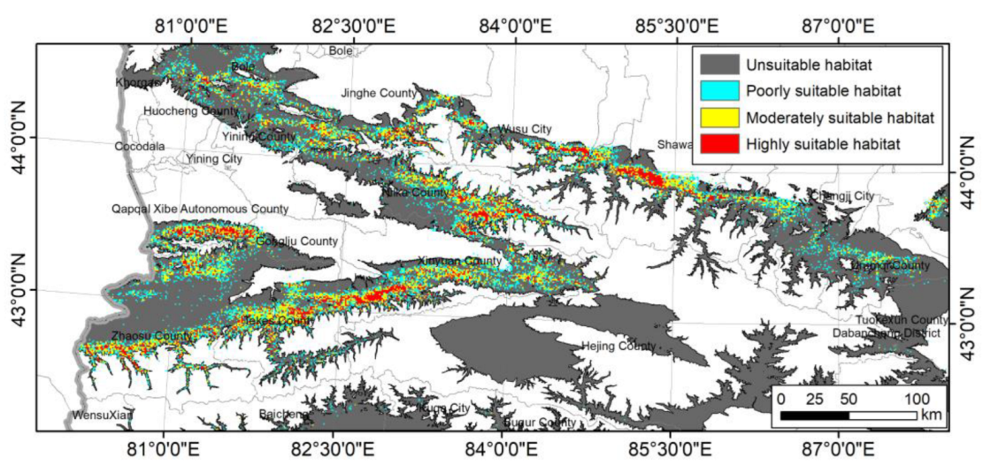
3.3. Spatial Distribution Pattern of AGB

According to the MSS, 0.168, 0.164, 0.395, and 0.439 were used as thresholds of distribution models of first–fourth AGB classes, respectively, and the probability above this threshold was classified into three suitability ranks using the natural breaks (Jenks) method (Figure 2). Suitable areas for first–fourth AGB classes are 11.10 × 10⁶ km2, 83.76 × 10⁵ km2, 19.69 × 10⁶ km2 and 16.81 × 10⁶ km2, respectively. In terms of spatial distribution characteristics, the distribution of the second AGB biomass class is almost extremely low potential in Hutubi County, Changji City, Urumqi County and Zhaosu County compared to the first AGB class. In contrast to the first and second AGB classes, the suitability habitat of the third AGB class expands considerably outwards, with the most notable expansion in the western region (e.g., Bole, Qapqal Xibe Autonomous County, Zhaosu County, China, etc.). Unlike the expansion of the third AGB class, the expansion of the fourth AGB class was distributed beyond the actual distribution of spruce forests (elevation from 1400 to 2800 m) and there was no obvious distribution pattern. The environmental variables involved in the modeling of the different AGB classes are important factors influencing spatial distribution.
Using 100 m as an elevation gradient, the total number of AGB pixels for different elevation gradients was extracted based on ArcGIS 10.4 to analyze the spatial distribution patterns of four biomass classes at elevation; in addition, the observations were compared with the known actual distribution of spruce forests (elevation from 1400 to 1800 m) to analyze the predictive accuracy of the model at a spatial scale. The concentration within the elevation range of 1600–2500 m, as evidenced by the spatial of more than 500 pixels in each AGB class, is a noteworthy result (Figure 3). Moreover, the potential distribution of the third and fourth AGB classes exhibits a spatial propensity to expand towards lower elevations (<1000 m) and higher elevations (>3000 m) when compared to the first and second AGB classes, which can be attributed to the relatively small sample size of the third and fourth AGB classes. The limited number of samples in these classes hinders the accurate characterization of the growth conditions and thereby constrains the accurate delimitation of their spatial dispersal.
As the accuracy of the model was influenced by sample size, all 144 AGB samples and 31 environmental variables (Table S2) were used to predict the spatial distribution of spruce forests (Figure 4), and the results obtained were compared to the spatial distribution of spruce forests on the four AGB classes (Figure 2). Training and test AUCs for the model using all measured AGB samples were 0.97 and 0.93 (Table S3), respectively, and more than 96% of the pixels were located between 1400 m and 2800 m. For the spatial location of highly suitable habitats, the model using the 144 AGB sample is relatively consistent with the first biomass class model. The spatial expansion was most evident at the third and fourth AGB classes when comparing the model using 144 AGB samples with the models at first–fourth AGB classes. In addition, when the 144 AGB samples were spatially overlaid with the distribution of spruce forests (Figure 4), more than 90% of the points fell on suitable habitats. Therefore, we used the model with the 144 AGB samples constructed to extract the area of the four biomass classes.
The average AGB at the pixel scale is estimated at 680.92 t·hm−2, exhibiting spatial variations across different regions (Figure 5). At the pixel scale, the study area consisted of 12395 AGB pixels, with 50% of the pixels falling within the AGB range of 602~1071 t·hm−2, reaching 6259 pixels. The concentration of pixels with AGB values between 602 t·hm−2 and 1071 t·hm−2 was observed in the western regions of the study area, including Zhaosu County, Tekes County, Qapqal Xibe Autonomous County, and Bole City. In contrast, the pixels with AGB values that are lower than 312 t·hm−2 were concentrated in Xinyuan County, Nilka County, and Shawan County. Notably, the counties of Xinyuan and Nilka had high concentrations of pixels with high AGB (≥1071 t·hm−2). Additionally, the Ili River valley’s two sides had concentrated distribution areas of high AGB pixels. Spruce is a species that favors warm and wet conditions, and the unique “trumpet” topography of the Yili River valley, which opens to the west, facilitates the transportation of moisture-laden air from the warm Atlantic Ocean, thereby providing favorable conditions for forest growth. In general, the spatial distribution of AGB exhibits a west-to-east pattern, with the highest AGB values in the western regions and lower values towards the east.
To analyze the relationship between AGB and geographical coordinates in, the study conducted a total count of AGB per 0.01° of latitude and 0.01° of longitude. Linear fit analysis was used to determine the correlation between AGB and longitude and latitude. The results indicate a significant negative correlation between AGB and longitude (R2 = 0.68, p < 0.05) (Figure 6a). The maximum AGB was observed between 81° E–83° E, and decreased gradually towards the east. The total AGB demonstrated a “single-peaked” distribution pattern with latitude, reaching its maximum between 43° N–44° N (Figure 6b). Spruce forest thrives in warm and humid conditions, which are conducive to the full development of forest stands.

3.4. Accuracy and Uncertainty Analysis of AGB Estimation

The 144 measured AGB were extracted and fitted with their corresponding predicted AGB, resulting in a high accuracy with an R-value of 0.613 (p < 0.05) (Figure 7). Comparing the prediction accuracy of different AGB classes, the 1st AGB class showed a poor model simulation accuracy with an average absolute error of 307.39 t·hm−2, an average relative error of 220.34%, and a root mean square error of 208.806 t·hm−2, indicating the presence of the phenomenon of “low value-overestimation”. The R-values of the 2nd and 3rd AGB classes are greater than 0.2; with the R-value of 0.445 (p < 0.05), with the 2nd AGB class showing the best fit with an R-value of 0.445 (p < 0.05), an average absolute error of 150.06 t·hm−2, and an average relative error of 18.21%.
To further investigate the accuracy of the MaxEnt model for AGB estimation, uncertainty was calculated for the entire study area using Equations (2) and (3). Furthermore, the uncertainty distribution was extracted for each biomass class according to Figure 5. The average uncertainty of AGB estimation was 39.32%. The mean uncertainty on pixels was lowest in the first AGB class, specifically, these pixel points were mainly located in Xinyuan and Nilek counties (Figure 8). Mean uncertainty was highest on pixels in the second AGB class (AGB between 312 t·hm−2 and 602 t·hm−2), with high uncertainty values (>60%) on single pixels still partially in Nilek County, consistent with the first AGB class. The number of pixels with uncertainty is greatest in the third biomass class; whereas the fourth biomass class has a significantly reduced number of pixels with uncertainty due to the extraction using the area predicted by the 144 AGB samples.
In addition, the effects of two classification methods on the sample, the K-Means clustering algorithm and interval classification method, on the accuracy of the estimated biomass were compared in the study (Table 5). Compared with the K-Means clustering algorithm, the interval classification method resulted in a smaller improvement in estimation accuracy, with an increase in R-value of 0.026 and a decrease in RMSE of 11.407 t·hm−2. However, the model missed six presence points when using the interval classification method. The results suggest that the K-Means clustering algorithm is more appropriate for partitioning AGB samples, although sufficient sample sizes for each AGB class must be ensured.

4. Discussion

4.1. Dominant Factors Influencing AGB Distribution

Plant growth and productivity are influenced by various biotic and abiotic factors such as topography, temperature, precipitation, and soil. Topography controls the spatial distribution of hydrothermal conditions and soil nutrient accumulation, which subsequently affect plant growth [57,58]. The third AGB class is much more tolerant to altitude than the first and second AGB classes. At high altitudes, the environmental tolerance of plants is mainly manifested in tolerance to minimum temperatures during the growing season, whereas at lower altitudes plants are mainly affected by drought stress, which is more pronounced under global warming; therefore, mid-altitude areas are more suitable for spruce stands with high biomass, as Figure 3 clearly shows [59,60].
The climate is a fundamental environmental parameter that governs spatial heterogeneity on a broad scale. driving tree growth [61]. Water availability profoundly influences plant nutrient uptake, and regulates the potential growth rate, phenology, and external morphology of vegetation, thereby exerting a significant impact on biomass production [61]. Among the precipitation-related parameters, precipitation seasonality and precipitation of the warmest quarter represent crucial drivers governing the variation in AGB, with suitable environmental thresholds of 51–82 and 29–262 mm, respectively, which broadly conform to the findings reported by Li et al. [59] concerning the habitat thresholds in precipitation seasonality. Temperature controls the allocation of biomass to individual trees by influencing the respiration rate and nutrient accumulation, as well as the length of the growing season [62,63]. With global warming, drought stress caused by increased temperatures hinders tree growth, an argument that has been confirmed in spruce forests [60,64]. Comparing the effects of both temperature and precipitation on AGB, various studies have indicated that moisture is a critical factor limiting the growth of spruce forests [65,66,67]. This study found that the contribution of precipitation seasonality and precipitation of the warmest quarter, related to moisture, exceeded that of temperature-related parameters in the model. In addition, the spatial variation in above-ground biomass driven by climate change is unclear, and the MaxEnt model is an important approach to exploring this issue [32].
Soil’s physical and chemical properties, such as soil moisture, texture, and nutrient content, are known to influence root growth and nutrient uptake, which in turn affect plant productivity and biomass. However, the influence of soil water content, clay content, and sand content on the distribution of AGB was small and contributed less than the major climatic factors in the four models. This finding is consistent with previous studies by Bennett et al. [68] and Poorter et al. [69], which reported that the predictive power of soils on biomass was lower than that of climate factors.
Remote sensing feature factors, such as vegetation index, texture feature, and spectral bands, have been found to play a pivotal role in biomass estimation by enabling the construction of linear and nonlinear relationships. This is mainly reflected in the 4th biomass class model. For the small sample size model, the remote sensing feature factors reflect significantly better than the topographic and climatic variables for biomass distribution characteristics, which is due to the high spatial heterogeneity of remote sensing features in small areas, making the distribution more spatially inclined. In this study, spectral bands and vegetation indices provide more information to estimate biomass compared to texture features. However, it has been shown that spectral reflectance and vegetation indices are not suitable for AGB in areas with high biomass levels due to the influence of spectral signal saturation in optical imagery, which is also verified in the spatial distribution of the 4th AGB class.

4.2. Accuracy and Applicability of AGB Estimation Models

The number of samples and the selection of environmental variables are two key factors that affect the accuracy of species distribution models. Generally, an increase in sample size leads to improved model accuracy, as demonstrated by various studies [21,70,71,72,73]. In our study, the third and fourth AGB class models had relatively small sample sizes and significantly lower AUCs than the first and second AGB class models. This is particularly challenging for wide ecotone species such as spruce, where fewer species occurrence records are available, making it difficult to characterize the complex interactions between species and environmental factors, ultimately limiting the spatial extent of species occurrence. Previous research has also demonstrated that distribution prediction using fewer species occurrence records is more appropriate in narrow ecotone species [74,75].
Over-reliance on a single environmental factor cannot fully capture the stand structure information of species and the response relationship with abiotic factors, which is prone to bias in habitat prediction. The fourth AGB class relied mainly on remote sensing features, which may be subject to information saturation when estimating forest AGB at higher stand volumes using optical images. The fusion of multi-source remote sensing data has been proven to be effective in improving biomass estimation accuracy, which is a key direction for future research [38,76]. In this study, although the environmental variables of the third and fourth AGB class models were restricted, the control of the number of environmental variables had less of an effect on the model accuracy because the sample sizes were all small. In addition, the MaxEnt model used in this study was not optimized for parameters (e.g., regularization multipliers,) which has been highlighted in most studies as affecting the accuracy of the model [77], and this is an important factor to consider in the future.
This study provides an example of the MaxEnt model for biomass estimation, although it has some shortcomings. It can still provide a way of thinking about biomass estimation methods in the application of different tree species. However, it is extremely important to find environmental variables that accurately reflect their distribution. In addition, the study can be applied to forests that are affected by anthropogenic factors, using biomass as an essential reference to reflect forest health for sustainable forest management (e.g., adjustment of stand density, harvesting type).

5. Conclusions

In this study, based on 144 measured samples and remote sensing features, climate, topography, soil, and other environmental variables, the MaxEnt model was used to estimate the AGB of spruce forests in the Tianshan Mountains of the central–western part of Xinjiang, China. The AUC was above 0.8 for all AGB class models, the fit accuracy of the measured and predicted AGB values was R = 0.613 (p < 0.05), and the mean uncertainty of the estimated AGB at the pixel scale was 39.32%, indicating that the MaxEnt model is a viable tool for the spatial modeling of AGB on a regional scale. This study provides an effective method for AGB estimation on a regional scale and provides theoretical references for the effective management and conservation of spruce forests.

Supplementary Materials

The following supporting information can be downloaded at: https://www.mdpi.com/article/10.3390/f14050953/s1, Table S1: Allometric growth equations of spruce forests; Table S2: Environmental variables required for the MaxEnt model using 144 AGB samples; Table S3: Accuracy of models using 144 AGB samples.

Author Contributions

Conceptualization, Z.X. and X.D.; methodology, Z.X. and X.D.; software, Y.W.; validation, X.D., Z.X. and Y.W.; formal analysis, X.D. and Y.W.; investigation, Y.W.; resources, X.D.; data curation, Y.W.; writing—original draft preparation, X.D.; writing—review and editing, X.D. and Z.X.; visualization, Y.W.; supervision, X.D. and Y.W.; project administration, Z.X.; funding acquisition, Z.X. All authors have read and agreed to the published version of the manuscript.

Funding

This research was funded by Natural Science Foundation of Xinjiang Uygur Autonomous Region (No. 2022D01C399 and No. 2022E01052, Granted to Zhonglin Xu and 2022D01B234, Granted to Yao Wang).

Data Availability Statement

Not applicable.

Conflicts of Interest

The authors declare no conflict of interest.

References

  1. Bellard, C.; Marino, C.; Courchamp, F. Ranking threats to biodiversity and why it doesn’t matter. Nat. Commun. 2022, 13, 2616. [Google Scholar] [CrossRef] [PubMed]
  2. Balik, J.A.; Greig, H.S.; Taylor, B.W.; Wissinger, S.A. Consequences of climate-induced range expansions on multiple ecosystem functions. Commun. Biol. 2023, 6, 390. [Google Scholar] [CrossRef]
  3. Robbins Schug, G.; Buikstra, J.E.; DeWitte, S.N.; Baker, B.J.; Berger, E.; Buzon, M.R.; Davies-Barrett, A.M.; Goldstein, L.; Grauer, A.L.; Gregoricka, L.A.; et al. Climate change, human health, and resilience in the Holocene. Proc. Natl. Acad. Sci. USA 2023, 120, e2209472120. [Google Scholar] [CrossRef]
  4. Dixon, R.K.; Solomon, A.M.; Brown, S.; Houghton, R.A.; Trexier, M.C.; Wisniewski, J. Carbon pools and flux of global forest ecosystems. Science 1994, 263, 185–190. [Google Scholar] [CrossRef] [PubMed]
  5. Pan, Y.; Birdsey, R.A.; Fang, J.; Houghton, R.; Kauppi, P.E.; Kurz, W.A.; Phillips, O.L.; Shvidenko, A.; Lewis, S.L.; Canadell, J.G.; et al. A large and persistent carbon sink in the world’s forests. Science 2011, 333, 988–993. [Google Scholar] [CrossRef]
  6. Global Forest Resources Assessment 2020; FAO: Rome, Italy, 2020.
  7. Watson, R.T.; Noble, I.R.; Bolin, B.; Ravindranath, N.; Verardo, D.J.; Dokken, D.J. Land Use, Land-Use Change and Forestry: A Special Report of the Intergovernmental Panel on Climate Change; Cambridge University Press: Cambridge, UK, 2000. [Google Scholar]
  8. Bonan, G.B. Forests and climate change: Forcings, feedbacks, and the climate benefits of forests. Science 2008, 320, 1444–1449. [Google Scholar] [CrossRef] [PubMed]
  9. Chen, S.; Lu, N.; Fu, B.; Wang, S.; Deng, L.; Wang, L. Current and future carbon stocks of natural forests in China. For. Ecol. Manag. 2022, 511, 120137. [Google Scholar] [CrossRef]
  10. Devillers, R.; Desjardin, E.; De Runz, C. Imperfection of Geographic Information: Concepts and Terminologies. Geogr. Data Imperfection 1 Theory Appl. 2019, 2, 11–24. [Google Scholar] [CrossRef]
  11. Koven, C.D.; Chambers, J.Q.; Georgiou, K.; Knox, R.; Negron-Juarez, R.; Riley, W.J.; Arora, V.K.; Brovkin, V.; Friedlingstein, P.; Jones, C.D. Controls on terrestrial carbon feedbacks by productivity versus turnover in the CMIP5 Earth System Models. Biogeosciences 2015, 12, 5211–5228. [Google Scholar] [CrossRef]
  12. FAO. Global Forest Resources Assessment Update 2005 (FRA 2005): Terms and Definitions; FAO: Rome, Italy, 2004. [Google Scholar]
  13. Walker, W.S.; Gorelik, S.R.; Cook-Patton, S.C.; Baccini, A.; Farina, M.K.; Solvik, K.K.; Ellis, P.W.; Sanderman, J.; Houghton, R.A.; Leavitt, S.M.; et al. The global potential for increased storage of carbon on land. Proc. Natl. Acad. Sci. USA 2022, 119, e2111312119. [Google Scholar] [CrossRef]
  14. Santoro, M.; Cartus, O.; Carvalhais, N.; Rozendaal, D.M.A.; Avitabile, V.; Araza, A.; de Bruin, S.; Herold, M.; Quegan, S.; Rodríguez-Veiga, P.; et al. The global forest above-ground biomass pool for 2010 estimated from high-resolution satellite observations. Earth Syst. Sci. Data 2021, 13, 3927–3950. [Google Scholar] [CrossRef]
  15. Hynynen, J.; Salminen, H.; Ahtikoski, A.; Huuskonen, S.; Ojansuu, R.; Siipilehto, J.; Lehtonen, M.; Eerikäinen, K. Long-term impacts of forest management on biomass supply and forest resource development: A scenario analysis for Finland. Eur. J. For. Res. 2015, 134, 415–431. [Google Scholar] [CrossRef]
  16. Dias, A.M.; Machado, J.S.; Dias, A.M.P.G.; Silvestre, J.D.; de Brito, J. Influence of the Wood Species, Forest Management Practice and Allocation Method on the Environmental Impacts of Roundwood and Biomass. Forests 2022, 13, 1357. [Google Scholar] [CrossRef]
  17. Saatchi, S.S.; Houghton, R.A.; Dos Santos AlvalÁ, R.C.; Soares, J.V.; Yu, Y. Distribution of aboveground live biomass in the Amazon basin. Glob. Chang. Biol. 2007, 13, 816–837. [Google Scholar] [CrossRef]
  18. Zhang, Y.; Ma, J.; Liang, S.; Li, X.; Li, M. An Evaluation of Eight Machine Learning Regression Algorithms for Forest Aboveground Biomass Estimation from Multiple Satellite Data Products. Remote Sens. 2020, 12, 4015. [Google Scholar] [CrossRef]
  19. Kushwaha, S.P.S.; Nandy, S. Forest Biomass Assessment Integrating Field Inventory and Optical Remote Sensing Data: A Systematic Review. Int. J. Plant Environ. 2021, 7, 181–186. [Google Scholar] [CrossRef]
  20. Phillips, S.J.; Anderson, R.P.; Schapire, R.E. Maximum entropy modeling of species geographic distributions. Ecol. Model. 2006, 190, 231–259. [Google Scholar] [CrossRef]
  21. Wisz, M.S.; Hijmans, R.J.; Li, J.; Peterson, A.T.; Graham, C.H.; Guisan, A. Effects of sample size on the performance of species distribution models. Divers. Distrib. 2008, 14, 763–773. [Google Scholar] [CrossRef]
  22. Elith, J.; Phillips, S.J.; Hastie, T.; Dudík, M.; Chee, Y.E.; Yates, C.J. A statistical explanation of MaxEnt for ecologists. Divers. Distrib. 2011, 17, 43–57. [Google Scholar] [CrossRef]
  23. Buebos-Esteve, D.E.; Mamasig, G.D.N.S.; Ringor, A.M.D.; Layog, H.N.B.; Murillo, L.C.S.; Dagamac, N.H.A. Modeling the potential distribution of two immortality flora in the Philippines: Applying MaxEnt and GARP algorithms under different climate change scenarios. Model. Earth Syst. Environ. 2023, 7, 1–7. [Google Scholar] [CrossRef]
  24. Kaky, E.; Nolan, V.; Alatawi, A.; Gilbert, F. A comparison between Ensemble and MaxEnt species distribution modelling approaches for conservation: A case study with Egyptian medicinal plants. Ecol. Inform. 2020, 60, 101150. [Google Scholar] [CrossRef]
  25. Alegria, C.; Almeida, A.M.; Roque, N.; Fernandez, P.; Ribeiro, M.M. Species Distribution Modelling under Climate Change Scenarios for Maritime Pine (Pinus pinaster Aiton) in Portugal. Forests 2023, 14, 591. [Google Scholar] [CrossRef]
  26. Ahmadi, M.; Hemami, M.-R.; Kaboli, M.; Shabani, F. MaxEnt brings comparable results when the input data are being completed; Model parameterization of four species distribution models. Ecol. Evol. 2023, 13, e9827. [Google Scholar] [CrossRef]
  27. Saatchi, S.S.; Harris, N.L.; Brown, S.; Lefsky, M.; Mitchard, E.T.; Salas, W.; Zutta, B.R.; Buermann, W.; Lewis, S.L.; Hagen, S.; et al. Benchmark map of forest carbon stocks in tropical regions across three continents. Proc. Natl. Acad. Sci. USA 2011, 108, 9899–9904. [Google Scholar] [CrossRef]
  28. Rodríguez-Veiga, P.; Saatchi, S.; Tansey, K.; Balzter, H. Magnitude, spatial distribution and uncertainty of forest biomass stocks in Mexico. Remote Sens. Environ. 2016, 183, 265–281. [Google Scholar] [CrossRef]
  29. Xu, L.; Saatchi, S.S.; Shapiro, A.; Meyer, V.; Ferraz, A.; Yang, Y.; Bastin, J.F.; Banks, N.; Boeckx, P.; Verbeeck, H.; et al. Spatial Distribution of Carbon Stored in Forests of the Democratic Republic of Congo. Sci. Rep. 2017, 7, 15030. [Google Scholar] [CrossRef]
  30. Harris, N.L.; Hagen, S.C.; Saatchi, S.S.; Pearson, T.R.H.; Woodall, C.W.; Domke, G.M.; Braswell, B.H.; Walters, B.F.; Brown, S.; Salas, W.; et al. Attribution of net carbon change by disturbance type across forest lands of the conterminous United States. Carbon Balance Manag. 2016, 11, 24. [Google Scholar] [CrossRef]
  31. Yu, Y.; Saatchi, S.; Domke, G.M.; Walters, B.; Woodall, C.; Ganguly, S.; Li, S.; Kalia, S.; Park, T.; Nemani, R.; et al. Making the US national forest inventory spatially contiguous and temporally consistent. Environ. Res. Lett. 2022, 17, 065002. [Google Scholar] [CrossRef]
  32. Ferreira, I.J.M.; Campanharo, W.A.; Fonseca, M.G.; Escada, M.I.S.; Nascimento, M.T.; Villela, D.M.; Brancalion, P.; Magnago, L.F.S.; Anderson, L.O.; Nagy, L.; et al. Potential aboveground biomass increase in Brazilian Atlantic Forest fragments with climate change. Glob. Chang. Biol. 2023, 29, 3098–3113. [Google Scholar] [CrossRef]
  33. Nguyen, T.H.; Jones, S.D.; Soto-Berelov, M.; Haywood, A.; Hislop, S. Monitoring aboveground forest biomass dynamics over three decades using Landsat time-series and single-date inventory data. Int. J. Appl. Earth Obs. Geoinf. 2020, 84, 101952. [Google Scholar] [CrossRef]
  34. Puliti, S.; Hauglin, M.; Breidenbach, J.; Montesano, P.; Neigh, C.S.R.; Rahlf, J.; Solberg, S.; Klingenberg, T.F.; Astrup, R. Modelling above-ground biomass stock over Norway using national forest inventory data with ArcticDEM and Sentinel-2 data. Remote Sens. Environ. 2020, 236, 111501. [Google Scholar] [CrossRef]
  35. Campbell, M.J.; Dennison, P.E.; Kerr, K.L.; Brewer, S.C.; Anderegg, W.R.L. Scaled biomass estimation in woodland ecosystems: Testing the individual and combined capacities of satellite multispectral and lidar data. Remote Sens. Environ. 2021, 262, 112511. [Google Scholar] [CrossRef]
  36. Ahmad, N.; Ullah, S.; Zhao, N.; Mumtaz, F.; Ali, A.; Ali, A.; Tariq, A.; Kareem, M.; Imran, A.B.; Khan, I.A.; et al. Comparative Analysis of Remote Sensing and Geo-Statistical Techniques to Quantify Forest Biomass. Forests 2023, 14, 379. [Google Scholar] [CrossRef]
  37. Nesha, K.; Herold, M.; De Sy, V.; de Bruin, S.; Araza, A.; Malaga, N.; Gamarra, J.G.P.; Hergoualc’h, K.; Pekkarinen, A.; Ramirez, C.; et al. Exploring characteristics of national forest inventories for integration with global space-based forest biomass data. Sci. Total Environ. 2022, 850, 157788. [Google Scholar] [CrossRef] [PubMed]
  38. Li, Y.; Li, M.; Li, C.; Liu, Z. Forest aboveground biomass estimation using Landsat 8 and Sentinel-1A data with machine learning algorithms. Sci. Rep. 2020, 10, 9952. [Google Scholar] [CrossRef]
  39. Purohit, S.; Aggarwal, S.P.; Patel, N.R. Estimation of forest aboveground biomass using combination of Landsat 8 and Sentinel-1A data with random forest regression algorithm in Himalayan Foothills. Trop. Ecol. 2021, 62, 288–300. [Google Scholar] [CrossRef]
  40. Silveira, E.M.d.O.; Cunha, L.I.F.; Galvão, L.S.; Withey, K.D.; Acerbi Júnior, F.W.; Scolforo, J.R.S. Modelling aboveground biomass in forest remnants of the Brazilian Atlantic Forest using remote sensing, environmental and terrain-related data. Geocarto Int. 2019, 36, 281–298. [Google Scholar] [CrossRef]
  41. Xu, W.; Yang, L.; Chen, X.; GAO, Y.; Wang, L. Carbon storage, spatial distribution and the influence factors in Tianshan forests. Chin. J. Plant Ecol. 2016, 40, 364–373. [Google Scholar] [CrossRef]
  42. Adilai, S.; Chang, S.; Zhang, Y.; Sun, X.; Li, J.; LI, X. A decade variation of species composition and community structure of spruce forest in Tianshan Mountain. Chin. J. Ecol. 2021, 40, 3033–3040. [Google Scholar] [CrossRef]
  43. Zhu, H. Effects of Different Carbon Input Manipulations on Soil Carbon, Nitrogen and Biological Characteristics of Schrenk’s Spruce (Picea schenrenkiana) Forest. Ph.D. Thesis, Xinjiang University, Urumqi, China, 2021. [Google Scholar]
  44. Zhao, C.; Ding, Y.; Ye, B.; Zhao, Q. Spatial distribution of precipitation in Tianshan Mountains and its estimation. Adv. Water Sci. 2011, 22, 315–322. [Google Scholar] [CrossRef]
  45. Eli, A. Spatial Distribution of Tianshan Mountains Forests’s Soil Organic Carbon and Its Influencing Factors. Master’s Thesis, Xinjiang University, Urumqi, China, 2014. [Google Scholar]
  46. Sun, J. The Productivity of Forest Stand and the Distribution Regularity of Forest Types and in Tianshan Forest. Arid Zone Res. 1994, 11, 1–6. [Google Scholar] [CrossRef]
  47. West, G.B.; Brown, J.H.; Enquist, B.J. A general model for the structure and allometry of plant vascular systems. Nature 1999, 400, 664–667. [Google Scholar] [CrossRef]
  48. Vorster, A.G.; Evangelista, P.H.; Stovall, A.E.L.; Ex, S. Variability and uncertainty in forest biomass estimates from the tree to landscape scale: The role of allometric equations. Carbon Balance Manag. 2020, 15, 8. [Google Scholar] [CrossRef]
  49. Liu, G. The Study on the Growth Rule of Picea schrenkiana var. Tianschanica and the Productivity of Communities in Tianshan. Master’s Thesis, Hebei Agricultural University, Baoding, China, 2006. [Google Scholar]
  50. Sillero, N.; Arenas-Castro, S.; Enriquez-Urzelai, U.; Vale, C.G.; Sousa-Guedes, D.; Martínez-Freiría, F.; Real, R.; Barbosa, A.M. Want to model a species niche? A step-by-step guideline on correlative ecological niche modelling. Ecol. Model. 2021, 456, 109671. [Google Scholar] [CrossRef]
  51. Zlateva, I.; Raykov, V.; Slabakova, V.; Stefanova, E.; Stefanova, K. Habitat suitability models of five keynote Bulgarian Black Sea fish species relative to specific abiotic and biotic factors. Oceanologia 2022, 64, 665–674. [Google Scholar] [CrossRef]
  52. Zhao, X.; Lei, M.; Wei, C.; Guo, X. Assessing the suitable regions and the key factors for three Cd-accumulating plants (Sedum alfredii, Phytolacca americana, and Hylotelephium spectabile) in China using MaxEnt model. Sci. Total Environ. 2022, 852, 158202. [Google Scholar] [CrossRef]
  53. Tao, Z. Predicting the changes in suitable habitats for six common woody species in Central Asia. Int. J. Biometeorol. 2023, 67, 107–119. [Google Scholar] [CrossRef] [PubMed]
  54. Zhao, Z.; Xiao, N.; Shen, M.; Li, J. Comparison between optimized MaxEnt and random forest modeling in predicting potential distribution: A case study with Quasipaa boulengeri in China. Sci. Total Environ. 2022, 842, 156867. [Google Scholar] [CrossRef] [PubMed]
  55. Liu, C.; White, M.; Newell, G.; Pearson, R. Selecting thresholds for the prediction of species occurrence with presence-only data. J. Biogeogr. 2013, 40, 778–789. [Google Scholar] [CrossRef]
  56. Wang, Y.; Xie, B.; Wan, F.; Xiao, Q.; Dai, L. Application of ROC curve analysis in evaluating the performance of alien species’ potential distribution models. Biodivers. Sci. 2007, 15, 365–372. [Google Scholar] [CrossRef]
  57. Khadanga, S.S.; Jayakumar, S. Tree biomass and carbon stock: Understanding the role of species richness, elevation, and disturbance. Trop. Ecol. 2020, 61, 128–141. [Google Scholar] [CrossRef]
  58. Taripanah, F.; Ranjbar, A. Quantitative analysis of spatial distribution of land surface temperature (LST) in relation Ecohydrological, terrain and socio- economic factors based on Landsat data in mountainous area. Adv. Space Res. 2021, 68, 3622–3640. [Google Scholar] [CrossRef]
  59. Li, X.; Gong, L.; Wei, B.; Ding, Z.; Zhu, H.; Li, Y.; Zhang, H.; Yonggang, M. Effects of climate change on potential distribution and niche differentiation of Picea schrenkiana in Xinjiang. Acta Ecol. Sin. 2022, 42, 4091–4100. [Google Scholar] [CrossRef]
  60. Qin, L.; Liu, K.; Shang, H.; Zhang, T.; Yu, S.; Zhang, R. Minimum temperature during the growing season limits the radial growth of timberline Schrenk spruce (P. schrenkiana). Agric. For. Meteorol. 2022, 322, 109004. [Google Scholar] [CrossRef]
  61. Shishov, V.V.; Arzac, A.; Popkova, M.I.; Yang, B.; He, M.; Vaganov, E.A. Experimental and theoretical analysis of tree-ring growth in cold climates. In Boreal Forests in the Face of Climate Change: Sustainable Management; Girona, M.M., Morin, H., Gauthier, S., Bergeron, Y., Eds.; Springer International Publishing: Cham, Switzerland, 2023; pp. 295–321. [Google Scholar]
  62. Reich, P.B.; Luo, Y.; Bradford, J.B.; Poorter, H.; Perry, C.H.; Oleksyn, J. Temperature drives global patterns in forest biomass distribution in leaves, stems, and roots. Proc. Natl. Acad. Sci. USA 2014, 111, 13721–13726. [Google Scholar] [CrossRef]
  63. Wang, Z.; Wang, C. Responses of tree leaf gas exchange to elevated CO2 combined with changes in temperature and water availability: A global synthesis. Glob. Ecol. Biogeogr. 2021, 30, 2500–2512. [Google Scholar] [CrossRef]
  64. Peng, Z.; Zhang, Y.; Zhu, L.; Lu, Q.; Mo, Q.; Cai, J.; Guo, M. Divergent Tree Growth and the Response to Climate Warming and Humidification in the Tianshan Mountains, China. Forests 2022, 13, 886. [Google Scholar] [CrossRef]
  65. Wang, T.; Ren, H.; Ma, K. Climatic signals in tree ring of Picea schrenkiana along an altitudinal gradient in the central Tianshan Mountains, northwestern China. Trees 2005, 19, 736–742. [Google Scholar] [CrossRef]
  66. Zhang, R.; Yuan, Y.; Gou, X.; Zhang, T.; Zou, C.; Ji, C.; Fan, Z.; Qin, L.; Shang, H.; Li, X. Intra-annual radial growth of Schrenk spruce (Picea schrenkiana Fisch. et Mey) and its response to climate on the northern slopes of the Tianshan Mountains. Dendrochronologia 2016, 40, 36–42. [Google Scholar] [CrossRef]
  67. Wang, T.; Bao, A.; Xu, W.; Yu, R.; Zhang, Q.; Jiang, L.; Nzabarinda, V. Tree-ring-based assessments of drought variability during the past 400 years in the Tianshan mountains, arid Central Asia. Ecol. Indic. 2021, 126, 107702. [Google Scholar] [CrossRef]
  68. Bennett, A.C.; Penman, T.D.; Arndt, S.K.; Roxburgh, S.H.; Bennett, L.T. Climate more important than soils for predicting forest biomass at the continental scale. Ecography 2020, 43, 1692–1705. [Google Scholar] [CrossRef]
  69. Poorter, L.; van der Sande, M.T.; Arets, E.J.; Ascarrunz, N.; Enquist, B.J.; Finegan, B.; Licona, J.C.; Martínez-Ramos, M.; Mazzei, L.; Meave, J.A. Biodiversity and climate determine the functioning of Neotropical forests. Glob. Ecol. Biogeogr. 2017, 26, 1423–1434. [Google Scholar] [CrossRef]
  70. Bean, W.T.; Stafford, R.; Brashares, J.S. The effects of small sample size and sample bias on threshold selection and accuracy assessment of species distribution models. Ecography 2012, 35, 250–258. [Google Scholar] [CrossRef]
  71. Stockwell, D.R.B.; Peterson, A.T. Effects of sample size on accuracy of species distribution models. Ecol. Model. 2002, 148, 1–13. [Google Scholar] [CrossRef]
  72. Fassnacht, F.E.; Hartig, F.; Latifi, H.; Berger, C.; Hernández, J.; Corvalán, P.; Koch, B. Importance of sample size, data type and prediction method for remote sensing-based estimations of aboveground forest biomass. Remote Sens. Environ. 2014, 154, 102–114. [Google Scholar] [CrossRef]
  73. Sun, X.; Li, G.; Wang, M.; Fan, Z. Analyzing the Uncertainty of Estimating Forest Aboveground Biomass Using Optical Imagery and Spaceborne LiDAR. Remote Sens. 2019, 11, 722. [Google Scholar] [CrossRef]
  74. Jackson, C.R.; Robertson, M.P. Predicting the potential distribution of an endangered cryptic subterranean mammal from few occurrence records. J. Nat. Conserv. 2011, 19, 87–94. [Google Scholar] [CrossRef]
  75. Proosdij, A.S.J.; Sosef, M.S.M.; Wieringa, J.J.; Raes, N. Minimum required number of specimen records to develop accurate species distribution models. Ecography 2015, 39, 542–552. [Google Scholar] [CrossRef]
  76. Santoro, M.; Cartus, O.; Wegmüller, U.; Besnard, S.; Carvalhais, N.; Araza, A.; Herold, M.; Liang, J.; Cavlovic, J.; Engdahl, M.E. Global estimation of above-ground biomass from spaceborne C-band scatterometer observations aided by LiDAR metrics of vegetation structure. Remote Sens. Environ. 2022, 279, 113114. [Google Scholar] [CrossRef]
  77. Merow, C.; Smith, M.J.; Silander, J.A. A practical guide to MaxEnt for modeling species’ distributions: What it does, and why inputs and settings matter. Ecography 2013, 36, 1058–1069. [Google Scholar] [CrossRef]
Figure 1. Location of the study area and distribution of sampling sites.
Forests 14 00953 g001
Figure 2. Suitable distribution of AGB under four AGB class models. Figure (a) shows the result at the first AGB class; Figure (b) shows the result at the second AGB class; Figure (c) shows the result at the third AGB class; Figure (d) shows the result at the fourth AGB class.
Forests 14 00953 g002
Figure 3. The number of potential distribution pixels of spruce forest with different AGB classes at different elevations. Figure (a) shows the cumulative number of pixels for the four biomass classes at different elevation gradients; Figure (b) shows four curves indicating the number of pixels for each of the four biomass classes as a function of elevation gradient.
Forests 14 00953 g003
Figure 4. Spatial distribution of spruce forests predicted by MaxEnt model using 144 AGB samples.
Forests 14 00953 g004
Figure 5. Spatial distribution of above-ground biomass (AGB). For first AGB class, AGB values are lower than 312 t·hm−2; for second AGB class, AGB values range from 312 t·hm−2 to 602 t·hm−2; for third AGB class, AGB values range from 602 t·hm−2 to 1071 t·hm−2; for fourth AGB class, AGB values are higher than 1071 t·hm−2.
Forests 14 00953 g005
Figure 6. Variation of AGB with latitude and longitude in the Tianshan Mountains. Figure (a) shows a linear fit to total biomass per 0.01° longitude; Figure (b) shows a nonlinear fit to total biomass per 0.01° longitude.
Forests 14 00953 g006
Figure 7. Fitted curves of measured AGB and estimated AGB. Figure (a) represents the fitted curve for all AGB data; Figure (b) represents the fitted curve at the first biomass class; Figure (c) represents the fitted curve at the second AGB class; Figure (d) represents the fitted curve at the third AGB class; Figure (e) shows the fitted curve at the fourth AGB class.
Forests 14 00953 g007
Figure 8. Uncertainty in the spatial distribution of AGB. Figure (a) shows uncertainty at the first biomass class; Figure (b) shows uncertainty at the second AGB class; Figure (c) shows uncertainty at the third AGB class; and Figure (d) shows uncertainty at the fourth AGB class.
Forests 14 00953 g008
Table 1. Classification results of AGB samples of spruce forests using K-Means clustering algorithm.
AGB ClassNumber of SamplesRange of the AGB (t·hm−2)Average (t·hm−2)Median (t·hm−2)Standard Deviation (t·hm−2)
186<312183.66192.3366.38
234312~602434.96438.6079.62
317602~1071784.33789.2599.89
47≥10711422.411403.10168.09
Table 2. The final environmental variables for the MaxEnt model at each AGB class.
VariablesMeaningAGB ClassVariablesMeaningAGB Class
Aspectaspect (°)1; 2; 3; 4SWCsoil water content (volumetric %) for 33 kPa at 30 cm depth1; 2; 3
Elevation elevation (m)1; 2; 3Band2blue band (0.450–0.515 μm)1; 2
Slope slope (°)1; 2; 3; 4Band3green band (0.525–0.600 μm)1; 2
Bio1annual mean temperature (°C)1; 2; 3Band4red band (0.636–0.680 μm)1; 2; 4
Bio2mean diurnal range (mean of monthly (max temp–min temp)) (°C)1Band5near-infrared band (0.845–0.885 μm)1; 3
Bio3isothermality (BIO2/BIO7) (×100)1Band7short-wave (length) infrared band (2.100–2.300 μm)2
Bio4temperature seasonality (standard deviation ×100)2; 3BRIbrightness2
Bio6min temperature of the coldest month (°C)2GREgreenness2; 3
Bio7temperature annual range (°C)1WETwetness2; 3
Bio8 mean temperature of the wettest quarter (°C)1; 2; 3EVIenhanced vegetation index2; 3
Bio14 precipitation of driest month (mm)2NDVInormalized difference vegetation index1; 4
Bio15 precipitation seasonality (coefficient of variation)1; 2; 3COR2_W5correlation 1; 2; 4
Bio17 precipitation of driest quarter (mm)3COR2_W7correlation 1; 2
Bio18 precipitation of warmest quarter (mm)1; 2COR5_W5correlation 1; 3
CC clay content in % (kg/kg)1; 3; 4COR5_W7correlation 1; 2
SCsand content in % (kg/kg)2; 3HOM1_W7homogeneity1; 2; 3; 4
Note: In the column of AGB Class, 1, 2, 3, and 4 represent the 1st–4th AGB classes. In the column Variables, for texture features, 1, 2, and 5 in the subscripts represent Band 1, Band 2, and Band 5, respectively, and W5 and W7 represent 5 × 5 and 7 × 7 processing windows, respectively, e.g., COR2_W5 indicates the correlation feature of Band 2 under 5 × 5 processing window.
Table 3. Accuracy of the model at different AGB classes.
AGB ClassTraining AUCTesting AUCAUC Standard Deviation
10.9820.9590.024
20.9900.9570.026
30.9490.8230.109
40.9640.8470.124
Table 4. Percent contribution of environmental variables on different AGB class models.
VariablesPercent Contribution (%)VariablesPercent Contribution (%)
1st
AGB Class
2nd
AGB Class
3rd
AGB Class
4th
AGB Class
1st
AGB Class
2nd
AGB Class
3rd
AGB Class
4th
AGB Class
Altitude20.49.53.8 SC 2.41
Aspect2.610.910.5Band20.50.4
Slope5.112.70.515.8Band31.50.4
Bio14.5 50.5 Band42.31.5 26.7
Bio24.8 Band52 9.6
Bio30.6 Band7 0.3
Bio4 6.62.3 BRI 6.6
Bio6 4.9 EVI 1.80.7
Bio720.6 GRE 1.70.7
Bio80.44.21.6 NDVI7.84.7 9.7
Bio14 0.2 WET 0.80.8
Bio151212.78.8 COR2_W50.43 11.9
Bio17 2.4 COR2_W71.41.5
Bio182015.7 COR5_W50.8 2.4
CC1.2 0.79.3COR5_W71.71.3
SWC7.84.810.4 HOM1_W70.50.52.816.1
Table 5. Comparison of the accuracy of models under the K-Means clustering algorithm and interval classification method.
Contrast ItemsSize of SampleFitted EquationR-ValueSignificanceRMSE
K-Means clusteringTotal AGB141y = 0.473x + 389.5780.6130.05196.375
1st AGB class 85y = −0.096 + 508.8090.0310.05208.806
2nd AGB class 34y = 0.979x + 124.3220.4450.05161.614
3rd AGB class 15y = 0.521x + 335.1110.2790.05191.510
4th AGB class 7y = 0.182x + 881.5890.2420.05144.930
Interval classificationTotal AGB139y = 0.476x + 346.0700.6390.05184.966
≤25068y = −0.136x + 474.1840.0390.05185.507
250 < AGB ≤ 50043y = 0.502x + 282.4570.2310.05163.809
500 < AGB ≤ 75012y = =0.464x + 350.9520.1790.05193.964
750 < AGB ≤ 10009y = 0.798x + 91.5970.1980.05263.067
AGB > 10007y = 0.332x + 629.7630.3550.05173.885
Disclaimer/Publisher’s Note: The statements, opinions and data contained in all publications are solely those of the individual author(s) and contributor(s) and not of MDPI and/or the editor(s). MDPI and/or the editor(s) disclaim responsibility for any injury to people or property resulting from any ideas, methods, instructions or products referred to in the content.

