Article

Tree Species Classification in a Complex Brazilian Tropical Forest Using Hyperspectral and LiDAR Data

by
Rorai Pereira Martins-Neto
1,2,
Antonio Maria Garcia Tommaselli
2,*,
Nilton Nobuhiro Imai
2,
Eija Honkavaara
3,
Milto Miltiadou
4,
Erika Akemi Saito Moriya
2 and
Hassan Camil David
5
1
Faculty of Forestry and Wood Sciences, Czech University of Life Sciences Prague (CULS), Kamýcká 129, 165-00 Prague, Czech Republic
2
Department of Cartography, São Paulo State University (FCT/UNSEP), Roberto Simonsen 305, Presidente Prudente 19060-900, SP, Brazil
3
Department of Remote Sensing and Photogrammetry, Finnish Geospatial Research Institute (FGI), National Land Survey of Finland (NLS), Vuorimiehentie 5, FI-02150 Espoo, Finland
4
Department of Geography, University of Cambridge, Downing Site, 20 Downing Place, Cambridge CB2 3EL, UK
5
Brazilian Forest Service (SFB), SCEN Trecho 2, Sede do Ibama, Brasília 70818-900, DF, Brazil
*
Author to whom correspondence should be addressed.
Forests 2023, 14(5), 945; https://doi.org/10.3390/f14050945
Submission received: 31 March 2023 / Revised: 28 April 2023 / Accepted: 29 April 2023 / Published: 4 May 2023

Abstract

:
This study experiments with different combinations of UAV hyperspectral data and LiDAR metrics for classifying eight tree species found in a Brazilian Atlantic Forest remnant, the most degraded Brazilian biome with high fragmentation but with huge structural complexity. The selection of the species was done based on the number of tree samples, which exist in the plot data and in the fact the UAV imagery does not acquire information below the forest canopy. Due to the complexity of the forest, only species that exist in the upper canopy of the remnant were included in the classification. A combination of hyperspectral UAV images and LiDAR point clouds were in the experiment. The hyperspectral images were photogrammetric and radiometric processed to obtain orthomosaics with reflectance factor values. Raw spectra were extracted from the trees, and vegetation indices (VIs) were calculated. Regarding the LiDAR data, both the point cloud—referred to as Peak Returns (PR)—and the full-waveform (FWF) LiDAR were included in this study. The point clouds were processed to normalize the intensities and heights, and different metrics for each data type (PR and FWF) were extracted. Segmentation was preformed semi-automatically using the superpixel algorithm, followed with manual correction to ensure precise tree crown delineation before tree species classification. Thirteen different classification scenarios were tested. The scenarios included spectral features and LiDAR metrics either combined or not. The best result was obtained with all features transformed with principal component analysis with an accuracy of 76%, which did not differ significantly from the scenarios using the raw spectra or VIs with PR or FWF LiDAR metrics. The combination of spectral data with geometric information from LiDAR improved the classification of tree species in a complex tropical forest, and these results can serve to inform management and conservation practices of these forest remnants.

Graphical Abstract

1. Introduction

Tropical forests are very complex ecosystems due to the high biodiversity of fauna and flora. They also play an important role in carbon sequestration and the carbon cycle for climate regulation [1,2,3]. The discrimination of tree species is essential for forest ecology, as it supports monitoring the biodiversity and invasive species, sustainable forest management, and conservation practices, floristic and phytosociological forest inventory and wildlife habitat mapping [4,5]. However, tree species classification for tropical forests has not been very exploited due to their complexity. Many layers are present within the forest; there is a large number of tree species, the tree heights and canopies are very heterogeneous, and the distribution of tree individuals significantly varies across the different strata of the forest. Thus, many tree species classification workflows were developed for temperate forests [4,6].
The continuous advancement of remote sensing technologies aims to tackle the classifications and identification of the tree species problem. In this paper, two important advancements in remote sensing that support species classifications are investigated: hyperspectral imagery and LiDAR data. The hyperspectral sensors are narrowband sensors and can acquire nearly continuous reflectance spectra in many narrow bands for each pixel. These spectra can be used for detailed quantitative analyses and, consequently, can increase the separability of tree species, which absorb and reflect light differently along the spectrum. Classifications in native tropical forests, though, is even more challenging when using only spectral data due to the increased number of spectral differences that need to be identified to classify the increased number of species while the same species with a different age also have different spectral reflectance, making the separation between species more complicated and increasing errors in the classification [7,8,9]. Furthermore, hyperspectral sensors are not suitable to derive structural parameters of the forest, such as tree height, canopy volume and density, or the number of strata in the forest, since only the reflectance of the tops of the objects is recorded [10].
LiDAR (Light Detection and Ranging) systems can provide three-dimensional information about the vegetation, thus allowing a better understanding of the geometry and the intensities of the vertical structure of forests [11,12]. This geometric/structural information of vegetation can provide important information to improve the separability between species in complex forests.
In this paper, we refer to LiDAR data as either peak returns (PR) and full-waveform (FWF). Traditionally, discrete LiDAR used to record multiple returns per emitted pulse [13] when there was an intense return signal to the sensor and there was an offset between each recorded return. The first and intermediate returns are indicated to extract information from partially penetrable objects, such as tree canopies and the structures present below, and the last return is often indicated to obtain information from non-penetrable surfaces like the terrain [13,14,15]. Full-waveform LiDAR systems record and digitize the entire amount of energy returned to the sensor after being backscattered by objects present on the scanned area [16,17]. More information is recorded in full-waveform data than by using discrete return systems. The waveform contains the properties of all elements intercepting the path of the emitted beam, and its analysis allows a better interpretation of the physical structure and geometric backscatter properties of the intercepted objects, which can improve the representation of the forest structure, including its vertical structure, canopy volume, understory, and terrain [13,17,18,19]. In this paper, we do not use the term “discrete LiDAR” since the system used to collect the LiDAR points cloud is a waveform sensor and the point clouds return peaks exported from waveform data either in real-time by the system or in post-processing [20].
The fusion of features obtained from multisource remote sensing data, such as hyperspectral images with LiDAR metrics has been used to complement sources and obtain high-quality estimations [21]. The complementary data provided by spectral information and LiDAR geometric/structural features can provide a more comprehensive interpretation for mapping tree species [22].
Among the existing biomes in Brazil, the Atlantic Forest domain is the most degraded with approximately only 11.6% of the original forest cover, and the remaining areas are small and very fragmented [23,24,25]. The current forest remnants are insufficient to preserve the biodiversity; thus, many efforts have been taken to restore these areas ecologically [26,27]. Due to their high ecological importance, studies are required for understanding the composition and spatial distribution of the species present in these small remnants [28]. This could support the monitoring of changes in the forest canopy, a response to deforestation and climate change, and proposals for conservation and ecological restoration of tree species [8,29].
The aim of this study was to combine remote sensing data from different sources and determine which combination of data is the best while classifying eight tree species that exist in the upper canopy of a remnant of Brazilian Atlantic Forest. This is particularly important considering the high floristic diversity in tropical forests at it confers difficulties in separating different species and the lack of knowledge about species composition and distribution. The spectral data from hyperspectral images obtained from a lightweight camera onboard of a UAV (unmanned aerial vehicle) and the structural information from both peak return and full waveform LiDAR data were investigated. Spectral and structural information were either combined or not into 13 unique scenarios used for classifying the tree species. These scenarios were evaluated. Before the classification processes, we tested a semi-automatic method for tree crown segmentation to demonstrate the challenge of delineating crowns in complex and heterogeneous forests.
Studies related to the classification of tropical forest species, mainly in other Brazilian forest typologies other than the Amazon Forest, are scarce, and thus, the methodology and results obtained in this study will serve as a guide for future studies involving the composition of species in Brazilian forests and other tropical forest remnants. In addition, the methodologies were all performed with well-established algorithms and open-source software, allowing any user to apply the methodology to their dataset and obtain results that can help in conservation practices of tropical forests.

2. Materials and Methods

2.1. Study Area and Inventory Data

The study area is located in southeastern Brazil. It is a remnant of Atlantic Forest, protected by federal environmental laws, called Ponte Branca (Figure 1). It has a high ecological importance because it is a transition zone between the Brazilian Savannah and one of the few remnants of semideciduous seasonal forest (inland Atlantic Forest) in the state of São Paulo. A detailed description of the vegetation and ecological succession that occurred in the Ponte Branca Forest remnant can be found in [30,31,32,33].
The forest inventory was performed in 15 plots [33], covering the different successional stages found in Ponte Branca Forest remnant. All trees with DBH (diameter at breast height) greater than 3.5 cm were measured, counted, and identified by species by a specialist based on the APG VI system (Angiosperm Phylogeny Group) [34].
In total, 3181 trees from 64 different species were measured. However, only some of these trees/species were selected as samples for automatic classification. Tropical forests have a heterogeneous structure with several layers, and many species are present in the understory and middle canopy of the forest while few species and individuals reach the upper canopy. Thus, it is impracticable to classify species that are in the lower layers, below the crowns of the tallest trees, and is mainly done using passive sensors (e.g., images from UAVs (unmanned aerial vehicles)). In addition, smaller trees in the lower and middle stratum of the forest have the presence of lianas and vines, which can significantly modify the spectral response of these trees [35].
The tree sample selection for classification was done in two steps. First, stratification was performed to locate trees that belonged to the upper canopy since UAV imagery does not acquire data from lower canopy structures. Second, at least six trees of each species existed in the forest inventory.
Due to the complexity of the tropical natural forests, tree height is difficult to be obtained in the field. For the vertical stratification of the forest, we used the CHM (Canopy Height Model) obtained from the LiDAR survey. For more information on how CHM was derived, please refer to Section 2.3. The vertical stratification of vegetation was based on [36,37], which divided the forest into three strata (lower, middle, and upper), based on the average height of the trees and the standard deviation of the heights. The lower stratum comprised trees with heights (Ht) less than the average height (Hm) minus one standard deviation (1σ); the upper stratum was defined as Ht ≥ (Hm + 1σ), and the middle stratum comprised trees with (Hm − 1σ) ≤ Ht < (Hm + 1σ).
To avoid including ground points in forest stratification, we considered that only points above 1 m were vegetation. As a result, the lower stratum comprised trees below 4.8 m, the middle stratum included trees with heights between 4.9 m and 12.3 m, and the upper stratum comprised trees above 12.4 m (Figure 2). As most trees had a height between 6.4 m and 12.8 m, the middle stratum was more prominent. However, the trees present in the upper canopy had high ecological importance. These trees contributed the greatest amount to the forest biomass; they were important as seed carriers and dispersers, the fruits served as food for fauna, and some tree species had potential timber and non-timber products [29,33,38,39].
Based on the two criteria for choosing tree samples, a total of 81 individuals of eight different species were selected. The position of the selected trees was determined by the distance and azimuth from the centre of the plot to the tree. Due to the closed canopy, it was necessary to use a dual-frequency GNSS (global navigation satellite system) with static relative positioning rather than collecting data for a long time to obtain the precise coordinate of the trees, which would be unfeasible. RGB orthophotos were also used with a GSD (ground sample distance) of 0.1 m to determine the positions of the trees as a reference map to correspond to the location in the field and on the map.
With the samples selected and located, the individual three crowns (ITC) were manually delineated in the hyperspectral orthophotos of the Rikola camera (Section 2.2) with a GSD of 0.25 m, and infrared false-colour composition. The manual delineation was also performed in RGB orthophotos available for the study area with a GSD of 0.10 m (Figure 3). Both images were collected at the same time and without displacement. To ensure correct delineation, care was taken to avoid delineating structures that did not belong exclusively to the crown of the interest tree, such as crowns of other trees and vines. Furthermore, for a correct delineation of tree crown boundaries, the normalized point cloud obtained with LiDAR data (Section 2.3) was used to have a three-dimensional view of tree structures, allowing better accuracy of manual delineation. This ITC delineation served as a ground reference for semi-automatic segmentation and classification. A summary description of the selected species, number of samples for each tree species, as well the sum and average number of pixels for the hyperspectral orthomosaics is presented in Table 1.

2.2. Hyperspectral Imagery Data Acquisition and Processing

The images were acquired by the Rikola hyperspectral frame camera, model DT-0011 (Figure 4), produced by Senop Ltd. [44,45,46]. The camera was mounted onboard a UAV (Unmanned Aerial Vehicle) quadcopter.
The Rikola camera is based on the FPI (Fabry-Perrot Interferometer). It consists of two partially reflective parallel surfaces, separated by air gap. This separation determines the wavelength transmitted by the interferometer, as the light rays that pass through the surfaces undergo multiple reflections according to the separation distance. Thus, changing the separation distance between the surfaces makes it possible to sensitize the camera sensor at different wavelengths [48,49,50]. In addition, the camera has two CMOS sensors that operate simultaneously, with a pixel size of 5.5 μm generating images with 1017 × 648 pixels. The first sensor collects images at wavelengths between 647–900 nm and the second sensor between 500–635 nm with a minimum spectral resolution of 10 nm at the full width at half maximum (FWHM) [44]. These features allow a flexible configuration of spectral bands [44]. In addition, the Rikola camera has an auxiliary sensor that measures the irradiance. A GNSS receiver also exists that provides the camera’s latitude and longitude at the moment of image acquisition.
Regarding the settings used in this study, the camera was set to standalone mode, and the images were stored in a memory card. The number of acquired spectral bands was limited to 25 due to the transfer time of the images between the sensor and the memory card, the acquisition interval between two sequential images, and exposure time of each image [44,46].
Due to the limited number of bands, the wavelengths were selected according to the best ones that characterise tree species present in Ponte Branca Forest remnant, as indicated by [44]. These bands are shown in Table 2.
The integration time was 10 ms, with an interval of 0.061 s between adjacent band exposures. Thus, each hyperspectral cube with 25 bands took 0.899 s to be acquired. Due to the misalignment between the two sensors of the Rikola camera and the UAV displacement during acquisition, the spectral bands of the hyperspectral cubes showed a slight difference in orientation and position. These misalignments were corrected with orthorectification of all hyperspectral image bands [44,51].
Four flight campaigns were needed to obtain images of the 15 surveyed plots in the Ponte Branca Forest remnant. The flight campaigns were carried out in 2016 and 2017 (Table 3) in the same season (winter) and under the same clear day conditions with few clouds and wind to avoid differences of solar angle and illumination. The same characteristics were also maintained in different years to avoid phenological differences between the various trees of the same species. On each flight, image blocks were acquired with a longitudinal overlap of at least 70% and lateral overlap of at least 50%.
On each flight campaign, signalized Ground Control Points (GCP) and radiometric targets were placed close to the study site to be used as reference bundle block adjustment and radiometric calibration (Figure 5). GCP coordinates were determined with a dual-frequency GNSS receiver. The radiometric targets were produced with EVA (ethylene vinyl acetate) with approximated dimensions of 0.90 m × 0.90 m in three colours: black, dark grey, and light grey. On these targets, reflectance measurements were taken with a FieldSpec® Handheld spectroradiometer, manufactured by ASD [52], to transform the images’ DN (digital numbers) into physical values of reflectance factor.
The images obtained by the Rikola hyperspectral camera required some processing to produce the orthomosaic and to correct the anisotropy factor and possible illumination variations during image acquisition [44,48,53]. The processing flow of hyperspectral images is shown in Figure 6. This process was applied for each flight campaign.
The hyperspectral images processing was performed using the same methodology as described in [35,44,48,51,54,55]. First, the images were corrected of dark current using an image with the camera lens obstructed by an opaque low-reflectance object to remove the electronic noise from the camera [53].
The geometric processing was performed using the Agisoft PhotoScan software (Agisoft LLC, St. Petersburg, Russia). To optimize processing time, image orientations were estimated for four bands of the Rikola camera, two from each sensor (bands 1: 506.22 nm and 10: 628.75 nm from sensor two; bands 11: 650.96 nm and 25: 819.66 nm from sensor one) in a simultaneous bundle adjustment. The IOPs (interior orientation parameters) and EOPs (exterior orientation parameters) were estimated using self-calibrating BBA (Bundle Block Adjustment). The IOPs were estimated with individual sets for each sensor. The EOPs were estimated using the camera’s GNSS positions as initial values and refined in the BBA and with the GCPs. From the generated point cloud, the estimated parameters were optimized with the manual removal of outliers and using gradual selection of tie points to verify the projection error. After these procedures, calibrated IOPs and EOPs and a sparse point cloud were generated, then a dense point cloud, a DSM (digital surface model) with a GSD of 0.25 cm, and a resampled DSM with GSD of 5 m [47,53,56].
After this initial geometric processing, further photogrammetric techniques and radiometric processing were applied based on the methodology developed by [48,55,57]. The EOPs for the remaining bands were computed with spatial resection using the sparse point cloud as a source of control. However, due to the anisotropic characteristics of vegetation reflectance, quality of the sensor system, stability and atmospheric conditions, illumination changes caused by the clouds, and solar position, the same object did not present the same DN in different images. While the reflectance anisotropy is modelled by the bidirectional reflectance distribution function (BRDF), the relative differences in the overlapped images must be estimated in radiometric block adjustment [55].
The radiometric block adjustment assumes that the same object must provide a similar DN in all the images in which it appears. This method uses DN values of radiometric tie points, which are obtained from the resampled DSM in the overlapped images. This information determines the parameters of the radiometric model describing the differences between the DNs in the different images using the principle of weighted least squares. The DN values in the radiometric tie points were determined from a search window of predefined size (5 m × 5 m). Relative correction parameters were determined in relation to a reference image obtained in the nadir to correct the differences in illumination between the images, and a linear BRDF model was applied (Equation (1)).
D N j k = a r e l j a a b s · R j k θ i , θ r ,   φ + b a b s
where D N j k was the digital number of pixel k in image j ; R j k θ i , θ r ,   φ was the reflectance factor with respect to the zenith angle of incident light θ i and reflected light θ r and with respect to the relative azimuthal angle φ φ r φ i related to the incident φ i and reflected φ r azimuthal angle (further details about this model see [48]); and a r e l j is the relative correction factor of different illumination with respect to the reference image. Miyoshi et al. (2018) [44], working in the same study area, defined the optimal value for a r e l j as 1; a a b s and b a b s were the parameters defined by the empirical line [58].
In the radiometric block adjustment step, orthorectification of each image band was also performed. A DSM with the same GSD of the final orthomosaic was used (0.25 m). Furthermore, the bands’ misalignments were also corrected in this process of orthorectification. At the end of this process, an orthomosaic for each dataset with 25 spectral bands and corrected of illumination and anisotropy variations was produced.
The empirical line method was applied in the orthomosaics from the data obtained with the spectroradiometer in the radiometric reference targets for each flight campaign (Table 3, Figure 5). The objective was to calculate the relation between the values obtained in the Rikola images and the reflectance of the targets in the field from a linear regression. The values of gain and offset were estimated, transforming the DN into physical values of reflectance factor [58,59].
The spectroradiometer used to collect spectra information from the radiometric targets had a range between 325 nm and 1075 nm with a resolution of 1 nm. Thus, it was necessary to adjust the wavelength ranges to match the settings of the Rikola camera bands. Radiometric targets spectra were simulated according to the spectral ranges of the camera bands, adopting the Gaussian curve for spectral sensitivity [53]. This simulation allowed for evaluating the adherence of the spectral response of the targets obtained with the bands of any camera with the spectral response obtained with the spectroradiometer, which had a more refined spectral resolution [56]. With the physical values of reflectance factor, it was possible to characterize the targets spectrally (i.e., characterize different tree species), compare data from different sensors, and obtain vegetation indices [60,61]. For more information related to this process, refer to Section 2.5.1.

2.3. LiDAR Data Acquisition and Processing

LiDAR data were collected with the RIEGL LMS-Q680i full-waveform sensor, which used the multiple time around (MTA) technique to operate with a high repetition frequency. This unit acquired pulses that arrived after a delay of more than one pulse repetition interval, allowing measurements with a range beyond the unambiguous maximum measuring range [20]. Data were collected at a flight height of 900 m, and the waveforms were processed in post-processing mode; thus, the point clouds—traditionally called discrete LiDAR—were delivered as the peak returns (PR) of the waveforms and as a full-waveform (FWF) with a density of 19.8 points·m−2 [62].
Different processing was performed for each type of LiDAR data. For PR LiDAR data, the objective was to normalize the point cloud intensities and heights to extract metrics related to height distribution, pulse return, and intensity statistics. In addition to digital models needed for the segmentation step (Section 2.4). The objective of FWF LiDAR data was the extraction of metrics related to the distribution of voxels that were or not intercepted by a wave sample, as well as the signal intensity. Both metrics (PR and FWF) were used as attributes for classifying tree species. The flowchart with the LiDAR point cloud processing steps is shown in Figure 7.
The detailed description of the PR LiDAR data processing for the same dataset is in [62]. The point cloud was classified into ground and vegetation points using LAStools software [63]. The ground points were rasterized using the TIN (triangular irregular network), producing a DTM (digital terrain model) with a GSD of 0.50 m. The next processing steps were performed in the R environment [64] with the lidR package [65]. First, the point cloud had the intensity values normalized based on the range method [66,67] since the distance between the laser beam and the target is not constant throughout the LiDAR survey, in addition there are other intensities distortions caused by topography, equipment and atmospheric effects, for example, not faithfully representing the target radiometry [68].
Once normalized, it was possible to use LiDAR metrics related to intensities as attributes for classification. The next step was to normalize the heights of the point cloud subtracting the DTM, resulting in a point cloud with vegetation points mapped on flat terrain. Outliers’ were removed from the point cloud using the statistical outlier’s removal algorithm. For each point, the average distance to all k-nearest neighbours was calculated. If the points are further than a threshold, this point will be considered noise. This threshold is empirically defined by the user as the average distance plus the standard deviation multiplied by a scale shift. We used the default values provided by the lidR package [65]. Then, the normalized point cloud was rasterized using the point-to-raster algorithm (p2r) [69] to produce the CHM (canopy height model) that contained the height value of the trees for each pixel with a GSD of 0.50 m. The CHM was necessary for vegetation stratification and tree crown segmentation. In addition, the point cloud with normalized intensities and heights was used to extract PR LiDAR metrics that describe the vegetation structure and will be explained in Section 2.5.2.
The process of intensity normalization of the FWF point clouds was the same as for the PR point cloud. The other processing steps were performed in the open-source software DASOS (forest in Greek) developed by [70,71]. The FWF data (i.e., the waveform samples) were voxelized by DASOS, which creates a 3D discrete density volume, such as a 3D grayscale image, by accumulating intensities of multiple pulses. First, 3D space was divided into voxels (i.e., 3D pixels), and the waveform samples were inserted into this voxelized space. The intensity values of each voxel were averaged resulting into the size of the pulse width associated with each voxel to be consistent [72]. Even though an intensity value is preserved into the voxels, the majority of the metrics exported by DASOS focus on structural elements and consider whether the voxels are either empty or not (e.g., it measures distribution of non-empty voxels).
Denoising is a necessary step when using FWF data, as the sensor records low amplitude signals that are not real vegetation returns. The DASOS software performs low-level filtering. A threshold is selected by the user, and waveform samples amplitudes below the selected threshold are eliminated. For our data, some tests with different thresholds were performed. The best result was obtained using the average of the wave samples plus one standard deviation, which implied that all wave samples with amplitude less than 20 were eliminated. Voxel size was also selected based on preliminary tests. Large voxels sizes can aggregate information from several trees within the same voxel, which made the separability analysis for tree species difficult. Small voxel sizes greatly increase processing time, and it can be difficult to find patterns across species due to the high level of detail. The chosen voxel size was 1 m × 1 m × 1 m with the subsequent extraction of 2D FWF metrics from the voxelized 3D data. In this strategy, each pixel contains information related to the column of voxels intercepted by the waveform samples. The extracted metrics are explained in Section 2.5.2, and these metrics show promising potential for tree species classification and biophysical properties estimation at the tree level [72]. During the voxelization process, the DTM produced with the PR LiDAR data was used to normalize the heights of the voxel columns.

2.4. Tree Crowns Segmentation

Segmentation or ITC delineation is a crucial step when classifying tree species in individual trees. This is because it increases the accuracy of the classification and enables the production of maps that depict the distribution of various tree species [8,29,73,74]. Trees in tropical forests have a wide range of heights and heterogeneous crown shapes and are usually overlapping with neighbouring individuals. This makes the ITC delineation a challenging task itself [29,75].
Among the methods available for segmentation, we used the superpixel method with an adaptation of SLIC (simple linear iterative clustering) algorithm [76]. Within Brazilian tropical forests, the SLIC method has been successfully used for classification of different successional stages and their evolution [31], as well as for the classification of emerging tree species [47]. The adaptation of the SLIC algorithm was developed by [77] and is available in the supercells package for the R environment [64]. Although the SLIC method necessitates conversion of the data into a false-colour RGB image, the adaptation approach is more regarding the data structure, as it eliminates the need for such conversion. This allows for the usage of a more specific distance measure, using a custom function for mean values of cluster centres. The adapted SLIC method starts with regularly located cluster centres spaced by the interval of S. Then the distance between a cluster centre and each cell in its 2S × 2S region is calculated. Superpixels are created by assigning each cell to the centre of the cluster with the smallest overall distance. While SLIC uses the average distance, the adapted method allows for the use of measurements from any distance to calculate the distance from the data. It also allows any function (not just arithmetic mean) to be used as average values of cluster centres. Then, the centres of the clusters are updated to values equal to the adopted distance measure of all the cells belonging to their respective clusters. The algorithm works iteratively, repeating the above process until reaching the expected number of iterations [77].
The ITC semi-automatic delineation was composed of the following steps:
(i)
For the segmentation using superpixels, the following parameters were defined by the user: the number of superpixels to be generated (k); compactness, which defines the shape of the superpixels, with higher values resulting in more regular superpixels (square grid) while lower values of compactness will create more spatially adapted superpixels but with irregular shape; and the distance measure (dist_fun) to be adopted. We used the CHM raster as input data to create the superpixels. Two k values were tested: 100,000 and 200,000, compactness equal to 1 and dist_fun was Euclidean (Figure 8).
(ii)
Due the small displacement between the LiDAR data and the hyperspectral orthomosaics, they needed to be co-registered. The images were registered based on the LiDAR point cloud, which had better geometry, using homologous points between the two data sources. The co-registration was done using the Nearest Neighbor method to preserve the original value of the image pixels, and a first-order affine transformation was applied. The error achieved in the co-registration process was less than one pixel for all hyperspectral orthomosaics.
(iii)
The value of 200,000 superpixels generated the best results for the segmentation, preventing the inclusion of more than one tree crown in just one segment (undersegmentation). Thus, oversegmentation (i.e., several segments representing one tree crown) occurred, and it was necessary to merge these segments. We used a combined method for automatic merging and manual editing. The automatic method for merging the superpixels was an adaptation of the methodology described in [47]. We considered the maximum height of each segment, the standard deviation of the heights and the Jeffreys–Matusita spectral distance (JM) [78] for each tree species. Three height classes were created based on the heights of selected trees, and the standard deviations were selected for each of the classes (Table 4). Due to the different number of pixels in each ITC, we used the same amount of pixels to extract the reflectance factor of each ITC. The number of pixels was based on the smallest delineated ITC (252 pixels) [79], and the average of the 10 brightest pixels was extracted. Then, the JM distance was calculated for each pairwise combination of tree species for the 25 hyperspectral bands of the orthomosaic from the Rikola camera. If a given superpixel was contained in a height class with a standard deviation smaller than the threshold and the JM was less than the minimum difference for species separability, the superpixel was merged (Table 4).
(iv)
Finally, due to the low number of samples, superpixels that did not accurately correspond to the tree crown were edited manually, ensuring that 100% of the trees were correctly delineated (Figure 9).
From the delineated segments, it was possible to extract attributes from the three data sets analysed; raw spectra and vegetation indices from the hyperspectral images, metrics from the PR LiDAR data and their reduction using the principal component analysis, and metrics extracted from DASOS using the FWF LIDAR with some additional processing. These steps are detailed in the following section.

2.5. Feature Extraction

The features were extracted using the segments generated by the superpixels. Due to the variant segment sizes, the segment with the lowest number of pixels was used as a parameter to extract the features in each dataset.

2.5.1. Hyperspectral Images Features

Many hyperspectral features were included in the classifier. Some of them were directly derived from the band reflectance’s and others by combining multiple bands. The features extracted from the hyperspectral orthomosaics were the spectral signature of each tree, which is also referred to as the reflectance factor of each tree. We used the average of the 10 brightest pixels from each ITC. Due to the different ITC size, we used the segment with the smallest number of pixels as parameter, and we called it the raw spectrum. The raw spectrum was used as a feature for classification. A spectral average curve was calculated for each tree species as well.
The extracted spectra were visually analysed, and those wavelengths that best differentiated the species were verified. Then, vegetation indices (VI) derived from these wavelengths were calculated. These VIs related to structure, leaf pigments, and plant physiology (Table 5) and were included in the classification. All VIs were adapted to the spectral bands of the Rikola hyperspectral camera. The spectral bands closest to the wavelength of a specific VI were adopted as a choice criterion.
Thus, from the hyperspectral images orthomosaics, two sets of attributes were extracted and used for the classification of tree species: the reflectance factor of each tree in the 25 bands from the orthomosaics of the Rikola camera and 11 vegetation indices.

2.5.2. LiDAR Features

After the processing performed in the point clouds (Section 2.3, Figure 7), 53 PR LiDAR metrics were extracted for each tree from 1 m off the ground to avoid ground points. A description of the metrics extracted from the lidR package [65] is available in [62], and it is related to statistics of the distribution of heights, intensities, and pulse returns (e.g., measures of central tendency, cumulative percentage, and percentiles).
As PR LiDAR metrics were highly correlated, applying some attribute selection method was necessary. We used PCA (Principal Components Analysis), available in FactoMineR [93] package for R, to transform the metrics into a new set of uncorrelated orthogonal metrics [94]. Based on the Kaiser criterion [95], the first five PC (principal components) explained 76.5% of the data variability.
Thus, from PR LiDAR metrics, two sets of attributes were extracted for tree species classification: 53 metrics and the transformation of the same set into five PC.
From the FWF LiDAR data, 2D metrics were extracted (i.e., in raster format by the software DASOS) of the information contained in each voxel column intercepted or not by the wave sample. The set of extracted metrics can be seen in Table 6.
After extracting the metrics, a “salt and pepper” effect was observed in the images, which was caused by the absence of a pulse passing through the corresponding column of the voxelized space. This effect was removed with a 3 × 3 median filter. Subsequently, using the number of pixels of the smallest ITC, the average of each of the metrics for each ITC was extracted, totalling nine features for the LiDAR FWF data.

2.6. Automatic Classification and Performance Assessment

The sets of features extracted from the different datasets, hyperspectral images, and PR and FWF LiDAR point cloud were used either independently or combined as training and testing data for the tree species classifier targeting tropical forests. We investigated whether or not the classification accuracy improved when spectral and structural attributes were combined. Thirteen different scenarios were tested (Table 7). We decided to merge all the extracted features into a single classification feature vector contain the combination of all metrics (spectra, VIs, PR LiDAR, FWF LiDAR) and their respective transformation by PCA as well. The data were transformed in the same way, and criteria are explained in Section 2.5.2. The first 10 components explained 84.8% of the data variability. For that reason, the 10 PC were used as a new set of non-correlated and orthogonally transformed metrics.
The algorithm used for the classification of tree species was RF (random forest), which consists of several decision trees, with the class of a given sample being determined with the most frequent vote among the decision trees [96]. The algorithm randomly creates new training sets with substitution and resampling of the original data, many times the number of samples [97]. The classification was performed in R environment [64] using the randomForest package [98]. The following parameters were selected: number of trees built (ntree = 1000) and number of candidate variables in each tree node (mtry), defined as the square root of the number of input data in each of the tested scenarios (Table 7). With RF, it was possible to obtain the degree of importance of each one of the features used as input for the classification of tree species. Moreover, this algorithm handles data with high dimensionality in classification problems [99,100].
Of the 81 tree samples, 60% were used for training and 40% for validating the classification. Due the low number of samples, the LOOCV (leave-one-out cross-validation) method was used for validation. According to [47,79,101], the LOOCV technique presented successful when working with less than ten samples per class or for an unbalanced number of samples per class.
The classification evaluation was performed with the results obtained in the LOOCV process. Then, the following statistics were calculated: confidence interval for overall accuracy (OA) at 95% probability and Cohen’s Kappa index (κ) [102] for each tested scenario. For the best scenario, the confusion matrix was generated with producer accuracy (PA) and user accuracy (UA). The relative importance of the features that best separated the tree species was also analyzed. A map with the distribution of tree species classified by the best scenario was also produced.

3. Results

From the hyperspectral orthomosaics it was possible to extract the reflectance factor spectrum of each tree and understand the wavelengths that are more suitable for the separability of tree species, as well as the possible confusion between some species due to spectral similarity. The average spectra for each tree species are shown in Figure 10. The species AnPe and AsPo presented spectra with different shapes when compared to the other species. While AnPe has a low reflectance factor in the visible wavelengths (506.22 nm to 700.28 nm), AsPo has a high reflectance factor not only in the visible range, but also in the near infrared wavelengths (700.28 nm to 819.66 nm). The other tree species showed similar behaviour along the spectrum with a subtle difference between the tree species in the visible wavelengths, with the difference gradually increasing in the near infrared wavelengths. However, the tree species AnPe, ApLe, and HyCo showed small differences in their spectral responses, mainly between 720.17 nm and 819.66 nm, which made it difficult to differentiate and classify these species using solely the spectral information.
In Figure S1 of the Supplementary Material, the spectra of all samples of trees of each species are present. Some inferences can be made, such as the tree’s level of development, crown transparency, leaf distribution, leaf senescence, and whether the tree is under biotic and abiotic stress conditions. Explaining the reasons for the changes in the spectral response of the species requires further studies. The physiological condition of the trees at the time of the acquisition of the images and during different seasons should be observed and compared, according to [35]. However, this kind of study is very challenging in tropical forests, and it is recommended for future studies.
From the 13 classification scenarios tested (Table 7), the S3 to S5 scenarios, using only LiDAR metrics for classification (PR LiDAR, PR LiDAR PCA, and FWF LiDAR), resulted in the lowest classification accuracy, with an average OA between 33% and 36% and a Kappa index between 0.22 and 0.24. For the studied tropical forest, the LiDAR metrics containing forest structural information only were not effective enough for the classification of tree species.
Regarding the spectral information, an average OA of 55% (S1) was achieved. Even though it solely used the raw spectra and the classifier better differentiated the tree species in comparison to using only the LiDAR metrics, it was still not very effective in classifying the tropical tree species. It is further worth noting that no significant difference was observed in the classification results when using the raw spectra and when using the VIs (S2) as input data.
The scenarios that combine spectral data with LiDAR metrics showed improved classification accuracy, with an OA above 64%, except for S7 and S10, which had an accuracy close to using spectral information only (i.e., 55% and 58%, respectively). Both scenarios used PR LiDAR metrics transformed by PCA; in other words, even combined with spectral information and VIs, the PR LiDAR metrics (derived from lidR package [65]) transformation was not as effective in differentiating and classifying tree species.
However, when all the features we included (raw spectra, VIs, and PR and FWF LiDAR metrics) were combined and transformed by PCA (S13), the best classification results were achieved with an average OA of 76% and kappa index of 0.71. This could be explained because the PR and FWF metrics extracted were different types of metrics, and they could supplement each other. Nevertheless, the results of S11 that contains only the FWF features (extracted from DASOS) and VI metrics are very close to S13 that contains all the metrics, and this could indicate that cleaner but fewer metrics—reduced dimensionality—can confer great results. In Figure 11, there is a summary of the overall accuracy confidence interval and kappa index for all tested scenarios. It is possible to verify that the confidence intervals for scenarios S6, S11, and S12 do not differ from the best scenario, S13.
The confusion matrix for the two best scenarios (S11 and S13) is depicted Figure 12. The AnPe and AsPo tree species had a UA of 100% for both scenarios. The ApLe and HeAp species showed 100% of UA only for S13 and the CoLa species only for S11. For Scenario 11, the PtPu species did not have any tree correctly classified, which was confusing with the HeAp and SyRo species. Most likely, the crowns of these trees were very close to each other, causing confusion mainly in the spectral response.
The species HyCo was not classified in the S13. There was confusion with the CoLa species, which are from the same botanical family (Fabaceae—Caesalpionideae, Table 1). Thus, depending on the developmental stage and phenology, the trees of these two species may present a similar spectral response and structure. There was also confusion between the HyCo and SyRo species. SyRo is prominent in the Ponte Branca Forest remnant, and as a palm tree, this tree crown has a star shaped structure (Figure 3) that can intertwine with the crowns of other trees and interfere in the spectral response and structure of a given tree.
The features importance for the best classification scenarios (S11 e S13) obtained by the RF classifier, in terms of MDA (mean decrease accuracy), is shown in Figure 13. The reflectance factor at the red edge position, obtained from hyperspectral orthomosaics, was the variable that mostly contributed to the separability of tree species in S11, followed by VIs MCARI and ND_682_553 (Table 7). For S13, the fourth and first PCs were the variables that contributed most to the classification of tree species. The contribution of each spectral feature, VIs, and LiDAR metric in the PC is shown in Figure 14.
Analysing the features importance, the raw spectra and VIs used for classifying tree species were not as effective when used independently (Figure 11). However, when combined with FWF LiDAR metrics, their potential in classifying tree species in tropical forests was increased. Regarding the PCs (Figure 14), we can see the raw spectra have a high contribution to the first component and the VIs have a high contribution to the fourth component. Together with these features, the FWF LiDAR metrics, such as lowest return, average height difference, thickness, non-empty voxels, and maximum intensity, proved to be very effective in classification for both scenarios. The PR LiDAR metrics showed a similar degree of contribution on each PC.
In respect to visualization, Figure S2 of the Supplementary Materials shows the distribution of the classified tree species by the best scenario. As the superpixel segmentation was done semi-automatically, implying that the generated segments were corrected to ensure precise delineation, the produced distribution maps are reliable. Species that were not classified correctly have the edge of the segment with the colorization of the correct tree species.

4. Discussion

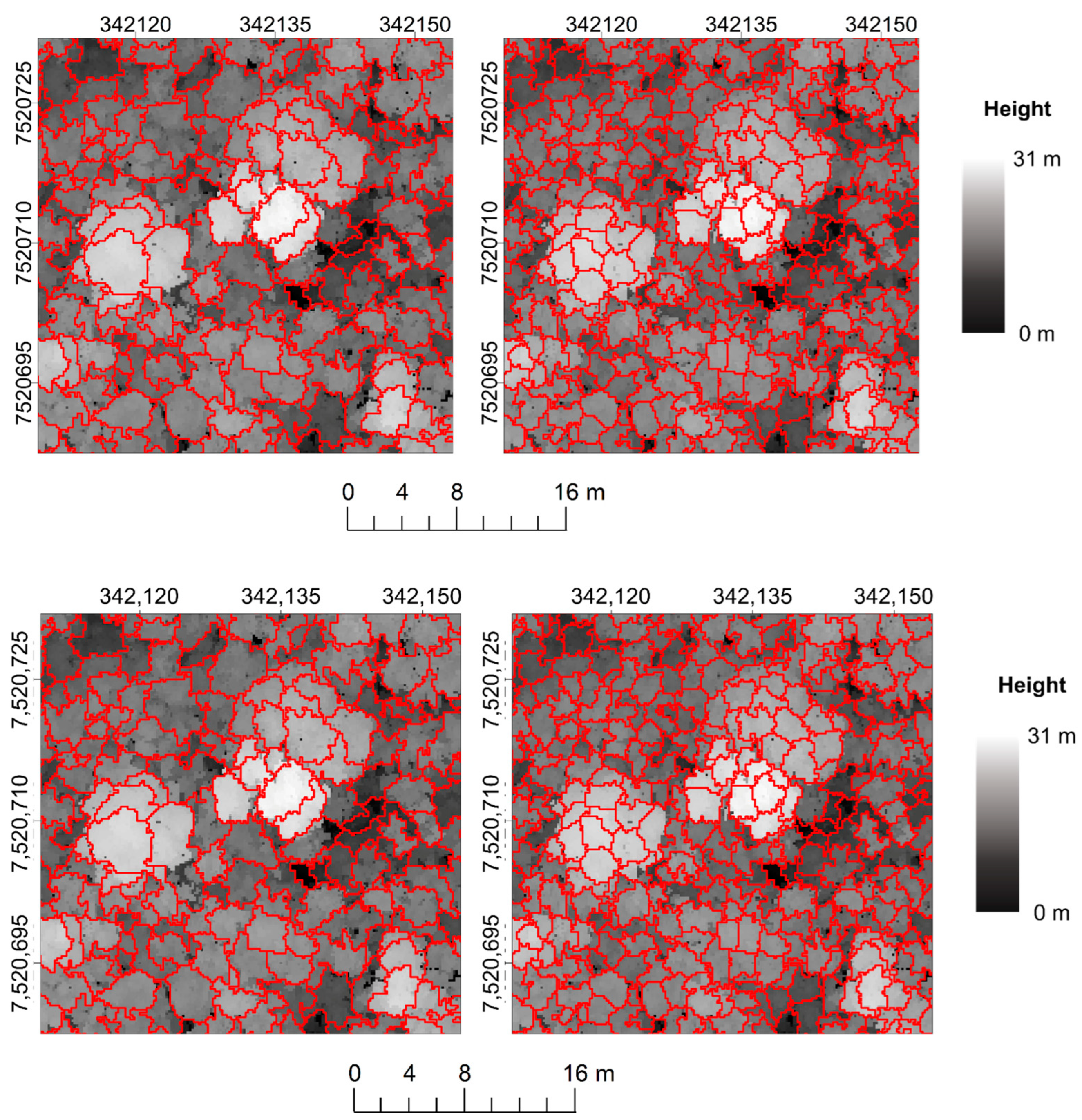
4.1. ITC Deliniation

The delineation of individual tree crowns was performed in the CHM using the superpixel method. Since the main focus of the study is to investigate which combination of hyperspectral and LiDAR metrics better classify tree species and the superpixel method leads to over-segmentation, the over-segmentation was corrected in a semi-automated way. At first, small segments created by the superpixel algorithm were merged according to the predefined criteria (Table 4). After this automatic step, the merged superpixels were checked, and the quality of the segmentation was improved using vector editing tools. This method ensured that all trees were correctly delineated, and no samples were left out. However, this worked for this study with a small sample of trees, but more robust methods of delineating tree crowns in tropical forests are needed.
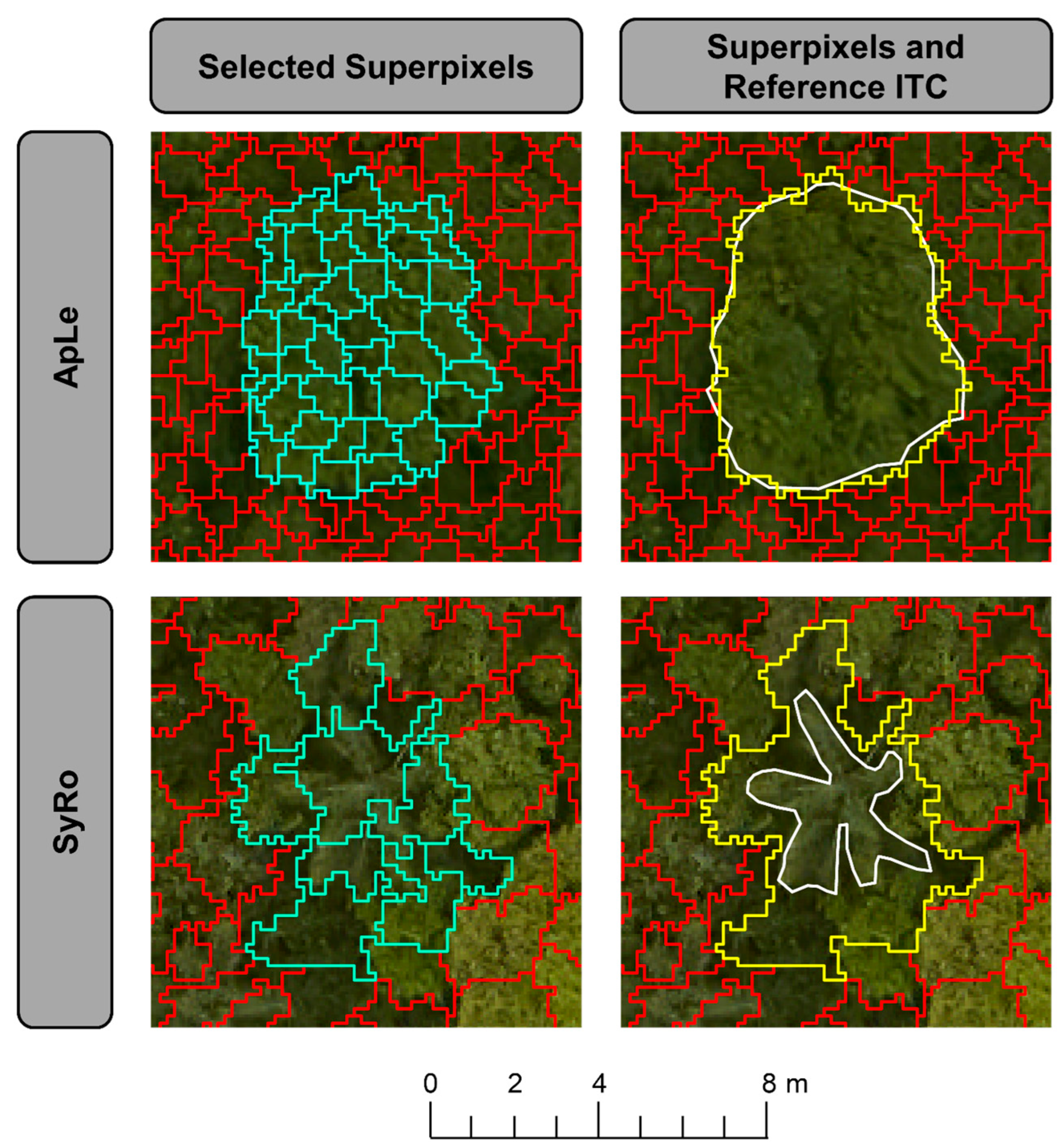
It was shown that the superpixel approach was superior to the watershed algorithm for delineating tree crowns from the CHM at Ponte Branca Forest remnant [47]. A segmentation accuracy of 62% was achieved. However, at [
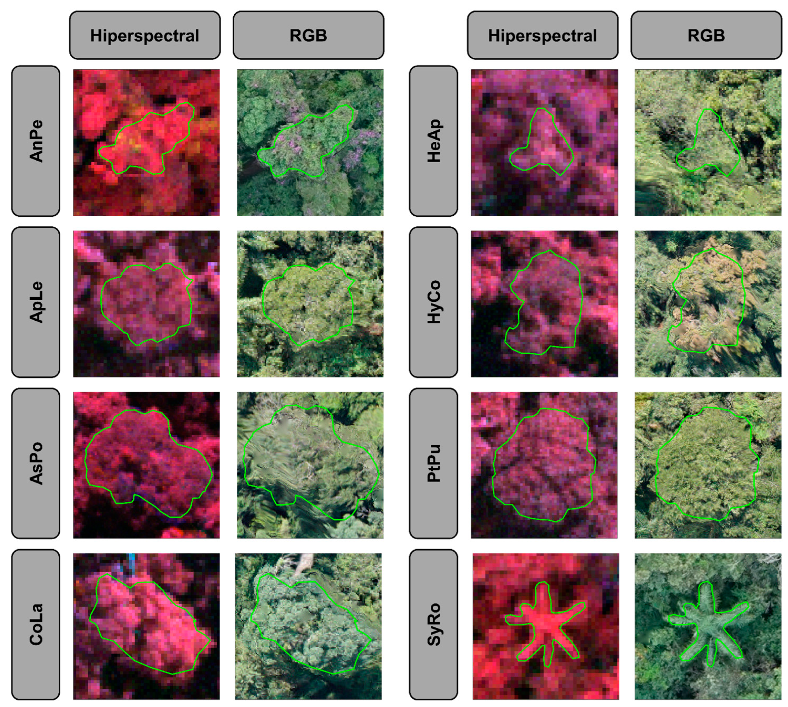
47], the presence of a SyRo palm tree whose crown is not circular was reported, making the automatic process challenging. It required smaller superpixels to distinguish palm tree crowns (star-shaped, Figure 9), but it conferred over-segmentation to the other species within the tropical forest that have wider and more circular-like shape crowns. The same problem was found in our study, and the segments referring to the SyRo palm tree species had to be manually corrected in most cases.
In Brazilian Amazon forest, ref. [103] tested some ITC delineation algorithms using the CHM from LiDAR available in lidR package for R [65]. The best result was obtained by the method developed by [104], which is based on seeds and Voronoi tessellation, with an accuracy of 65%. The authors mentioned that raster CHM-based methods are ineffective to detect trees present in lower strata.
In another inland Atlantic Forest remnant in Brazil, ref. [105] tested a new automatic method for delineating ITC using high-resolution multispectral satellite images. The method encompasses several steps, namely pre-processing, selection of forest pixels, enhancement and detection of pixels in the crown borders, correction of shade in large trees, and segmentation of the tree crowns. The accuracy of the method was 79%, showing it to be an effective method for large tree crowns; however, the method is ineffective in detecting trees in the understory and trees located in shadowed areas due to other trees or terrain shade.
All the authors cited above mention the difficulty of delineating ITCs in tropical forests due to the complexity and heterogeneity of forest formations and the difficulty of performing the segmentation of species in the lower strata, mainly because smaller trees are below the crowns of larger trees. According to [75], a perfect ITC delineation in tropical forests is unrealistic. However, partial information that allows the delineation of dominant, rare, or invasive tree species that could be important ecological indicators is of great value for better understanding these complex ecosystems.

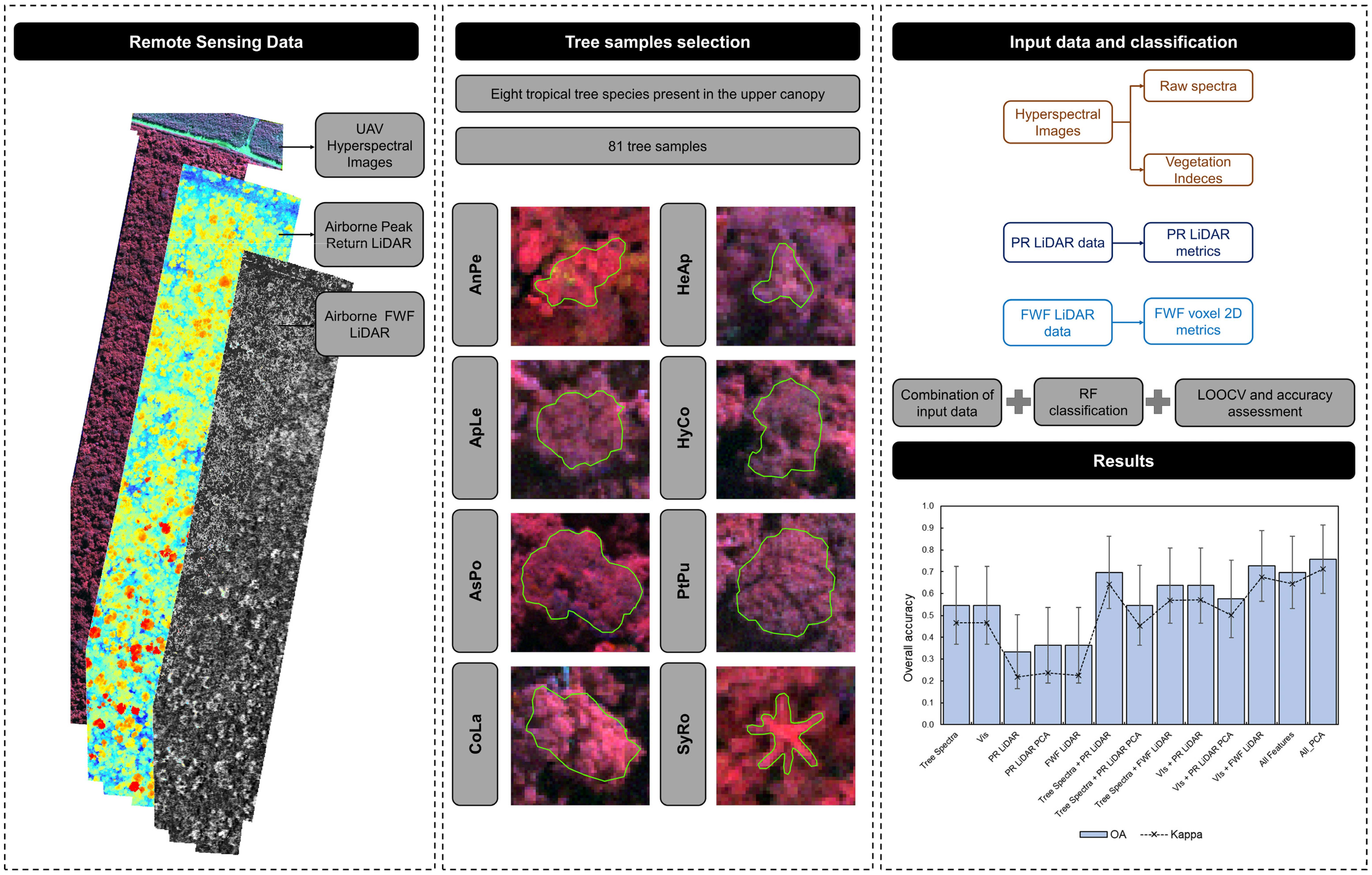
4.2. Tree Species Classification

In this study, we classified eight tree species in a Brazilian Atlantic Forest remnant using multisource remote sensing data. Three different datasets were used: hyperspectral images, PR LiDAR, and FWF LiDAR data. These data were used independently or combined to train and evaluate an RF tree species classifier. Many studies have addressed the classification of tree species in temperate and subtropical forests using spectral and/or geometric data (i.e., LiDAR) [4,6,106,107,108,109,110,111,112,113,114], but few studies have been realized to classify tree species in Brazilian tropical forests, mainly due to the difficulty in access to these areas, difficulty in obtaining a sufficient number of samples of each species, great heterogeneity, and diversity of tree species in these forests. Thus, our discussion will be based on studies with similar applications for at least tropical and subtropical forests, whenever possible.
To classify eight emerging tree species in the Ponte Branca Forest remnant (same study area), ref. [
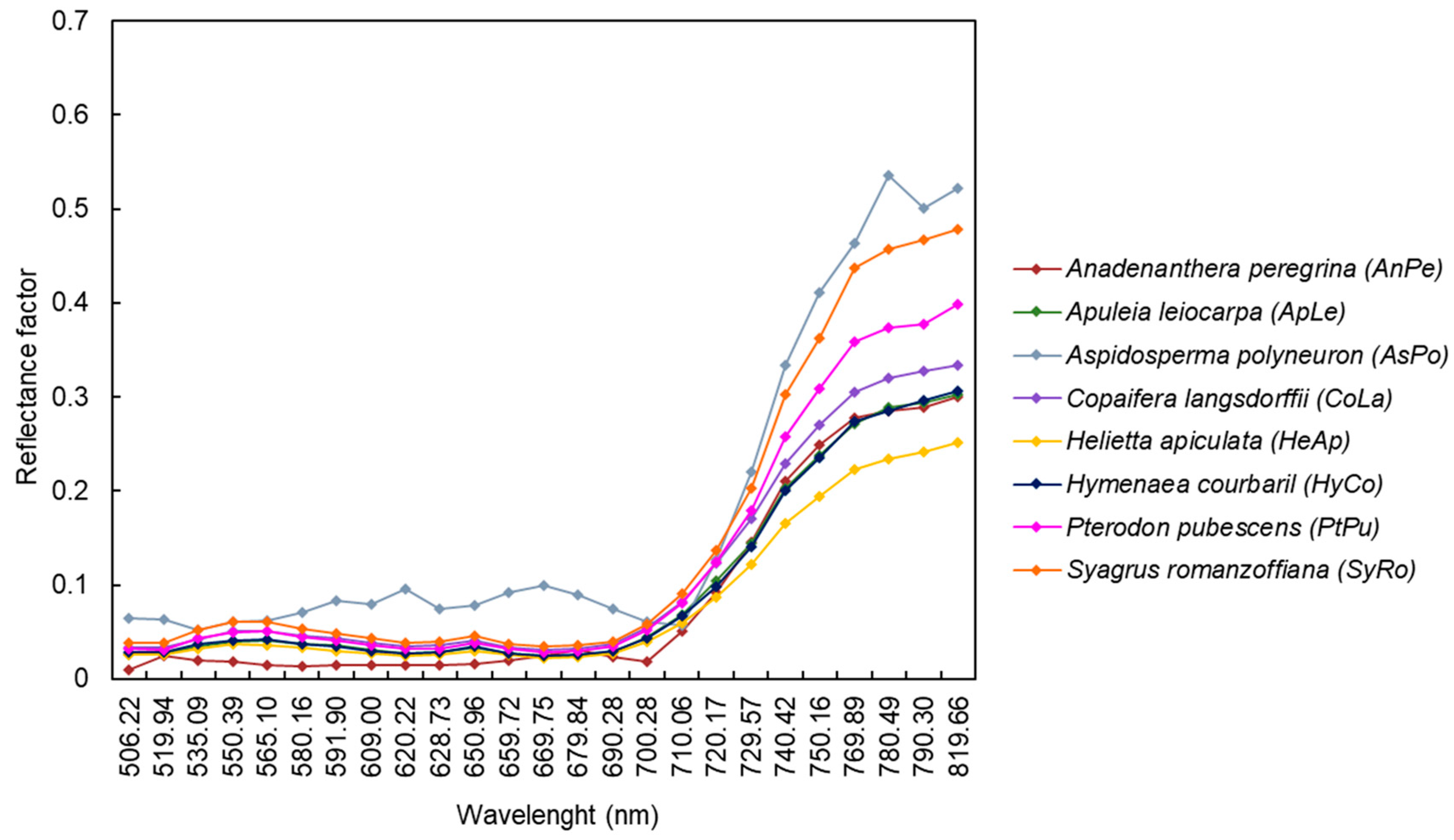
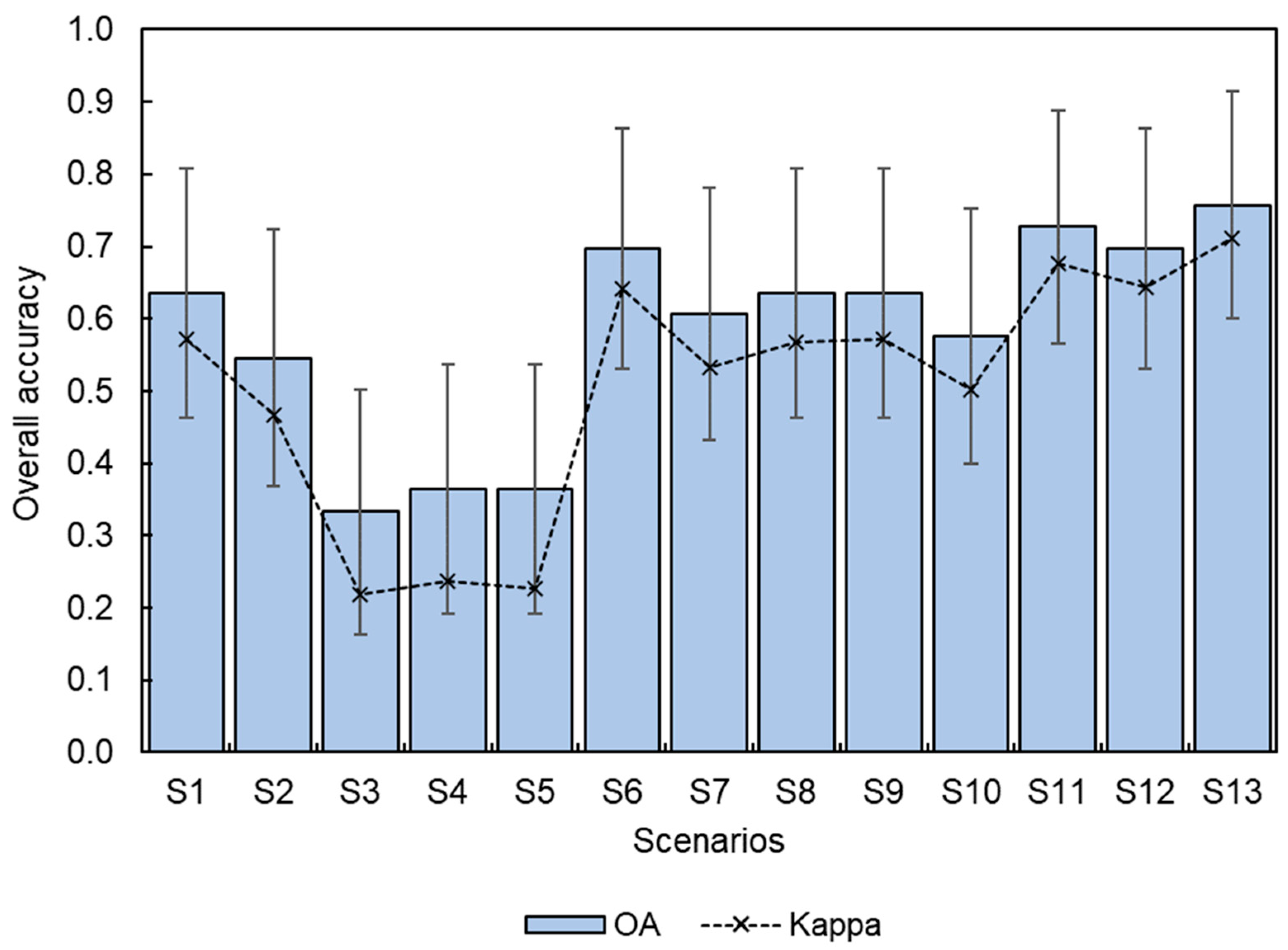
35] used hyperspectral data from Rikola camera onboard of UAV, collected on three different dates, to understand whether multitemporal data can improve the classification. The variables used were normalized and non-normalized tree species spectra. The use of temporal spectral information improved classification performance for three of the eight analysed species. However, for the other species, a difference in environmental conditions between years influenced flowering and defoliation of the species even in the same season, thus altering the spectral response, as well as the time of image acquisition. The best result was obtained with the normalized spectra (OA of 50%). In our study, the OA was similar (55%) using the raw spectra (Figure 11). The aforementioned authors reported a difference in spatial position between ITCs over the years, and some neighbouring trees interfere the spectral response of the tree species to be classified. In our case, there was no misalignment between the same ITC sample, but for the same species, there were samples on two different dates (2016 and 2017). Even though the data in different years were collected in the same season, there was a lag of one year and one month (Table 3). Thus, the same species can present different physiological and phenological behaviour in different years, which may explain why the raw spectra and VIs were not effective in differentiating tree species in the Ponte Branca Forest remnant. The most important features found by [
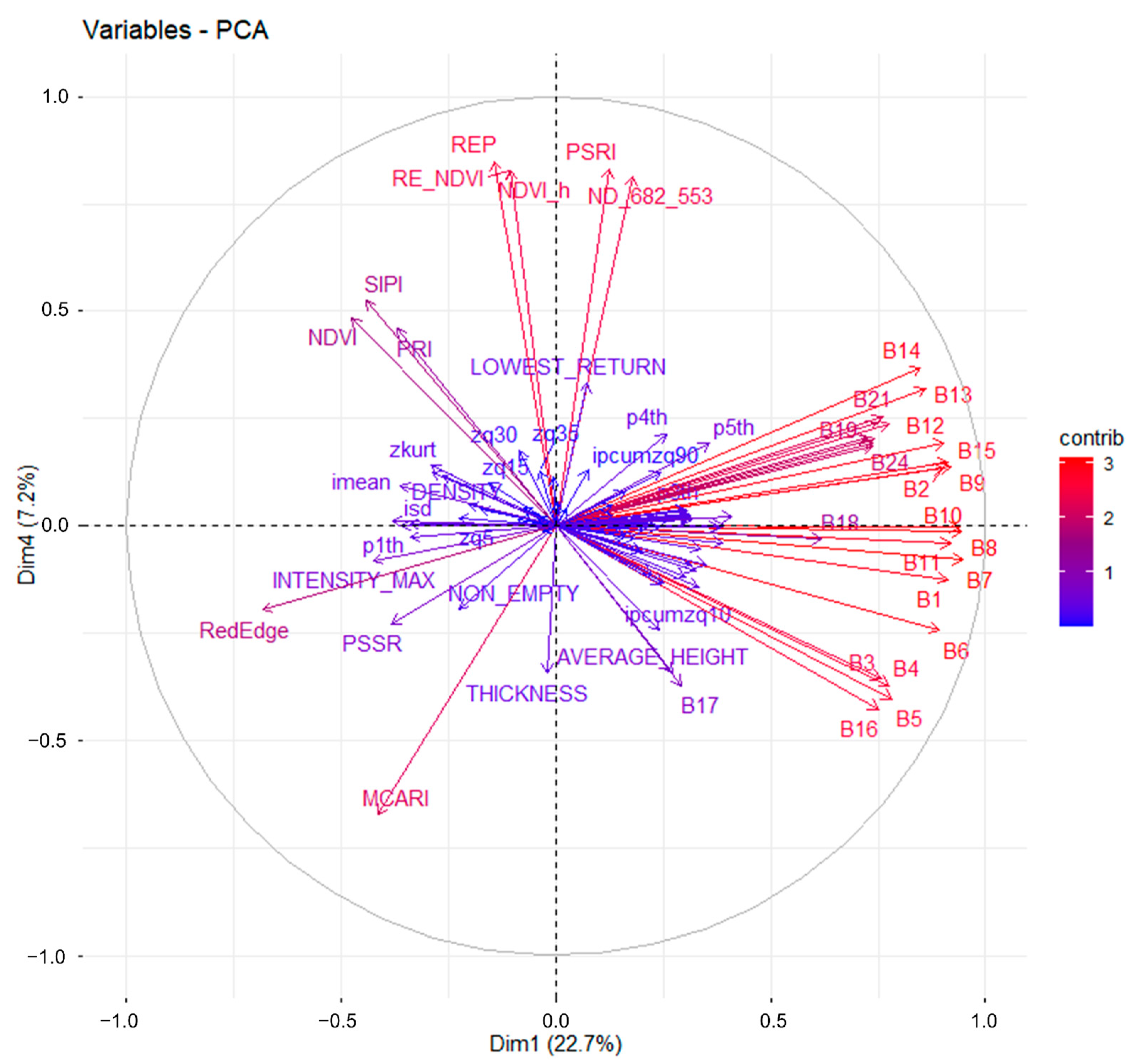
35] were the wavelengths, mainly from 628.73 nm to 780.49 nm (Band 10 to Band 23), which coincide with the bands that most contribute to the PC (Figure 14) for the best classification scenario in our study. This makes sense as band configuration of the camera used in both studies were the same, and the species chosen for classification were similar, as well.
In another inland Atlantic Forest remnant in Brazil, [
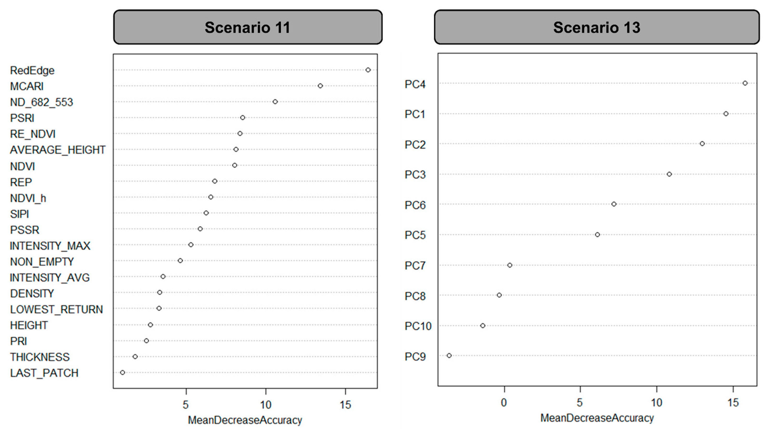
29] classified eight forest species using airborne hyperspectral images obtained with the AisaEAGLE sensor in the VNIR spectrum (visible and near-infrared) and the AisaHAWK sensor in the SWIR spectrum (shortwave-infrared). Various combinations of wavelengths and VIs were tested. Species discrimination performed best using visible bands (mainly wavelengths located at 550 nm and 650 nm) and SWIR bands. Vegetation indices contributed positively to the classification when integrated with VNIR features and should be used if the sensor does not acquire data in the SWIR wavelengths. The PSRI vegetation index (see Table 5) was one of the most important for tree species differentiation and, in our case, had the fourth highest relative importance (see Figure 13) for the second-best classification scenario (S11). The best classification accuracy obtained by [29] was 90.1%. This result was better than the result obtained by us, even for the best classification scenario (S13—OA of 76%). One of the reasons is the sample sufficiency. The forest remnant in [29] study has a larger area and a better conservation state; consequently, more trees are present in the upper canopy. A total of 273 samples of eight species were selected while in our study, only 81 samples of eight species were selected. In addition, the Rikola camera does not collect data in the SWIR spectrum.
It was possible to verify that data from narrowband sensors (i.e., hyperspectral) are an important tool in the discrimination of tropical species since it is possible to obtain specific wavelengths and vegetation indices in parts of the spectrum where it is possible to differentiate species according to the spectral response. Even the results achieved by us using only spectral information were not satisfactory; wavelengths in the VIS, Red-edge, and NIR spectrum proved to be suitable to calculate most of the VIs and for classifying different tree species until certain level in our study.
It is possible with PR LiDAR data extract information that describe the structure and geometry of forests, and this information also has the potential to discriminate tree species, but their isolated use was not effective for classification in our study. The PR LiDAR metrics and their transformation by PCA showed the lowest classification accuracy and OA (33% and 36%, respectively). Michalowska and Rapiński (2021) [6] commented that using only vertical structural features from PR LiDAR (i.e., height distribution) can decrease classification accuracy. Considering only the structure of the vegetation, it is not species-specific but more conditioned to the position on ecological succession (e.g., if the species is pioneer, secondary, or climax) or layer in the forest (e.g., understory, lower, medium, or upper stratum). Furthermore, tropical forests have multiple layers with smaller trees below the canopy, and therefore, PR LiDAR height distributions and pulse returns are ineffective for species separation in lower strata [6,47,113] when used independently as input for tree species classification. In more complex forests, the spectral differences are usually more pronounced than structural differences when used independently [110], which was confirmed in our study when analysing each of these features (hyperspectral images, PR LiDAR, and FWF LiDAR) separately.
While PR LiDAR metrics can decrease classification accuracy, the isolated use of FWF LiDAR metrics have great potential for classification of tree species, as the analysis of the complete waveform allows a better interpretation of the physical structure and geometric backscatter properties of the intercepted objects [13,17,115,116]. Some authors, such as [19,117], used metrics related to the number of waveform peaks, waveform distance, height of median energy, roughness, and return of waveform energy for tree species classification. Hollaus et al. (2009) [118] used FWF LiDAR metrics related to echo height distributions, mean and standard deviation of echo widths, mean intensities, and backscatter cross-sections. In China’s subtropical forests, the OA was 68.6% for classification of six tree species [117]. Reitberger et al. (2008) [19] found an OA of 79% for the classification of leaf-on tree species and OA of 95% for the classification of leaf-off tree species in Bavarian Forest National Park in Germany, and in pre-Alps region of Austria, three species (beech, spruce and larch) were classified with an OA of 85% by [118]. All these authors used metrics extracted from FWF LiDAR data. However, in our study, using only FWF LiDAR metrics to classify tree species was unsuccessful (OA of 36%). It is noteworthy that none of the cited studies were performed in complex tropical forests; in addition, the DASOS software provided a different set of FWF metrics that related to the spatial distribution of voxels that contain or do not contain a waveform sample. It is worth noting that these metrics relating to the voxel distribution could also be extracted using point clouds, as each waveform sample is actually a point associated with an intensity.
When used isolated, spectral data from the Rikola camera and the geometric/structural data from LiDAR were not effective for classification (S1 to S5), LiDAR geometric data, especially when combined with radiometric data, intensity, and spectral data, provided valuable information for the classification of tree species in complex forests [4,6].
It is possible to notice that the metrics related to the voxels extracted from the FWF LiDAR data using DASOS, and the VIs from the Rikola camera were one of the best combinations for the classification of the eight species of the Ponte Branca Forest remnant, with an OA of 73%., an improvement of 18% comparing the classification performed with the spectra and VIs extracted from the Rikola camera, and 36% using the FWF LiDAR metrics alone. Buddenbaum et al. (2013) [10], to classify two different forest species (Spruce and Douglas Fir) that were in different age classes, used 122 spectral bands of the HyMap hyperspectral sensor and normalized intensities of the waveforms that intercepted voxel columns with dimensions of 0.5 m. Combining these two data sources, the OA was 72.2%, improving classification accuracy by 16% when compared to using spectral bands only and 5.5% when using spectral bands and percentile heights of PR LiDAR data that was isolated. The FWF LiDAR metric related to the intensity of the voxels intercepted by the waveform samples proved to be an important metric in the differentiation of forest species, including in our study, in which it was important both for S11 and for S13 (Figure 13). Liao et al. (2018) [22] also confirmed an improvement in the accuracy of the classification of seven forest species in the western part of Belgium using different height percentiles of FWF LiDAR with hyperspectral images. The improvement was 7.7% compared to the classification using only hyperspectral bands and 24.8% compared to using only raster LiDAR FWF. It is worth mentioning that the metrics related to height percentiles are dependent on the point cloud density, which makes it difficult to compare with other study areas or different acquisition parameters of the point cloud. Thus, a benchmarking data to test algorithms across different acquisitions and study areas is necessary for understanding how the tree species classification performs using different types of LiDAR metrics [119]. The DASOS software normalizes the data during voxelization and deals with the irregular scan pattern, and the extracted metrics are not dependent on the point density [72].
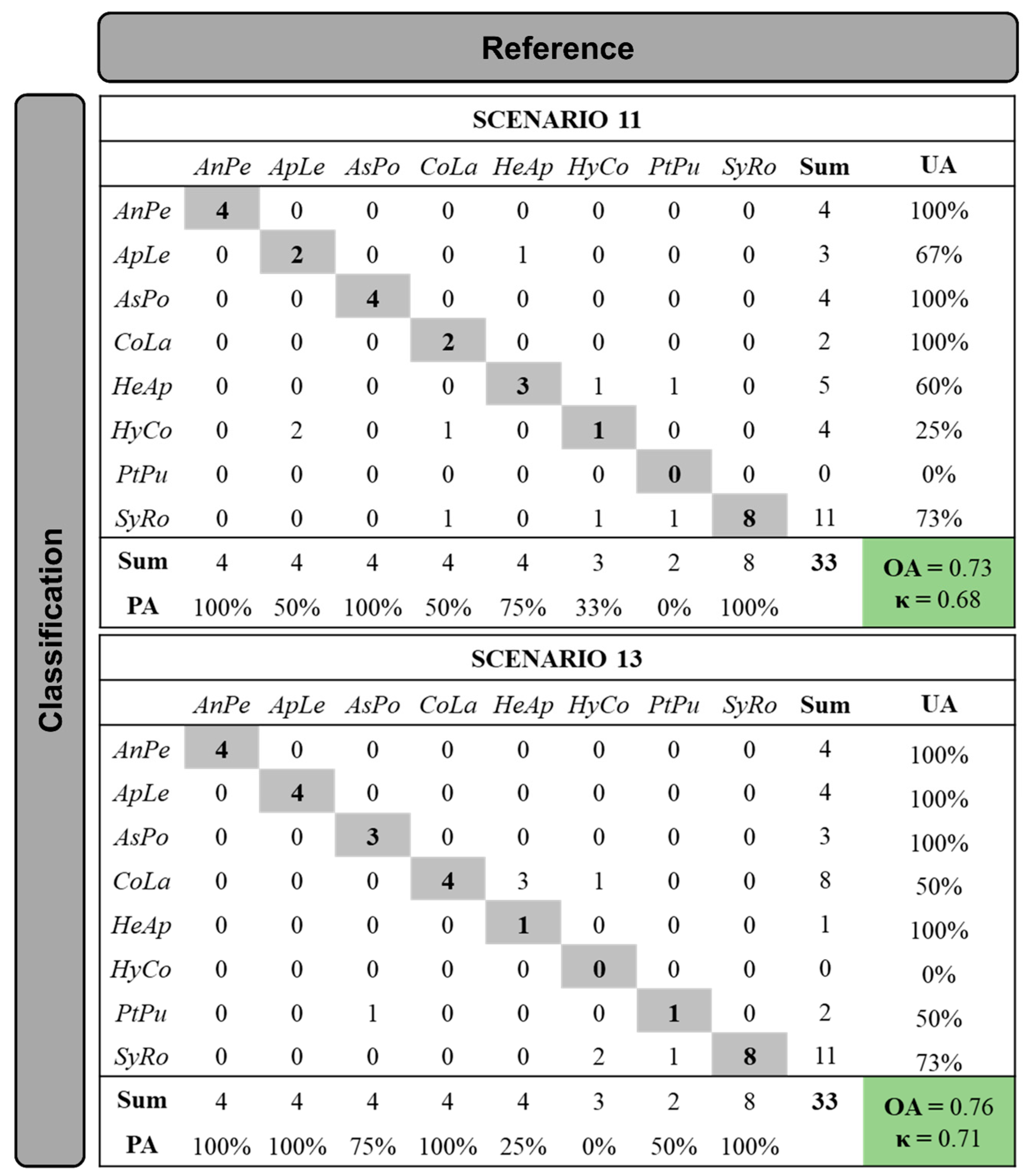
Although the FWF LiDAR metrics performed better when combined with the VIs in classifying tree species, the difference was small when we looked at the confidence intervals (Figure 11) for the scenarios that combine both PR LiDAR and FWF LiDAR metrics with the information spectra and VIs (S8–S9 and S11 to S13). S13 includes all the metrics included in S11, and a small increase in classification accuracy was observed from including the extra metrics extracted from the PR data and the spectral data except for the scenarios, whose combinations were made with the PR LiDAR metrics transformed by PCA (S7 and S10).
As FWF LiDAR data require more computer memory than PR LiDAR data, the data processing is more time consuming and requires more computational effort, and few tools are available for processing and extracting information from FWF LiDAR point clouds [72,120]. In addition, due to the advancement of LiDAR systems, it is possible to obtain several returns for each emitted pulse. Thus, PR LiDAR metrics can be effective for tree species classification when FWF LiDAR data are not available and/or it is not possible to process them.
There are many tools and workflows for processing PR LiDAR point clouds, and several authors have already proven that the combined use of LiDAR metrics and spectral information from hyperspectral sensors (e.g., raw spectrum and VIs) improve the classification of tree species in different types of forest. Asner et al. (2008) [121], for the classification of invasive tree species in Hawaiian tropical forests, found an improvement in accuracy from 63% to 91% using tree species spectra and LiDAR heights. Shen and Cao et al. (2017) [122] found an improvement of approximately 6% in the classification of five species, and ref. [110] found an increase in classification accuracy of 18 tree species of approximately 7% using both VIs and LiDAR metrics in Chinese subtropical forests. In our study area, improvements were 15% when combining raw spectra with LiDAR PR metrics and 9% when combining VIs with LiDAR PR metrics in classifying eight tree species. This corroborates the potential that the combination of hyperspectral and geometric data from LiDAR, mainly related to height percentiles and percentage of returns, have to improve the accuracy of tree species classifications, including in tropical forests.
Using all features extracted from different data sources for classification (i.e. spectra and VIs from images of the camera Rikola, PR, and FWF LiDAR metrics), we achieved a classification OA of 70% (Scenario 12), and transforming all features by PCA, the OA was 76% (Scenario 13), the best result obtained in this study. Using a large set of features as input data for classification, ref. [110] combined VIs and PCA from hyperspectral images, textural information from RGB images, and structural metrics from LiDAR, totalling 64 features for the classification of tree species in Chinese subtropical forests. The OA was 91.8%, a better result than just using the isolated features or combining them two by two (e.g., LiDAR and VIs). For the classification of 12 tree species in a Brazilian subtropical forest, ref. [79] tested several scenarios with different inputs, and one of the scenarios contained 68 features (e.g., raw spectra and VIs obtained from hyperspectral images, photogrammetric point cloud metrics, CHM, and textural information). The OA was 70.7% with a difference of less than 2% obtained for the best scenario that used raw spectra, VIs, and structural information from the photogrammetric point cloud as input.
When using many features as input data for classification with the RF algorithm, the features are randomly selected at each node of the tree [123]. If any feature that does not contribute to species differentiation is selected, the classification performance may decline [123]. The more features that do not contribute to the separation of tree species are added in the RF algorithm, the greater the probability of these features being selected at each node, increasing the algorithm generalization error in addition to generating very large trees [123,124]. Thus, a pre-selection of features that have the greatest potential to differentiate species can optimize and improve classification accuracy. However, as trees are complex structures, different features from different data sources (i.e., different remote sensors) can be complementary to improve the separability and classification of tree species. This can be seen in the results obtained in this study, as well as in other studies cited above, in which the use of many features did not decrease accuracy, but rather, it was similar to or even improved the classification accuracy when compared with a pre-selection or use of fewer features as input data for classifying tree species.
The transformation of the PR LiDAR metrics by the PCA and the use of these isolated features with the spectra or with the VIs were not very effective in the classification. However, when using all the features extracted from the hyperspectral images and the PR and FWF LiDAR point clouds transformed by the PCA, it resulted in the best classification accuracy (OA of 76%). According to [22], the high dimensionality and redundancy when using hyperspectral data mainly makes it difficult to extract information from moving windows in raster data. Thus, the transformation by PCA facilitates the extraction of information using moving windows. In addition to decreasing the correlation between features that may be redundant, the PCA transformation can improve the classification accuracy when using small training set sizes [125].

5. Conclusions

In this study, we tested the automatic classification of eight tree species present in the upper canopy of a remnant of the Brazilian Atlantic Forest. Thirteen different classification scenarios were tested using remote sensing data from different sources (i.e., hyperspectral images collected from a UAV and airborne PR (peak return) and FWF (full-waveform LiDAR) as input data for the classification.
The segmentation of tree crowns was performed using the superpixels algorithm. Due to the low number of samples (81 trees), a manual correction of the segments that were not correctly delineated was made. Despite being effective, the method is time consuming, especially when working with a large number of samples, and it is recommended to have more studies on this topic for tropical forests.
Among the tested scenarios, the isolated use of LiDAR metrics for classification regardless of the type of return and the transformation by PCA (principal component analysis), was not effective for the classification, resulting in the lowest overall accuracy (between 33% and 36%). The use of the raw spectra of the hyperspectral images and the VIs (vegetation indices) had a better accuracy than the use of LiDAR data (55% for both features). However, the results with this data configuration were still not satisfactory.
When spectral features were combined with LiDAR metrics, there was a considerable increase in classification accuracy, between 64% and 76%, except when using the combination of raw spectra or VIs with PR LiDAR metrics, transformed by PCA (accuracy of 55% and 58%, respectively). The use of all features (raw spectra, VIs, PR, and FWF LiDAR), transformed by PCA, was the best classification scenario (overall accuracy of 76%), followed by the use of VIs and FWF LiDAR metrics (overall accuracy of 73%). However, considering the confidence intervals were at 95% probability, there was no significant difference between the scenarios using PR or FWF LiDAR metrics with the raw spectra or VIs.
Analysing the results of the overall accuracies obtained in the different classification scenarios analysed and the most important features for the best scenarios provided by the RF (random forest) algorithm, it can be concluded that cameras that collect data in visible, Red-edge, and NIR wavelengths are sufficient to calculate most of the VIs providing sufficient spectral information. Combined with PR LiDAR metrics (e.g., height percentiles and number of returns for each emitted pulse), they can achieve satisfactory accuracies in the classification of tree species in complex forests.
Data acquisition with UAVs can reduce costs and improve usability, but it requires the development of suitable sensors, such as lightweight multispectral cameras and LiDAR with the ability to record multiple returns, intensity, and with a greater density of points. Because UAVs can operate at a lower flight height, they allow greater flexibility for data collection in different areas and can generate outputs with good accuracy.
Despite the difficulties observed in this study, mainly in relation to the low sampling sufficiency of the trees, the time lag between the different flight campaigns, and the high heterogeneity of the forest canopy, the results of the classification were satisfactory for the complex forest environment studied. These results can serve for management and conservation practices of these forest remnants, allowing for a better understanding of the spatial distribution of species with a potential for forest restoration.

Supplementary Materials

The following supporting information can be downloaded at: https://www.mdpi.com/article/10.3390/f14050945/s1, Figure S1: Spectra obtained from each tree for each species, from hyperspectral orthomosaics. Figure S2: Distribution of species classified in the best scenario (S13). The segment colour represents the classification result, and the border colour refers to the correct field identification.

Author Contributions

Conceptualization, R.P.M.-N., A.M.G.T., N.N.I., E.H., E.A.S.M., M.M. and H.C.D.; methodology, R.P.M.-N., A.M.G.T., N.N.I., E.H. and E.A.S.M.; software, R.P.M.-N., E.H., E.A.S.M. and M.M.; validation, R.P.M.-N. and H.C.D.; formal analysis, R.P.M.-N.; investigation, R.P.M.-N., A.M.G.T., N.N.I., E.H. and M.M.; resources, A.M.G.T., N.N.I. and E.H.; data curation, R.P.M.-N.; writing—original draft preparation, R.P.M.-N.; writing—review and editing, R R.P.M.-N., A.M.G.T., N.N.I., E.H., E.A.S.M., M.M. and H.C.D.; visualization, R.P.M.-N., A.M.G.T., N.N.I. and H.C.D.; supervision, A.M.G.T., N.N.I., M.M. and H.C.D.; project administration, A.M.G.T., N.N.I. and E.H.; funding acquisition, A.M.G.T., N.N.I. and E.H. All authors have read and agreed to the published version of the manuscript.

Funding

This study was funded by the Coordenação de Aperfeiçoamento de Pessoal de Nível Superior–Brazil (CAPES)–Finance Code 001 (process number 88882.433953/2019-01); by the Programa Institucional de Internacionalização (CAPES/PrInt)–process number 88881.310314/2018-01; by the Conselho Nacional de Desenvolvimento Científico e Tecnológico–Brazil (CNPq)–process numbers 404379/2016-8 and 303670/2018-5; and by the Brazilian–Finnish joint project “Unmanned Airborne Vehicle–Based 4D Remote Sensing for Mapping Rain Forest Biodiversity and its Change in Brazil”, financed part by São Paulo Research Foundation (FAPESP), grant number 2013/50426-4 and part by Academy of Finland (AKA), grant number 273806.

Data Availability Statement

The data presented in this study are not available on request. The data are not publicly available due to as the study area is protected by federal laws.

Acknowledgments

The authors would like to thank Baltazar Casagrande and Valter Ribeiro Campos for their assistance with the field surveys and species recognition and the company ENGEMAP for providing the ALS point cloud from the study area. M.M. was funded by a UKRI Future Leaders Fellowship (MR/T019832/1). For the purpose of open access, the author has applied a Creative Commons Attribution (CC BY) licence to any Author Accepted Manuscript version arising.

Conflicts of Interest

The authors declare no conflict of interest.

References

  1. Zhou, X.; Fu, Y.; Zhou, L.; Li, B.; Luo, Y. An Imperative Need for Global Change Research in Tropical Forests. Tree Physiol. 2013, 33, 903–912. [Google Scholar] [CrossRef] [PubMed]
  2. Hassan, R.; Scholes, R.; Ash, N. Ecosystems and Human Well-Being: Current State and Trends; Island Press: Washington, DC, USA, 2005. [Google Scholar]
  3. Lopez-Gonzalez, G.; Lewis, S.L.; Burkitt, M.; Phillips, O.L. ForestPlots. Net: A Web Application and Research Tool to Manage and Analyse Tropical Forest Plot Data. J. Veg. Sci. 2011, 22, 610–613. [Google Scholar] [CrossRef]
  4. Fassnacht, F.E.; Latifi, H.; Stereńczak, K.; Modzelewska, A.; Lefsky, M.; Waser, L.T.; Straub, C.; Ghosh, A. Review of Studies on Tree Species Classification from Remotely Sensed Data. Remote Sens. Environ. 2016, 186, 64–87. [Google Scholar] [CrossRef]
  5. Piiroinen, R.; Heiskanen, J.; Maeda, E.; Viinikka, A.; Pellikka, P. Classification of Tree Species in a Diverse African Agroforestry Landscape Using Imaging Spectroscopy and Laser Scanning. Remote Sens. 2017, 9, 875. [Google Scholar] [CrossRef]
  6. Michalowska, M.; Rapiński, J. A Review of Tree Species Classification Based on Airborne LiDAR Data and Applied Classifiers. Remote Sens. 2021, 13, 353. [Google Scholar] [CrossRef]
  7. Cochrane, M.A. Using Vegetation Reflectance Variability for Species Level Classification of Hyperspectral Data. Int. J. Remote Sens. 2000, 21, 2075–2087. [Google Scholar] [CrossRef]
  8. Féret, J.-B.; Asner, G.P. Tree Species Discrimination in Tropical Forests Using Airborne Imaging Spectroscopy. IEEE Trans. Geosci. Remote Sens. 2012, 51, 73–84. [Google Scholar] [CrossRef]
  9. Zhang, J.; Rivard, B.; Sánchez-Azofeifa, A.; Castro-Esau, K. Intra-and Inter-Class Spectral Variability of Tropical Tree Species at La Selva, Costa Rica: Implications for Species Identification Using HYDICE Imagery. Remote Sens. Environ. 2006, 105, 129–141. [Google Scholar] [CrossRef]
  10. Buddenbaum, H.; Seeling, S.; Hill, J. Fusion of Full-Waveform Lidar and Imaging Spectroscopy Remote Sensing Data for the Characterization of Forest Stands. Int. J. Remote Sens. 2013, 34, 4511–4524. [Google Scholar] [CrossRef]
  11. Kim, S.; McGaughey, R.J.; Andersen, H.-E.; Schreuder, G. Tree Species Differentiation Using Intensity Data Derived from Leaf-on and Leaf-off Airborne Laser Scanner Data. Remote Sens. Environ. 2009, 113, 1575–1586. [Google Scholar] [CrossRef]
  12. Morsdorf, F.; Mårell, A.; Koetz, B.; Cassagne, N.; Pimont, F.; Rigolot, E.; Allgöwer, B. Discrimination of Vegetation Strata in a Multi-Layered Mediterranean Forest Ecosystem Using Height and Intensity Information Derived from Airborne Laser Scanning. Remote Sens. Environ. 2010, 114, 1403–1415. [Google Scholar] [CrossRef]
  13. Shan, J.; Toth, C.K. Topographic Laser Ranging and Scanning: Principles and Processing; CRC Press: New York, NY, USA, 2018. [Google Scholar]
  14. Favorskaya, M.N.; Jain, L.C. Overview of LiDAR Technologies and Equipment for Land Cover Scanning. In Handbook on Advances in Remote Sensing and Geographic Information Systems; Springer: Berlin/Heidelberg, Germany, 2017; Volume 122, pp. 19–68. [Google Scholar]
  15. Thiel, K.H.; Wehr, A. Performance Capabilities of Laser Scanners–an Overview and Measurement Principle Analysis. Int. Arch. Photogramm. Remote Sens. Spat. Inf. Sci. 2004, 36, 14–18. [Google Scholar]
  16. Lim, K.; Treitz, P.; Wulder, M.; St-Onge, B.; Flood, M. LiDAR Remote Sensing of Forest Structure. Prog. Phys. Geogr. 2003, 27, 88–106. [Google Scholar] [CrossRef]
  17. Mallet, C.; Bretar, F. Full-Waveform Topographic Lidar: State-of-the-Art. ISPRS J. Photogramm. Remote Sens. 2009, 64, 1–16. [Google Scholar] [CrossRef]
  18. Pirotti, F. Analysis of Full-Waveform LiDAR Data for Forestry Applications: A Review of Investigations and Methods. Iforest-Biogeosciences For. 2011, 4, 100. [Google Scholar] [CrossRef]
  19. Reitberger, J.; Krzystek, P.; Stilla, U. Analysis of Full Waveform LIDAR Data for the Classification of Deciduous and Coniferous Trees. Int. J. Remote Sens. 2008, 29, 1407–1431. [Google Scholar] [CrossRef]
  20. RIEGL DataSheet LMS-Q680i. Available online: http://www.riegl.com/uploads/tx_pxpriegldownloads/10_DataSheet_LMS-Q680i_28-09-2012_01.pdf (accessed on 7 April 2021).
  21. Luo, S.; Wang, C.; Xi, X.; Zeng, H.; Li, D.; Xia, S.; Wang, P. Fusion of Airborne Discrete-Return LiDAR and Hyperspectral Data for Land Cover Classification. Remote Sens. 2016, 8, 3. [Google Scholar] [CrossRef]
  22. Liao, W.; Van Coillie, F.; Gao, L.; Li, L.; Zhang, B.; Chanussot, J. Deep Learning for Fusion of APEX Hyperspectral and Full-Waveform LiDAR Remote Sensing Data for Tree Species Mapping. IEEE Access 2018, 6, 68716–68729. [Google Scholar] [CrossRef]
  23. Guerra, T.N.F.; Rodal, M.J.N.; e Silva, A.C.B.L.; Alves, M.; Silva, M.A.M.; de Araújo Mendes, P.G. Influence of Edge and Topography on the Vegetation in an Atlantic Forest Remnant in Northeastern Brazil. J. For. Res. 2013, 18, 200–208. [Google Scholar] [CrossRef]
  24. Scarano, F.R.; Ceotto, P. Brazilian Atlantic Forest: Impact, Vulnerability, and Adaptation to Climate Change. Biodivers. Conserv. 2015, 24, 2319–2331. [Google Scholar] [CrossRef]
  25. Haddad, N.M.; Brudvig, L.A.; Clobert, J.; Davies, K.F.; Gonzalez, A.; Holt, R.D.; Lovejoy, T.E.; Sexton, J.O.; Austin, M.P.; Collins, C.D. Habitat Fragmentation and Its Lasting Impact on Earth’s Ecosystems. Sci. Adv. 2015, 1, e1500052. [Google Scholar] [CrossRef]
  26. Rodrigues, R.R.; Lima, R.A.; Gandolfi, S.; Nave, A.G. On the Restoration of High Diversity Forests: 30 Years of Experience in the Brazilian Atlantic Forest. Biol. Conserv. 2009, 142, 1242–1251. [Google Scholar] [CrossRef]
  27. Werneck, M.d.S.; Sobral, M.E.G.; Rocha, C.T.V.; Landau, E.C.; Stehmann, J.R. Distribution and Endemism of Angiosperms in the Atlantic Forest. Nat. Conserv. 2011, 9, 188–193. [Google Scholar] [CrossRef]
  28. Myers, N.; Mittermeier, R.A.; Mittermeier, C.G.; Da Fonseca, G.A.; Kent, J. Biodiversity Hotspots for Conservation Priorities. Nature 2000, 403, 853. [Google Scholar] [CrossRef] [PubMed]
  29. Ferreira, M.P.; Zortea, M.; Zanotta, D.C.; Shimabukuro, Y.E.; de Souza Filho, C.R. Mapping Tree Species in Tropical Seasonal Semi-Deciduous Forests with Hyperspectral and Multispectral Data. Remote Sens. Environ. 2016, 179, 66–78. [Google Scholar] [CrossRef]
  30. Berveglieri, A.; Imai, N.N.; Tommaselli, A.M.; Martins-Neto, R.P.; Miyoshi, G.T.; Honkavaara, E. Forest Cover Change Analysis Based on Temporal Gradients of the Vertical Structure and Density. Ecol. Indic. 2021, 126, 107597. [Google Scholar] [CrossRef]
  31. Berveglieri, A.; Imai, N.N.; Tommaselli, A.M.; Casagrande, B.; Honkavaara, E. Successional Stages and Their Evolution in Tropical Forests Using Multi-Temporal Photogrammetric Surface Models and Superpixels. ISPRS J. Photogramm. Remote Sens. 2018, 146, 548–558. [Google Scholar] [CrossRef]
  32. Berveglieri, A.; Tommaselli, A.M.G.; Imai, N.N.; Ribeiro, E.A.W.; Guimaraes, R.B.; Honkavaara, E. Identification of Successional Stages and Cover Changes of Tropical Forest Based on Digital Surface Model Analysis. IEEE J. Sel. Top. Appl. Earth Obs. Remote Sens. 2016, 9, 5385–5397. [Google Scholar] [CrossRef]
  33. Martins-Neto, R.; Tommaselli, A.; Imai, N.; Berveglieri, A.; Thomaz, M.; Miyoshi, G.; Casagrande, B.; Guimarães, R.; Ribeiro, E.; Honkavaara, E. Structure and Tree Diversity of an Inland Atlantic Forest—A Case Study of Ponte Branca Forest Remnant, Brazil. Indones. J. Geogr. 2022, 54, 9. [Google Scholar] [CrossRef]
  34. Chase, M.W.; Christenhusz, M.J.M.; Fay, M.F.; Byng, J.W.; Judd, W.S.; Soltis, D.E.; Mabberley, D.J.; Sennikov, A.N.; Soltis, P.S.; Stevens, P.F. An Update of the Angiosperm Phylogeny Group Classification for the Orders and Families of Flowering Plants: APG IV. Bot. J. Linn. Soc. 2016, 181, 1–20. [Google Scholar] [CrossRef]
  35. Miyoshi, G.T.; Imai, N.N.; Garcia Tommaselli, A.M.; Antunes de Moraes, M.V.; Honkavaara, E. Evaluation of Hyperspectral Multitemporal Information to Improve Tree Species Identification in the Highly Diverse Atlantic Forest. Remote Sens. 2020, 12, 244. [Google Scholar] [CrossRef]
  36. Mariscal-Flores, E.J. Potencial Produtivo e Alternativas de Manejo Sustentável de Um Fragmento de Mata Atlântica Secundária, Município de Viçosa, Minas Gerais. Master’s Thesis, Universidade Federal de Viçosa, Viçosa, MG, Brazil, 1993. [Google Scholar]
  37. Souza, D.R.d.; Souza, A.L.d.; Gama, J.R.V.; Leite, H.G. Emprego de Análise Multivariada Para Estratificação Vertical de Florestas Ineqüiâneas. Rev. Árvore 2003, 27, 59–63. [Google Scholar] [CrossRef]
  38. Ishii, H.T.; Tanabe, S.; Hiura, T. Exploring the Relationships among Canopy Structure, Stand Productivity, and Biodiversity of Temperate Forest Ecosystems. For. Sci. 2004, 50, 342–355. [Google Scholar]
  39. Lesica, P.; Allendorf, F.W. Ecological Genetics and the Restoration of Plant Communities: Mix or Match? Restor. Ecol. 1999, 7, 42–50. [Google Scholar] [CrossRef]
  40. Carvalho, P.E.R. Espécies Arbóreas Brasileiras; Embrapa Informação Tecnológica Brasília: Brasília, Brazil, 2003; Volume 1. [Google Scholar]
  41. Carvalho, P.E.R. Espécies Arbóreas Brasileiras; Embrapa Informação Tecnológica Brasília: Brasília, Brazil, 2008; Volume 3. [Google Scholar]
  42. Carvalho, P.E.R. Espécies Arbóreas Brasileiras; Embrapa Informação Tecnológica Brasília: Brasília, Brazil, 2014; Volume 5. [Google Scholar]
  43. Carvalho, P.E.R. Espécies Arbóreas Brasileiras; Embrapa Informação Tecnológica Brasília: Brasília, Brazil, 2006; Volume 2. [Google Scholar]
  44. Miyoshi, G.T.; Imai, N.N.; Tommaselli, A.M.G.; Honkavaara, E.; Näsi, R.; Moriya, É.A.S. Radiometric Block Adjustment of Hyperspectral Image Blocks in the Brazilian Environment. Int. J. Remote Sens. 2018, 39, 4910–4930. [Google Scholar] [CrossRef]
  45. Oliveira, R.A.; Tommaselli, A.M.; Honkavaara, E. Geometric Calibration of a Hyperspectral Frame Camera. Photogramm. Rec. 2016, 31, 325–347. [Google Scholar] [CrossRef]
  46. Oliveira, R.A.; Tommaselli, A.M.; Honkavaara, E. Generating a Hyperspectral Digital Surface Model Using a Hyperspectral 2D Frame Camera. ISPRS J. Photogramm. Remote Sens. 2019, 147, 345–360. [Google Scholar] [CrossRef]
  47. Miyoshi, G.T. Emergent Tree Species Identification in Highly Diverse Brazilian Atlantic Forest Using Hyperspectral Images Acquired with UAV. Doctoral Thesis, Universidade Estadual Paulista, Faculdade de Ciências e Tecnologia, Presidente Prudente, SP, Brazil, 2020. [Google Scholar]
  48. Honkavaara, E.; Saari, H.; Kaivosoja, J.; Pölönen, I.; Hakala, T.; Litkey, P.; Mäkynen, J.; Pesonen, L. Processing and Assessment of Spectrometric, Stereoscopic Imagery Collected Using a Lightweight UAV Spectral Camera for Precision Agriculture. Remote Sens. 2013, 5, 5006–5039. [Google Scholar] [CrossRef]
  49. Mäkeläinen, A.; Saari, H.; Hippi, I.; Sarkeala, J.; Soukkamäki, J. 2D Hyperspectral Frame Imager Camera Data in Photogrammetric Mosaicking. ISPRS-Int. Arch. Photogramm. Remote Sens. Spat. Inf. Sci. 2013, XL-1/W2, 263–267. [Google Scholar] [CrossRef]
  50. Saari, H.; Aallos, V.-V.; Akujärvi, A.; Antila, T.; Holmlund, C.; Kantojärvi, U.; Mäkynen, J.; Ollila, J. Novel Miniaturized Hyperspectral Sensor for UAV and Space Applications. In Proceedings of the Sensors, Systems, and Next-Generation Satellites XIII; International Society for Optics and Photonics (SPIE): Bellingham, WA, USA, 2009; Volume 7474, p. 74741M. [Google Scholar]
  51. Näsi, R.; Honkavaara, E.; Lyytikäinen-Saarenmaa, P.; Blomqvist, M.; Litkey, P.; Hakala, T.; Viljanen, N.; Kantola, T.; Tanhuapää, T.; Holopainen, M. Using UAV-Based Photogrammetry and Hyperspectral Imaging for Mapping Bark Beetle Damage at Tree-Level. Remote Sens. 2015, 7, 15467–15493. [Google Scholar] [CrossRef]
  52. ASD FieldSpec® UV/VNIR. HandHeld Spectroradiometer—User’s Guide; Analytical Spectral Devices, Inc.: Boulder, CO, USA, 2002. [Google Scholar]
  53. Moriya, E.A.S.; Imai, N.N.; Tommaselli, A.M.G.; Miyoshi, G.T. Mapping Mosaic Virus in Sugarcane Based on Hyperspectral Images. IEEE J. Sel. Top. Appl. Earth Obs. Remote Sens. 2017, 10, 740–748. [Google Scholar] [CrossRef]
  54. Honkavaara, E.; Kaivosoja, J.; Mäkynen, J.; Pellikka, I.; Pesonen, L.; Saari, H.; Salo, H.; Hakala, T.; Marklelin, L.; Rosnell, T. Hyperspectral Reflectance Signatures and Point Clouds for Precision Agriculture by Light Weight UAV Imaging System. ISPRS Ann. Photogramm. Remote Sens. Spat. Inf. Sci. 2012, 7, 353–358. [Google Scholar] [CrossRef]
  55. Honkavaara, E.; Hakala, T.; Saari, H.; Markelin, L.; Mäkynen, J.; Rosnell, T. A Process for Radiometric Correction of UAV Image Blocks. Photogramm. Fernerkund. Geoinf. 2012, 115–127. [Google Scholar] [CrossRef]
  56. Miyoshi, G.T. Caracterização Espectral de Espécies de Mata Atlântica de Interior Em Nível Foliar e de Copa. Master’s Thesis, Universidade Estadual Paulista, Faculdade de Ciências e Tecnologia, Presidente Prudente, SP, Brazil, 2016. [Google Scholar]
  57. Honkavaara, E.; Rosnell, T.; Oliveira, R.; Tommaselli, A. Band Registration of Tuneable Frame Format Hyperspectral UAV Imagers in Complex Scenes. ISPRS J. Photogramm. Remote Sens. 2017, 134, 96–109. [Google Scholar] [CrossRef]
  58. Baugh, W.M.; Groeneveld, D.P. Empirical Proof of the Empirical Line. Int. J. Remote Sens. 2008, 29, 665–672. [Google Scholar] [CrossRef]
  59. Richards, J.A.; Jia, X. Remote Sensing Digital Image Analysis, 4th ed.; Springer: Berlin, Germany, 2006. [Google Scholar]
  60. Jensen, J.R. Remote Sensing of the Environment: An Earth Resource Perspective 2/e, 2nd ed.; Prentice Hall: Upper Saddle River, NJ, USA, 2006. [Google Scholar]
  61. Ponzoni, F.J.; Shimabukuro, Y.E.; Kuplich, T.M. Sensoriamento Remoto Da Vegetação (Remote Sensing of Vegetation), 2nd ed.; Oficina de Textos: São Paulo, Brazil, 2012. [Google Scholar]
  62. Martins-Neto, R.P.; Tommaselli, A.M.G.; Imai, N.N.; David, H.C.; Miltiadou, M.; Honkavaara, E. Identification of Significative LiDAR Metrics and Comparison of Machine Learning Approaches for Estimating Stand and Diversity Variables in Heterogeneous Brazilian Atlantic Forest. Remote Sens. 2021, 13, 2444. [Google Scholar] [CrossRef]
  63. Isenburg, M. LAStools-Efficient LiDAR Processing Software. Available online: http://lastools.org/ (accessed on 12 November 2020).
  64. R Core Team R: A Language and Environment for Statistical Computing; R Core Team: Vienna, Austria, 2017.
  65. Roussel, J.-R.; Auty, D.; De Boissieu, F.; Meador, A.S. LidR: Airborne LiDAR Data Manipulation and Visualization for Forestry Applications. Available online: https://rdrr.io/cran/lidR/ (accessed on 21 January 2021).
  66. Roussel, J.-R.; Bourdon, J.-F.; Achim, A. Range-Based Intensity Normalization of ALS Data over Forested Areas Using a Sensor Tracking Method from Multiple Returns. Non-Peer Rev. EarthArXiv Prepr. 2020. [Google Scholar] [CrossRef]
  67. Gatziolis, D. Dynamic Range-Based Intensity Normalization for Airborne, Discrete Return Lidar Data of Forest Canopies. Photogramm. Eng. Remote Sens. 2011, 77, 251–259. [Google Scholar] [CrossRef]
  68. Kashani, A.G.; Olsen, M.J.; Parrish, C.E.; Wilson, N. A Review of LiDAR Radiometric Processing: From Ad Hoc Intensity Correction to Rigorous Radiometric Calibration. Sensors 2015, 15, 28099–28128. [Google Scholar] [CrossRef]
  69. Khosravipour, A.; Skidmore, A.K.; Isenburg, M.; Wang, T.; Hussin, Y.A. Generating Pit-Free Canopy Height Models from Airborne Lidar. Photogramm. Eng. Remote Sens. 2014, 80, 863–872. [Google Scholar] [CrossRef]
  70. Miltiadou, M.; Grant, M.; Brown, M.; Warren, M.; Carolan, E. Reconstruction of a 3D Polygon Representation from Full-Waveform LiDAR Data. In Proceedings of the RSPSoc Annual Conference, Aberystwyth, UK, 2 September 2014. [Google Scholar]
  71. Miltiadou, M.; Warren, M.; Grant, M.G.; Brown, M.A. Alignment of Hyperspectral Imagery and Full-Waveform LiDAR Data for Visualisation and Classification Purposes. Int. Arch. Photogramm. Remote Sens. Spat. Inf. Sci.-ISPRS Arch. 2015, XL-7/W3, 1257–1264. [Google Scholar] [CrossRef]
  72. Miltiadou, M.; Grant, M.G.; Campbell, N.D.; Warren, M.; Clewley, D.; Hadjimitsis, D.G. Open Source Software DASOS: Efficient Accumulation, Analysis, and Visualisation of Full-Waveform Lidar. In Proceedings of the Seventh International Conference on Remote Sensing and Geoinformation of the Environment (RSCy2019), International Society for Optics and Photonics, Paphos, Cyprus, 21 March 2019; p. 111741M. [Google Scholar]
  73. Clark, M.L.; Roberts, D.A.; Clark, D.B. Hyperspectral Discrimination of Tropical Rain Forest Tree Species at Leaf to Crown Scales. Remote Sens. Environ. 2005, 96, 375–398. [Google Scholar] [CrossRef]
  74. Dalponte, M.; Ørka, H.O.; Ene, L.T.; Gobakken, T.; Næsset, E. Tree Crown Delineation and Tree Species Classification in Boreal Forests Using Hyperspectral and ALS Data. Remote Sens. Environ. 2014, 140, 306–317. [Google Scholar] [CrossRef]
  75. Tochon, G.; Feret, J.-B.; Valero, S.; Martin, R.E.; Knapp, D.E.; Salembier, P.; Chanussot, J.; Asner, G.P. On the Use of Binary Partition Trees for the Tree Crown Segmentation of Tropical Rainforest Hyperspectral Images. Remote Sens. Environ. 2015, 159, 318–331. [Google Scholar] [CrossRef]
  76. Achanta, R.; Shaji, A.; Smith, K.; Lucchi, A.; Fua, P.; Süsstrunk, S. SLIC Superpixels Compared to State-of-the-Art Superpixel Methods. IEEE Trans. Pattern Anal. Mach. Intell. 2012, 34, 2274–2282. [Google Scholar] [CrossRef]
  77. Nowosad, J.; Stepinski, T.F. Extended SLIC Superpixels Algorithm for Applications to Non-Imagery Geospatial Rasters. Int. J. Appl. Earth Obs. Geoinf. 2022, 112, 102935. [Google Scholar] [CrossRef]
  78. Bruzzone, L.; Roli, F.; Serpico, S.B. An Extension of the Jeffreys-Matusita Distance to Multiclass Cases for Feature Selection. IEEE Trans. Geosci. Remote Sens. 1995, 33, 1318–1321. [Google Scholar] [CrossRef]
  79. Sothe, C.; Dalponte, M.; Almeida, C.M.d.; Schimalski, M.B.; Lima, C.L.; Liesenberg, V.; Miyoshi, G.T.; Tommaselli, A.M.G. Tree Species Classification in a Highly Diverse Subtropical Forest Integrating UAV-Based Photogrammetric Point Cloud and Hyperspectral Data. Remote Sens. 2019, 11, 1338. [Google Scholar] [CrossRef]
  80. Rouse, J.W.; Haas, R.H.; Schell, J.A.; Deering, D.W. Monitoring Vegetation Systems in the Great Plains with ERTS. NASA Spec. 1974, 351, 309. [Google Scholar]
  81. Gandia, S.; Fernández, G.; García, J.C.; Moreno, J. Retrieval of Vegetation Biophysical Variables from CHRIS/PROBA Data in the SPARC Campaign. Esa. Sp. 2004, 578, 40–48. [Google Scholar]
  82. Main, R.; Cho, M.A.; Mathieu, R.; O’Kennedy, M.M.; Ramoelo, A.; Koch, S. An Investigation into Robust Spectral Indices for Leaf Chlorophyll Estimation. ISPRS J. Photogramm. Remote Sens. 2011, 66, 751–761. [Google Scholar] [CrossRef]
  83. Gitelson, A.A.; Kaufman, Y.J.; Merzlyak, M.N. Use of a Green Channel in Remote Sensing of Global Vegetation from EOS-MODIS. Remote Sens. Environ. 1996, 58, 289–298. [Google Scholar] [CrossRef]
  84. Le Maire, G.; Francois, C.; Dufrene, E. Towards Universal Broad Leaf Chlorophyll Indices Using PROSPECT Simulated Database and Hyperspectral Reflectance Measurements. Remote Sens. Environ. 2004, 89, 1–28. [Google Scholar] [CrossRef]
  85. Daughtry, C.S.; Walthall, C.L.; Kim, M.S.; De Colstoun, E.B.; McMurtrey Iii, J.E. Estimating Corn Leaf Chlorophyll Concentration from Leaf and Canopy Reflectance. Remote Sens. Environ. 2000, 74, 229–239. [Google Scholar] [CrossRef]
  86. Gamon, J.; Serrano, L.; Surfus, J.S. The Photochemical Reflectance Index: An Optical Indicator of Photosynthetic Radiation Use Efficiency across Species, Functional Types, and Nutrient Levels. Oecologia 1997, 112, 492–501. [Google Scholar] [CrossRef]
  87. Merzlyak, M.N.; Gitelson, A.A.; Chivkunova, O.B.; Rakitin, V.Y. Non-Destructive Optical Detection of Pigment Changes during Leaf Senescence and Fruit Ripening. Physiol. Plant. 1999, 106, 135–141. [Google Scholar] [CrossRef]
  88. Blackburn, G.A. Spectral Indices for Estimating Photosynthetic Pigment Concentrations: A Test Using Senescent Tree Leaves. Int. J. Remote Sens. 1998, 19, 657–675. [Google Scholar] [CrossRef]
  89. Clevers, J.G. Imaging Spectrometry in Agriculture-Plant Vitality and Yield Indicators. In Imaging Spectrometry—A Tool for Environmental Observations; Remote Sensing; Springer: Eurocourses, Dordrecht, 1994; Volume 4, pp. 193–219. [Google Scholar]
  90. Baranoski, G.V.G.; Rokne, J.G. A Practical Approach for Estimating the Red Edge Position of Plant Leaf Reflectance. Int. J. Remote Sens. 2005, 26, 503–521. [Google Scholar] [CrossRef]
  91. Dawson, T.P.; Curran, P.J. Technical Note A New Technique for Interpolating the Reflectance Red Edge Position. Int. J. Remote Sens. 1998, 19, 2133–2139. [Google Scholar] [CrossRef]
  92. Peñuelas, J.; Baret, F.; Filella, I. Semi-Empirical Indices to Assess Carotenoids/Chlorophyll a Ratio from Leaf Spectral Reflectance. Photosynthetica 1995, 31, 221–230. [Google Scholar]
  93. Lê, S.; Josse, J.; Husson, F. FactoMineR: An R Package for Multivariate Analysis. J. Stat. Softw. 2008, 25, 1–18. [Google Scholar] [CrossRef]
  94. Abdi, H.; Williams, L.J. Principal Component Analysis. Wiley Interdiscip. Rev. Comput. Stat. 2010, 2, 433–459. [Google Scholar] [CrossRef]
  95. Kaiser, H.F. The Varimax Criterion for Analytic Rotation in Factor Analysis. Psychometrika 1958, 23, 187–200. [Google Scholar] [CrossRef]
  96. Breiman, L. Random Forests, Machine Learning 45. J. Clin. Microbiol 2001, 2, 199–228. [Google Scholar]
  97. Belgiu, M.; Drăguţ, L. Random Forest in Remote Sensing: A Review of Applications and Future Directions. ISPRS J. Photogramm. Remote Sens. 2016, 114, 24–31. [Google Scholar] [CrossRef]
  98. Liaw, A.; Wiener, M. Classification and Regression by RandomForest. R News 2002, 2, 18–22. [Google Scholar]
  99. Pal, M. Random Forest Classifier for Remote Sensing Classification. Int. J. Remote Sens. 2005, 26, 217–222. [Google Scholar] [CrossRef]
  100. Prasad, A.M.; Iverson, L.R.; Liaw, A. Newer Classification and Regression Tree Techniques: Bagging and Random Forests for Ecological Prediction. Ecosystems 2006, 9, 181–199. [Google Scholar] [CrossRef]
  101. Nevalainen, O.; Honkavaara, E.; Tuominen, S.; Viljanen, N.; Hakala, T.; Yu, X.; Hyyppä, J.; Saari, H.; Pölönen, I.; Imai, N.N. Individual Tree Detection and Classification with UAV-Based Photogrammetric Point Clouds and Hyperspectral Imaging. Remote Sens. 2017, 9, 185. [Google Scholar] [CrossRef]
  102. Cohen, J. A Coefficient of Agreement for Nominal Scales. Educ. Psychol. Meas. 1960, 20, 37–46. [Google Scholar] [CrossRef]
  103. Millikan, P.H.K.; Silva, C.A.; Rodriguez, L.C.E.; de Oliveira, T.M.; Carvalho, M.P.d.L.C.; Carvalho, S.d.P.C. Automated Individual Tree Detection in Amazon Tropical Forest from Airborne Laser Scanning Data. Cerne 2019, 25, 273–282. [Google Scholar] [CrossRef]
  104. Silva, C.A.; Hudak, A.T.; Vierling, L.A.; Loudermilk, E.L.; O’Brien, J.J.; Hiers, J.K.; Jack, S.B.; Gonzalez-Benecke, C.; Lee, H.; Falkowski, M.J. Imputation of Individual Longleaf Pine (Pinus Palustris Mill.) Tree Attributes from Field and LiDAR Data. Can. J. Remote Sens. 2016, 42, 554–573. [Google Scholar] [CrossRef]
  105. Wagner, F.H.; Ferreira, M.P.; Sanchez, A.; Hirye, M.C.; Zortea, M.; Gloor, E.; Phillips, O.L.; de Souza Filho, C.R.; Shimabukuro, Y.E.; Aragão, L.E. Individual Tree Crown Delineation in a Highly Diverse Tropical Forest Using Very High Resolution Satellite Images. ISPRS J. Photogramm. Remote Sens. 2018, 145, 362–377. [Google Scholar] [CrossRef]
  106. Mäyrä, J.; Keski-Saari, S.; Kivinen, S.; Tanhuanpää, T.; Hurskainen, P.; Kullberg, P.; Poikolainen, L.; Viinikka, A.; Tuominen, S.; Kumpula, T. Tree Species Classification from Airborne Hyperspectral and LiDAR Data Using 3D Convolutional Neural Networks. Remote Sens. Environ. 2021, 256, 112322. [Google Scholar] [CrossRef]
  107. Koenig, K.; Höfle, B. Full-Waveform Airborne Laser Scanning in Vegetation Studies—A Review of Point Cloud and Waveform Features for Tree Species Classification. Forests 2016, 7, 198. [Google Scholar] [CrossRef]
  108. Sun, P.; Yuan, X.; Li, D. Classification of Individual Tree Species Using UAV LiDAR Based on Transformer. Forests 2023, 14, 484. [Google Scholar] [CrossRef]
  109. Jombo, S.; Adam, E.; Tesfamichael, S. Classification of Urban Tree Species Using LiDAR Data and WorldView-2 Satellite Imagery in a Heterogeneous Environment. Geocarto Int. 2022, 37, 1–24. [Google Scholar] [CrossRef]
  110. Qin, H.; Zhou, W.; Yao, Y.; Wang, W. Individual Tree Segmentation and Tree Species Classification in Subtropical Broadleaf Forests Using UAV-Based LiDAR, Hyperspectral, and Ultrahigh-Resolution RGB Data. Remote Sens. Environ. 2022, 280, 113143. [Google Scholar] [CrossRef]
  111. Wan, H.; Tang, Y.; Jing, L.; Li, H.; Qiu, F.; Wu, W. Tree Species Classification of Forest Stands Using Multisource Remote Sensing Data. Remote Sens. 2021, 13, 144. [Google Scholar] [CrossRef]
  112. Wu, Y.; Zhang, X. Object-Based Tree Species Classification Using Airborne Hyperspectral Images and LiDAR Data. Forests 2019, 11, 32. [Google Scholar] [CrossRef]
  113. You, H.T.; Lei, P.; Li, M.S.; Ruan, F.Q. Forest Species Classification Based on Three-Dimensional Coordinate and Intensity Information of Airborne LiDAR Data with Random Forest Method. Int. Arch. Photogramm. Remote Sens. Spat. Inf. Sci. 2020, 42, 117–123. [Google Scholar] [CrossRef]
  114. Ballanti, L.; Blesius, L.; Hines, E.; Kruse, B. Tree Species Classification Using Hyperspectral Imagery: A Comparison of Two Classifiers. Remote Sens. 2016, 8, 445. [Google Scholar] [CrossRef]
  115. Reitberger, J.; Krzystek, P.; Stilla, U. Analysis of Full Waveform Lidar Data for Tree Species Classification. Int. Arch. Photogramm. Remote Sens. Spat. Inf. Sci. 2006, 36, 228–233. [Google Scholar]
  116. Xu, G.; Pang, Y.; Li, Z.; Zhao, D.; Liu, L. Individual Trees Species Classification Using Relative Calibrated Fullwaveform LiDAR Data. In Proceedings of the 2012 Silvilaser International Conference on Lidar Applications for Assessing Forest Ecosystems, Vancouver, BC, Canada, 16–19 September 2012; Volume 1619, p. 165176. [Google Scholar]
  117. Cao, L.; Gao, S.; Li, P.; Yun, T.; Shen, X.; Ruan, H. Aboveground Biomass Estimation of Individual Trees in a Coastal Planted Forest Using Full-Waveform Airborne Laser Scanning Data. Remote Sens. 2016, 8, 729. [Google Scholar] [CrossRef]
  118. Hollaus, M.; Mücke, W.; Höfle, B.; Dorigo, W.; Pfeifer, N.; Wagner, W.; Bauerhansl, C.; Regner, B. Tree Species Classification Based on Full-Waveform Airborne Laser Scanning Data. In Proceedings of the SILVILASER, College Station, TX, USA, 14–16 October 2009. [Google Scholar]
  119. Lines, E.R.; Allen, M.; Cabo, C.; Calders, K.; Debus, A.; Grieve, S.W.; Miltiadou, M.; Noach, A.; Owen, H.J.; Puliti, S. AI Applications in Forest Monitoring Need Remote Sensing Benchmark Datasets. arXiv 2022, arXiv:2212.09937. [Google Scholar] [CrossRef]
  120. Anderson, K.; Hancock, S.; Disney, M.; Gaston, K.J. Is Waveform Worth It? A Comparison of Li DAR Approaches for Vegetation and Landscape Characterization. Remote Sens. Ecol. Conserv. 2016, 2, 5–15. [Google Scholar] [CrossRef]
  121. Asner, G.P.; Knapp, D.E.; Kennedy-Bowdoin, T.; Jones, M.O.; Martin, R.E.; Boardman, J.; Hughes, R.F. Invasive Species Detection in Hawaiian Rainforests Using Airborne Imaging Spectroscopy and LiDAR. Remote Sens. Environ. 2008, 112, 1942–1955. [Google Scholar] [CrossRef]
  122. Shen, X.; Cao, L. Tree-Species Classification in Subtropical Forests Using Airborne Hyperspectral and LiDAR Data. Remote Sens. 2017, 9, 1180. [Google Scholar] [CrossRef]
  123. Rogers, J.; Gunn, S. Identifying Feature Relevance Using a Random Forest. In Proceedings of the Subspace, Latent Structure and Feature Selection: Statistical and Optimization Perspectives Workshop, SLSFS 2005, Bohinj, Slovenia, 23–25 February 2005, Revised Selected Papers; Springer: Berlin/Heidelberg, Germany, 2006; pp. 173–184. [Google Scholar]
  124. Zhang, Y.; Song, B.; Zhang, Y.; Chen, S. An Advanced Random Forest Algorithm Targeting the Big Data with Redundant Features. In Proceedings of the Algorithms and Architectures for Parallel Processing: 17th International Conference, ICA3PP 2017, Helsinki, Finland, 21–23 August 2017, Proceedings 17; Springer: Berlin/Heidelberg, Germany, 2017; pp. 642–651. [Google Scholar]
  125. Van Coillie, F.M.; Liao, W.; Kempeneers, P.; Vandekerkhove, K.; Gautama, S.; Philips, W.; De Wulf, R.R. Optimized Feature Fusion of LiDAR and Hyperspectral Data for Tree Species Mapping in Closed Forest Canopies. In Proceedings of the 2015 7th Workshop on Hyperspectral Image and Signal Processing: Evolution in Remote Sensing (WHISPERS); IEEE: Piscataway, NJ, USA, 2015; pp. 1–4. [Google Scholar]
Figure 1. Location of the Ponte Branca Forest remnant with the field plots and the different successional stages found (Source: Martins-Neto et al., 2022 [33]).
Forests 14 00945 g001
Figure 2. Vertical stratification of Ponte Branca Forest remnant. (a) All tree heights. (b) Lower stratum. (c) Middle stratum. (d) Upper stratum.
Forests 14 00945 g002
Figure 3. Individual tree crowns delineated manually for each species identified in the field for hyperspectral orthomosaics in green (R: 780.49 nm; G: 650.96 nm; B: 535.09 nm), and for RGB imagens in red.
Forests 14 00945 g003
Figure 4. (a) Rikola hyperspectral camera. (b) UAV quadcopter with Rikola camera mounted. (Source: Miyoshi, 2020 [47]).
Forests 14 00945 g004
Figure 5. Targets located near the overflown area. The radiometric targets are in red, and the GCPs are in blue.
Forests 14 00945 g005
Figure 6. Hyperspectral images processing flowchart (Source: adapted from Näsi et al., 2015 and Moriya et al., 2017 [51,53]).
Forests 14 00945 g006
Figure 7. LiDAR data processing flowchart. Dark blue are steps for PR data and light blue for FWF data.
Forests 14 00945 g007
Figure 8. Canopy height model with the superpixels; on the left, it was generated with 100,000 superpixels, and on the right, it was generated with 200,000 superpixels.
Forests 14 00945 g008
Figure 9. The selected superpixels are depicted in blue and were derived based on the criteria present in Table 4. The merged superpixels are depicted with yellow9 while the white colour shows the comparison of the superpixels with the reference ITC. Regarding the case of SyRo, manual corrections was performed on the merged superpixels since an excessive number of cells were selected.
Forests 14 00945 g009
Figure 10. Mean spectra for each tree species.
Forests 14 00945 g010
Figure 11. Accuracy assessment of the 13 scenarios tested for the classification of tree species.
Forests 14 00945 g011
Figure 12. Confusion matrix for the classification of the eight tree species for the two best scenarios.
Forests 14 00945 g012
Figure 13. Feature importance of tree species classification for S11 and S13.
Forests 14 00945 g013
Figure 14. Projection of features for the first and fourth principal components and their respective contribution.
Forests 14 00945 g014
Table 1. Summary of selected species for automatic classification.
IDTree SpeciesFamilyITCT/A 1Hm(m) 2Characteristics
AnPeAnadenanthera peregrinaFabaceae–Mimosoidae97641/84917.64 ± 2.64Evergreen species, with characteristics from pioneer to early secondary. It is fast-growing and its uses include urban afforestation, recovery of degraded areas, and wood for civil construction [40].
ApLeApuleia leiocarpaFabaceae–Caesalpionideae94960/55114.27 ± 3.46Deciduous and slow-growing species, with characteristics from pioneer to early secondary. Its wood is resistant, suitable for construction of external structures. Furthermore, it can be used in urban afforestation, honey production, and riparian forest restoration in areas without flooding [40].
AsPoAspidosperma polyneuronApocynaceae928,946/321622.13 ± 3.62Evergreen species, late secondary to climax. Long-lived species with very slow growth. Wood with a high economic value has good mechanical resistance used in the furniture industry, construction, carpentry, and shipbuilding [40].
CoLaCopaiferalangsdorffiiFabaceae–Caesalpionideae99984/110915.14 ± 2.58Semi-deciduous tree, with late secondary to climax characteristics. Species with remarkable plasticity and easy adaptation. Long-lived tree with moderate to slow growth. High durability wood used in civil construction. However, the most significant feature of this species is the extraction of its essential oil, used in the cosmetics, plastics, paints, and resins industry [40].
HeApHelietta apiculataRutaceae103549/35513.41 ± 0.78Evergreen tree, with early and late secondary characteristics. This species is slow growing, with dense wood, and is very useful for manufacturing pieces that require great durability. In addition, this species has a good development in shallow and rocky soils, indicated for the recovery of degraded areas [41].
HyCoHymenaeacourbarilFabaceae–Caesalpionideae89308/116415.49 ± 3.27Long-lived semi-deciduous tree with late secondary to climax characteristics. This species presents moderate to slow growth with high-density wood. The uses are for civil and external construction and carpentry. The resin from this tree is used to manufacture varnishes and medicinal uses. In addition, this species can be used for the production of honey [40].
PtPuPterodon pubescensFabaceae–Faboideae612,249/204215.35 ± 2.89Deciduous species, with characteristic of initial secondary. It is fast-growing, and the wood presents high density being used for civil construction. Other uses of this species include honey production, urban afforestation, and recovery of degraded areas [42].
SyRoSyagrusromanzoffianaArecaceae215731/27313.00± 0.55Palm tree, with a characteristic of pioneer species, early secondary and late secondary. This species has great plasticity, occurring in soils of low and high chemical fertility, drained to flooded. Its growth is slow, and its fruits serve as food for countless animals [43].
1 Total and average number of pixels for each tree species; 2 Average height of the trees obtained from the CHM followed by the standard deviation.
Table 2. Wavelengths used in the Rikola camera bands and their respective FWHM.
Sensor 2Sensor 1
Bandλ * (nm)FWHM (nm)Bandλ * (nm)FWHM (nm)
1506.2212.4411650.9614.44
2519.9417.3812659.7216.83
3535.0916.8413669.7519.80
4550.3916.5314679.8420.45
5565.1017.2615690.2818.87
6580.1615.9516700.2818.94
7591.9016.6117710.0619.70
8609.0015.0818720.1719.31
9620.2216.2619729.5719.01
10628.7515.3020740.4217.98
21750.1617.97
22769.8918.72
23780.4917.36
24790.3017.39
25819.6617.84
* Wavelength.
Table 3. Summary of flight campaigns for images acquisition.
PlotDateTime (UTC–3h)
P4, P5, P69 August 201611h46
P1, P310 August 201613h05
P8 to P151 July 201710h11
P2, P71 July 201712h19
Table 4. Criteria for merging the superpixels.
CriteriaMax. Height Class (m)Standart Deviaton (m)JM Distance
112.4–18.3≥1.5≥0.00215
218.4–24.1≥2.5
324.2–29.9≥3.5
Table 5. Vegetation indices (VIs) calculated from hyperspectral orthomosaics.
IDVegetation IndexEquationRikola Bands
NDVINormalized Difference Vegetation Index [80] ρ 750 ρ 650 ρ 750 + ρ 650 B 21 B 11 B 21 + B 11
NDNormalized Difference 682/553 [81,82] ρ 682 ρ 553 ρ 682 + ρ 553 B 14 B 4 B 14 + B 4
NDVIhNormalized Difference 780/550 Green NDVI hyper [83,84] ρ 780 ρ 550 ρ 780 + ρ 550 B 23 B 4 B 23 + B 4
MCARIModified Chlorophyll Absorption in Reflectance Index [85] ( ρ 700 ρ 670 ) 0.2 ρ 700 ρ 550 ρ 700 ρ 670 B 16 B 13 0.2 B 16 B 4 B 16 B 13
PRIPhotochemical Reflectance Index [86] ρ 535 ρ 565 ρ 535 + ρ 565 B 3 B 5 B 3 + B 5
PSRIPlant Senescence Reflectance Index [87] ρ 679 ρ 506 ρ 750 B 14 B 1 B 21
PSSRPigment Specific Simple Ratio [88] ρ 819 ρ 679 B 25 B 14
RERed edge [89] ρ 670 ρ 780 2 B 13 B 23 2
REPRed edge position [89,90,91] 700 + 40 ρ r e d e d g e ρ 700 ρ 740 ρ 700 700 + 40 ρ r e d e d g e B 16 B 20 B 16
RENDVIRed Edge Normalized Difference Vegetation Index [83] ρ 753 ρ 700 ρ 753 + ρ 700 B 21 B 16 B 21 + B 16
SIPIStructure Insensitive Pigment reflectance index [92] ρ 800 ρ 500 ρ 800 + ρ 680 B 24 B 1 B 24 + B 1
Table 6. Raster metrics extracted from LiDAR FWF data (Source: Miltiadou et al., 2019 [72]).
MetricDescription
HeightDistance between the lower boundaries of the FW voxelized space and the top of non-empty voxel of the column.
ThicknessDistance between the first and last non-empty voxel for each column.
DensityIt is a ratio of the number of non-empty voxels and the Thickness of each column.
First PatchFinds the first non-empty voxel of the column and counts downward how many adjacent non-empty voxels exist.
Last PatchFinds the last non-empty voxel of the column and counts upward how many adjacent non-empty voxels exist.
Average Height DifferenceIt is a laplacian edge detector. Once the height difference between a given column and each adjacent column is calculated, the average difference of its adjacent columns is taken.
Lowest ReturnThe voxel length multiplied by the nymber of voxels that exist after the lowest non-empty voxel of the column.
Maximum IntensityThe maximum intensity of each column.
Average IntensityThe average intensity of each column.
Table 7. Different scenarios tested for each dataset with the number of features used in each test.
ScenarioDatasetsNumber of Features
S1Tree Spectra25
S2Vis11
S3PR LiDAR53
S4PR LiDAR PCA6
S5FWF LiDAR9
S6Tree Spectra + PR LiDAR78
S7Tree Spectra + PR LiDAR PCA31
S8Tree Spectra + FWF LiDAR34
S9VIs + PR LiDAR64
S10VIs + PR LiDAR PCA17
S11VIs + FWF LiDAR20
S12All Features (Tree Spectra + Vis + PR LiDAR + FWF LiDAR)98
S13All_PCA10
Disclaimer/Publisher’s Note: The statements, opinions and data contained in all publications are solely those of the individual author(s) and contributor(s) and not of MDPI and/or the editor(s). MDPI and/or the editor(s) disclaim responsibility for any injury to people or property resulting from any ideas, methods, instructions or products referred to in the content.

