
The More the Merrier or the Fewer the Better Fare? Effects of Stand Density on Tree Growth and Climatic Response in a Scots Pine Plantation
 , , and
Abstract
:1. Introduction
2. Materials and Methods
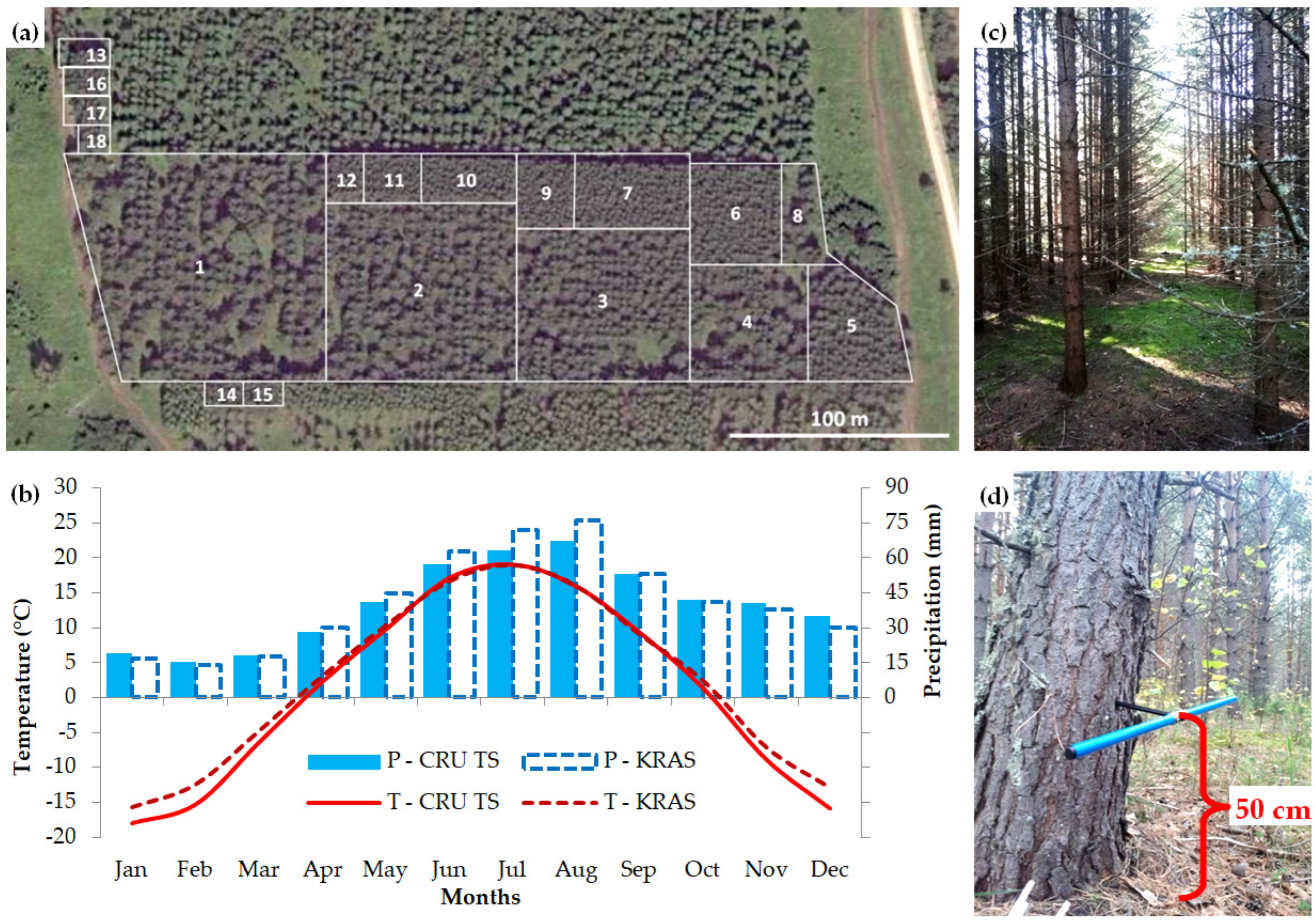
2.1. Study Area and Experimental Plantation
2.2. Data on Tree Morphometry and Radial Growth
2.3. Statistical Analysis
3. Results
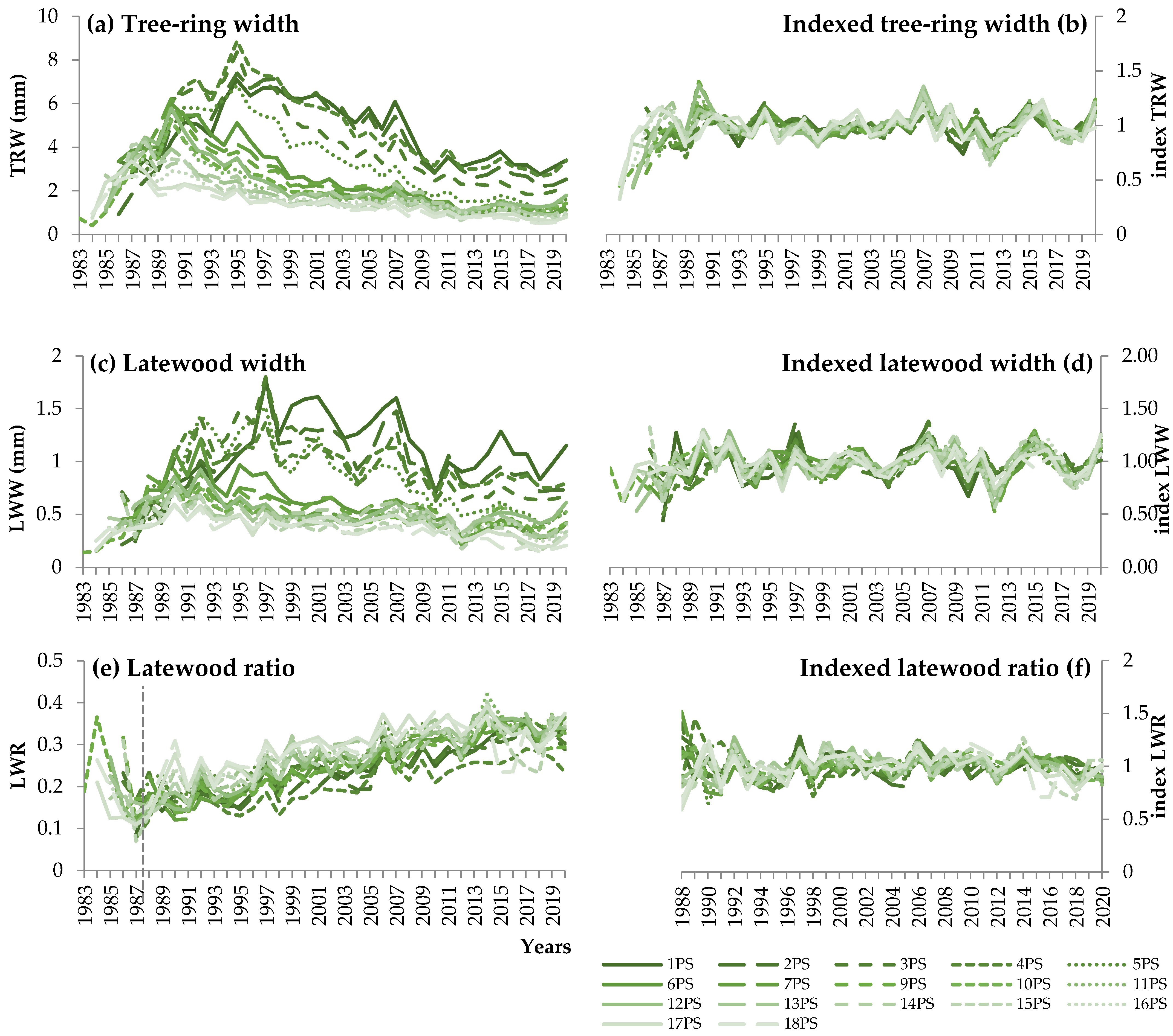
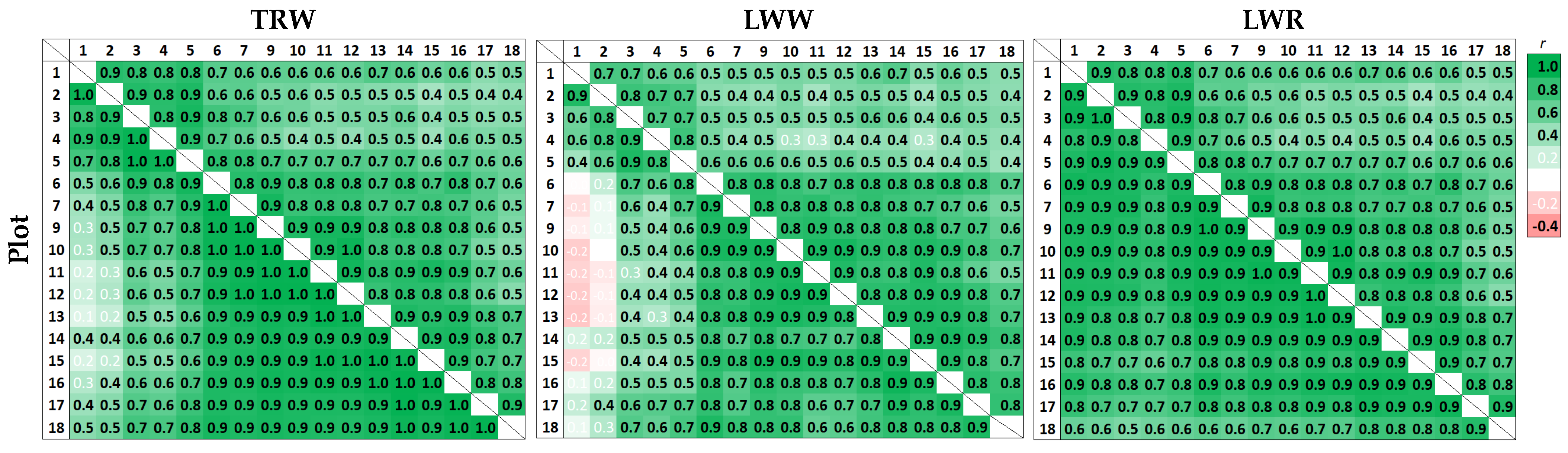
3.1. Dynamics of Pine Stand Density, Productivity, and Radial Growth Parameters
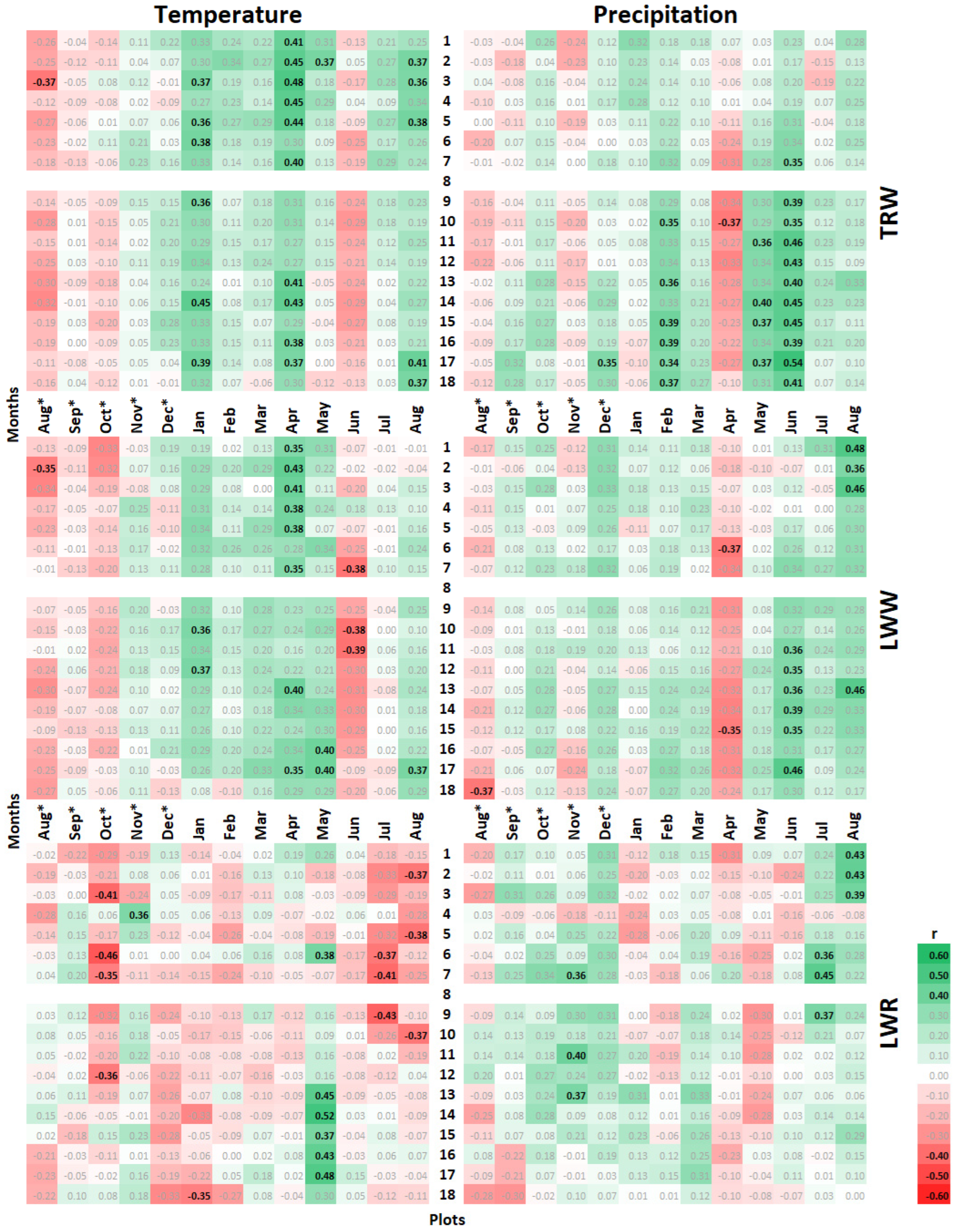
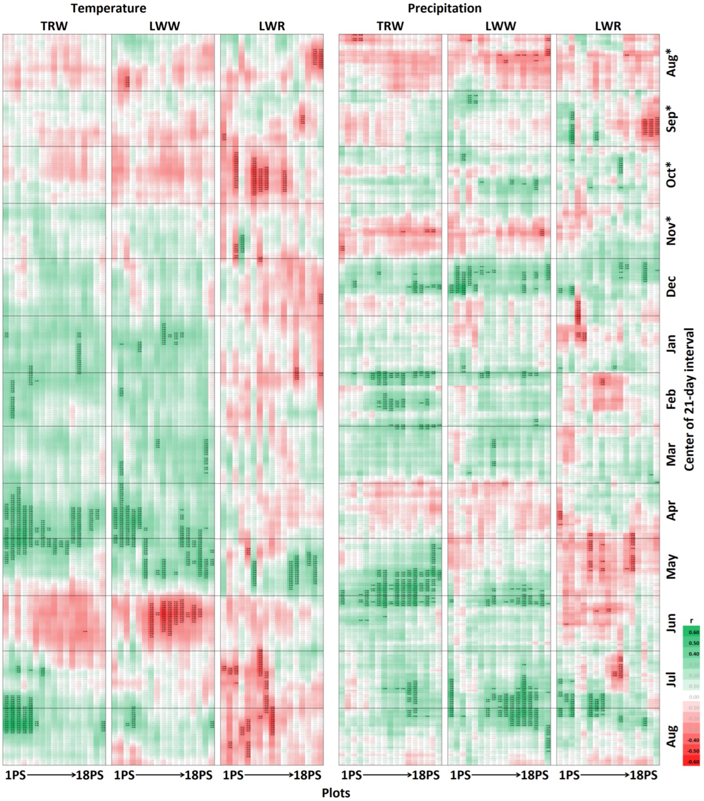
3.2. Climatic Response of Tree-Ring Parameters at Different Planting Densities
4. Discussion
4.1. Stand Density Dynamics and Tree and Stand Productivity
4.2. Climatic Response of Pine Radial Growth Parameters and its Dependence on the Stand Density
5. Conclusions
Author Contributions
Funding
Data Availability Statement
Conflicts of Interest
Appendix A

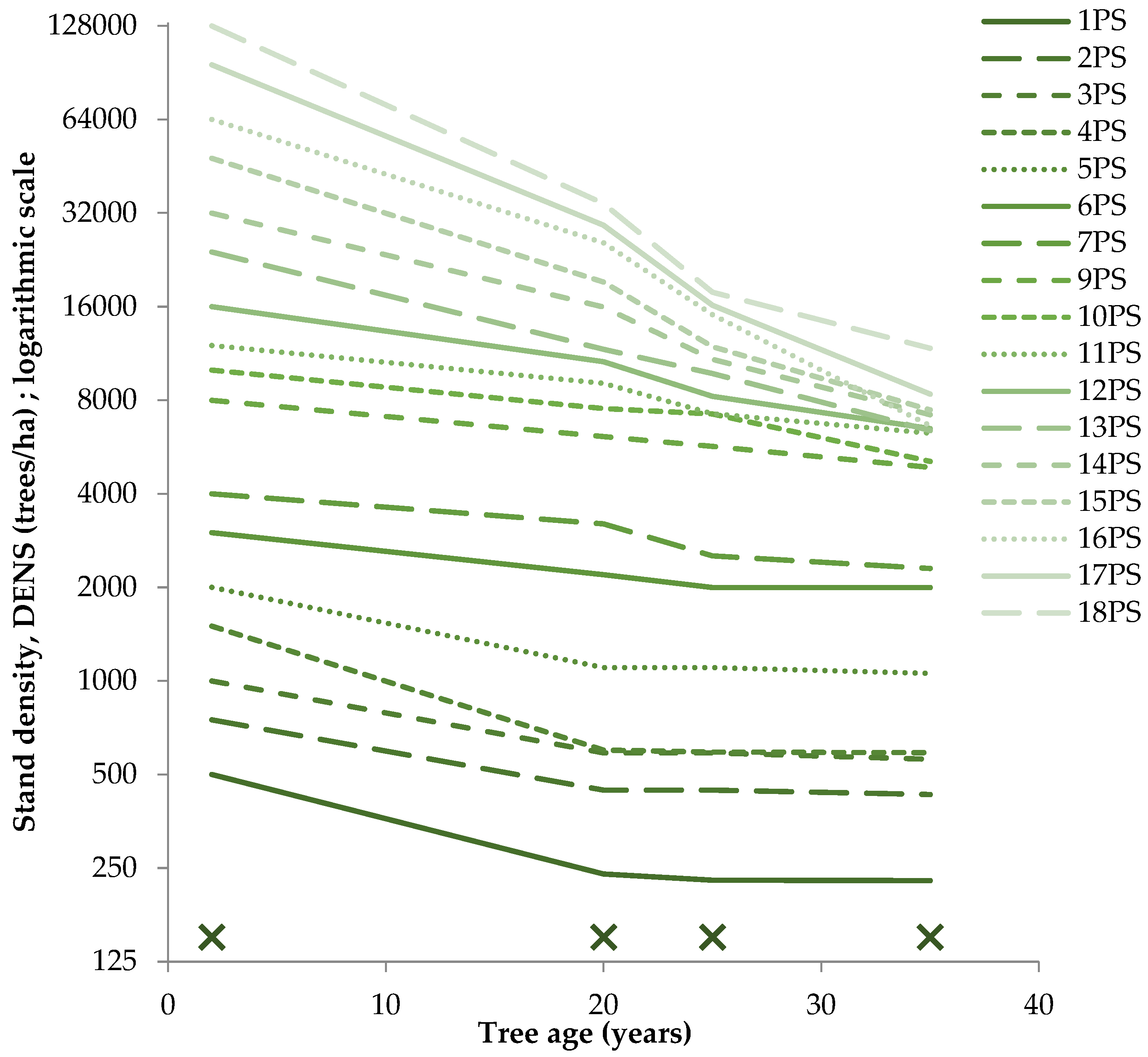
| Plot | Stand Density DENS (Trees/ha) at Ages A (Years) * | Function ** DENS = DENS0·exp[−a(A − A0)] | |||||
|---|---|---|---|---|---|---|---|
| A0 = 2 | 20 | 25 | 35 | a *** | R | R2 | |
| 1PS | 500 | 239 | 228 | 228 | −0.0274 | 0.911 | 0.830 |
| 2PS | 750 | 445 | 445 | 431 | −0.0190 | 0.915 | 0.837 |
| 3PS | 1000 | 567 | 567 | 560 | −0.0196 | 0.924 | 0.854 |
| 4PS | 1500 | 599 | 590 | 588 | −0.0330 | 0.899 | 0.808 |
| 5PS | 2000 | 1103 | 1103 | 1057 | −0.0218 | 0.919 | 0.844 |
| 6PS | 3000 | 2196 | 1997 | 1997 | −0.0136 | 0.947 | 0.897 |
| 7PS | 4000 | 3198 | 2523 | 2300 | −0.0157 | 0.968 | 0.938 |
| 9PS | 8000 | 6108 | 5683 | 4867 | −0.0139 | 0.999 | 0.999 |
| 10PS | 10,000 | 7524 | 7227 | 5085 | −0.0166 | 0.968 | 0.937 |
| 11PS | 12,000 | 9070 | 7236 | 6268 | −0.0182 | 0.983 | 0.966 |
| 12PS | 16,000 | 10,639 | 8236 | 6487 | −0.0250 | 0.991 | 0.983 |
| 13PS | 24,000 | 11,668 | 9742 | 6388 | −0.0370 | 0.999 | 0.999 |
| 14PS | 36,000 | 15,951 | 10,826 | 7181 | −0.0414 | 0.994 | 0.988 |
| 15PS | 48,000 | 19,207 | 11,890 | 7449 | −0.0525 | 0.995 | 0.990 |
| 16PS | 64,000 | 25,662 | 15,062 | 6627 | −0.0594 | 0.987 | 0.974 |
| 17PS | 96,000 | 29,243 | 16,115 | 8367 | −0.0682 | 0.996 | 0.992 |
| 18PS | 128,000 | 34,336 | 17,795 | 11,750 | −0.0706 | 0.990 | 0.980 |

References
- Edwards, D.P.; Tobias, J.A.; Sheil, D.; Meijaard, E.; Laurance, W.F. Maintaining ecosystem function and services in logged tropical forests. Trends Ecol. Evol. 2014, 29, 511–520. [Google Scholar] [CrossRef]
- Brockerhoff, E.G.; Barbaro, L.; Castagneyrol, B.; Forrester, D.I.; Gardiner, B.; Gonzalez-Olabarria, J.R.; Lyver, P.O.B.; Meurisse, N.; Oxbrough, A.; Taki, H.; et al. Forest biodiversity, ecosystem functioning and the provision of ecosystem services. Biodivers. Conserv. 2017, 26, 3005–3035. [Google Scholar] [CrossRef]
- Babst, F.; Carrer, M.; Poulter, B.; Urbinati, C.; Neuwirth, B.; Frank, D. 500 years of regional forest growth variability and links to climatic extreme events in Europe. Environ. Res. Lett. 2012, 7, 045705. [Google Scholar] [CrossRef]
- Pederson, N.; D’Amato, A.W.; Dyer, J.M.; Foster, D.R.; Goldblum, D.; Hart, J.L.; Hessl, A.E.; Iverson, L.R.; Jackson, S.T.; Martin-Benito, D.; et al. Climate remains an important driver of post-European vegetation change in the eastern United States. Glob. Chang. Biol. 2015, 21, 2105–2110. [Google Scholar] [CrossRef]
- Clark, J.S.; Iverson, L.; Woodall, C.W.; Allen, C.D.; Bell, D.M.; Bragg, D.C.; D’Amato, A.W.; Davis, F.W.; Hersh, M.H.; Ibanez, I.; et al. The impacts of increasing drought on forest dynamics, structure, and biodiversity in the United States. Glob. Chang. Biol. 2016, 22, 2329–2352. [Google Scholar] [CrossRef]
- Dyderski, M.K.; Paz, S.; Frelich, L.E.; Jagodzinski, A.M. How much does climate change threaten European forest tree species distributions? Glob. Change Biol. 2018, 24, 1150–1163. [Google Scholar] [CrossRef]
- Keenan, R.J.; Reams, G.A.; Achard, F.; de Freitas, J.V.; Grainger, A.; Lindquist, E. Dynamics of global forest area: Results from the FAO Global Forest Resources Assessment 2015. For. Ecol. Manag. 2015, 352, 9–20. [Google Scholar] [CrossRef]
- Rigling, A.; Waldner, P.O.; Forster, T.; Bräker, O.U.; Pouttu, A. Ecological interpretation of tree-ring width and intraannual density fluctuations in Pinus sylvestris on dry sites in the central Alps and Siberia. Can. J. For. Res. 2001, 31, 18–31. [Google Scholar] [CrossRef]
- Zhang, J.; Ritchie, M.W.; Maguire, D.A.; Oliver, W.W. Thinning ponderosa pine (Pinus ponderosa) stands reduces mortality while maintaining stand productivity. Can. J. For. Res. 2013, 43, 311–320. [Google Scholar] [CrossRef]
- Altman, J.; Fibich, P.; Santruckova, H.; Dolezal, J.; Stepanek, P.; Kopacek, J.; Hunova, I.; Oulehle, F.; Tumajer, J.; Cienciala, E. Environmental factors exert strong control over the climate-growth relationships of Picea abies in Central Europe. Sci. Total Environ. 2017, 609, 506–516. [Google Scholar] [CrossRef] [PubMed]
- Malanson, G.P. Mixed signals in trends of variance in high-elevation tree ring chronologies. J. Mt. Sci. 2017, 14, 1961–1968. [Google Scholar] [CrossRef]
- Morozov, G.; Guman, V. (Eds.) The Teaching of the Types of Plantings; Yurayt: Moscow, Russia, 2019; 371p. (In Russian) [Google Scholar]
- Huang, X.; Dai, D.; Xiang, Y.; Yan, Z.; Teng, M.; Wang, P.; Zhou, Z.; Zeng, L.; Xiao, W. Radial growth of Pinus massoniana is influenced by temperature, precipitation, and site conditions on the regional scale: A meta-analysis based on tree-ring width index. Ecol. Indic. 2021, 126, 107659. [Google Scholar] [CrossRef]
- Anderson-Teixeira, K.J.; Herrmann, V.; Rollinson, C.R.; Gonzalez, B.; Gonzalez-Akre, E.B.; Pederson, N.; Alexander, M.R.; Allen, C.D.; Alfaro-Sanchez, R.; Awada, T.; et al. Joint effects of climate, tree size, and year on annual tree growth derived from tree-ring records of ten globally distributed forests. Glob. Chang. Biol. 2022, 28, 245–266. [Google Scholar] [CrossRef]
- Vaganov, E.A.; Hughes, M.K.; Shashkin, A.V. Growth Dynamics of Conifer Tree Rings: Images of Past and Future Environments; Springer: Berlin/Heidelberg, Germany, 2006; 358p. [Google Scholar] [CrossRef]
- Chen, Y.; Cao, Y. Response of tree regeneration and understory plant species diversity to stand density in mature Pinus tabulaeformis plantations in the hilly area of the Loess Plateau, China. Ecol. Eng. 2014, 73, 238–245. [Google Scholar] [CrossRef]
- Jiao, L.; Jiang, Y.; Wang, M.; Zhang, W.; Zhang, Y. Age-effect radial growth responses of Picea schrenkiana to climate change in the eastern Tianshan Mountains, Northwest China. Forests 2017, 8, 294. [Google Scholar] [CrossRef]
- Perry, D.A. The competition process in forest stands. In Attributes of Trees as Crop Plants; Cannell, M.G.R., Jackson, J.E., Eds.; Institute of Terrestial Ecology: Abbots Ripton, UK, 1985; pp. 481–506. [Google Scholar]
- Sheriff, D.W. Responses of carbon gain and growth of Pinus radiata stands to thinning and fertilizing. Tree Physiol. 1996, 16, 527–536. [Google Scholar] [CrossRef] [PubMed]
- Pshenichnikova, L.S. Pine growth in the experimental planting of different density. Lesn. Z. For. J. 2001, 1, 25–31, (In Russian with English abstract). [Google Scholar]
- Kazmierczak, K. Selected measures of the growth space of a single tree in maturing pine stand. Sylwan 2009, 153, 298–303, (In Polish with English abstract). [Google Scholar]
- Lundqvist, L.; Elfving, B. Influence of biomechanics and growing space on tree growth in young Pinus sylvestris stands. For. Ecol. Manag. 2010, 260, 2143–2147. [Google Scholar] [CrossRef]
- Gómez-Aparicio, L.; García-Valdes, R.; Ruiz-Benito, P.; Zavala, M.A. Disentangling the relative importance of climate, size and competition on tree growth in Iberian forests: Implications for management under global change. Glob. Change Biol. 2011, 17, 2400–2414. [Google Scholar] [CrossRef]
- Kuzmichev, V.V.; Pshenichnikova, L.S. Growth of Scots pine stands planted in a range of density in southern taiga of Krasnoyarsk region. Hvojnye Borealnoj Zony 2014, 32, 83–88, (In Russian with English abstract). [Google Scholar]
- Burkhart, H.E. Comparison of maximum size–density relationships based on alternate stand attributes for predicting tree numbers and stand growth. For. Ecol. Manag. 2013, 289, 404–408. [Google Scholar] [CrossRef]
- Martín-Benito, D.; del Río, M.; Heinrich, I.; Helle, G.; Cañellas, I. Response of climate-growth relationships and water use efficiency to thinning in a Pinus nigra afforestation. For. Ecol. Manag. 2010, 259, 967–975. [Google Scholar] [CrossRef]
- Wertz, B.; Bembenek, M.; Karaszewski, Z.; Ochal, W.; Skorupski, M.; Strzelinski, P.; Wegiel, A.; Mederski, P.S. Impact of stand density and tree social status on aboveground biomass allocation of Scots pine Pinus sylvestris L. Forests 2020, 11, 765. [Google Scholar] [CrossRef]
- Cochran, P.H. Examples of Mortality and Reduced Annual Increments of White Fir Induced by Drought, Insects, and Disease at Different Stand Densities; USDA Forest Service, Pacific Northwest Experiment Station: Portland, OR, USA, 1998; 19p. [CrossRef]
- Latham, P.; Tappeiner, J. Response of old-growth conifers to reduction in stand density in western Oregon forests. Tree Physiol. 2002, 22, 137–146. [Google Scholar] [CrossRef] [PubMed]
- D’Amato, A.W.; Bradford, J.B.; Fraver, S.; Palik, B.J. Effects of thinning on drought vulnerability and climate response in north temperate forest ecosystems. Ecol. Appl. 2013, 23, 1735–1742. [Google Scholar] [CrossRef]
- Bello, J.; Vallet, P.; Perot, T.; Balandier, P.; Seigner, V.; Perret, S.; Couteau, C.; Korboulewsky, N. How do mixing tree species and stand density affect seasonal radial growth during drought events? For. Ecol. Manag. 2019, 432, 436–445. [Google Scholar] [CrossRef]
- Piutti, E.; Cescatti, A. A quantitative analysis of the interactions between climatic response and intraspecific competition in European beech. Can. J. For. Res. 1997, 27, 277–284. [Google Scholar] [CrossRef]
- Zeide, B. How to measure stand density. Trees 2005, 19, 1–14. [Google Scholar] [CrossRef]
- Buzykin, A.I.; Pshenichnikova, L.S. Influence of Scots pine stands of different planting densities on radial growth. Hvojnye Borealnoj Zony 2011, 28, 188–192, (In Russian with English abstract). [Google Scholar]
- Trouve, R.; Bontemps, J.D.; Seynave, I.; Collet, C.; Lebourgeois, F. Stand density, tree social status and water stress influence allocation in height and diameter growth of Quercus petraea (Liebl.). Tree Physiol. 2015, 35, 1035–1046. [Google Scholar] [CrossRef] [PubMed]
- Steckel, M.; Moser, W.K.; del Río, M.; Pretzsch, H. Implications of reduced stand density on tree growth and drought susceptibility: A study of three species under varying climate. Forests 2020, 11, 627. [Google Scholar] [CrossRef]
- Weiner, J. Size hierarchies in experimental populations of annual plants. Ecology 1985, 66, 743–752. [Google Scholar] [CrossRef]
- Silvertown, J.; Charlesworth, D. Introduction to Plant Population Biology, 4th ed.; Wiley-Blackwell: Hoboken, NJ, USA, 2009; 368p. [Google Scholar]
- Chhetri, P.K.; Bista, R.; Shrestha, K.B. How does the stand structure of treeline-forming species shape the treeline ecotone in different regions of the Nepal Himalayas? J. Mt. Sci. 2020, 17, 2354–2368. [Google Scholar] [CrossRef]
- Chapin, F.S.; Matson, P.A.; Mooney, H.A. Principles of Terrestrial Ecosystem Ecology; Springer: Berlin/Heidelberg, Germany, 2011; 529p. [Google Scholar] [CrossRef]
- Kerhoulas, L.P.; Kolb, T.E.; Koch, G.W. Tree size, stand density, and the source of water used across seasons by ponderosa pine in northern Arizona. For. Ecol. Manag. 2013, 289, 425–433. [Google Scholar] [CrossRef]
- Nilsson, U.; Albrektson, A. Productivity of needles and allocation of growth in young Scots pine trees of different competitive status. For. Ecol. Manag. 1993, 62, 173–187. [Google Scholar] [CrossRef]
- Mäkinen, H. Effect of intertree competition on biomass production of Pinus sylvestris (L.) half-sib families. For. Ecol. Manag. 1996, 86, 105–112. [Google Scholar] [CrossRef]
- Ochal, W.; Grabczynski, S.; Orzel, S.; Wertz, B.; Socha, J. Aboveground biomass allocation in Scots pines of different biosocial positions in the stand. Sylwan 2013, 157, 737–746, (In Polish with English abstract). [Google Scholar]
- Zobel, B.J.; Van Buijtenen, J.P. Wood Variation: Its Causes and Control; Springer: Berlin/Heidelberg, Germany, 1989; 363p. [Google Scholar]
- Martin-Benito, D.; Cherubini, P.; del Rio, M.; Canellas, I. Growth response to climate and drought in Pinus nigra Arn. trees of different crown classes. Trees 2008, 22, 363–373. [Google Scholar] [CrossRef]
- Martinez-Vilalta, J.; Lopez, B.C.; Loepfe, L.; Lloret, F. Stand- and tree-level determinants of the drought response of Scots pine radial growth. Oecologia 2012, 168, 877–888. [Google Scholar] [CrossRef] [PubMed]
- Plauborg, K.U. Analysis of radial growth responses to changes in stand density for four tree species. For. Ecol. Manag. 2004, 188, 65–75. [Google Scholar] [CrossRef]
- Leibundgut, H. Unsere Waldbäume. Eigenschaften und Leben [Our Forest Trees. Properties and Life]; Verlag Huber: Frauenfeld, Switzerland, 1984; 168p. (In German) [Google Scholar]
- Schweingruber, F.H. Trees and Wood in Dendrochronology; Springer: Berlin/Heidelberg, Germany, 1993; 402p. [Google Scholar] [CrossRef]
- Locosselli, G.M.; Buckeridge, M.S.; Moreira, M.Z.; Ceccantini, G. A multi-proxy dendroecological analysis of two tropical species (Hymenaea spp., Leguminosae) growing in a vegetation mosaic. Trees 2013, 27, 25–36. [Google Scholar] [CrossRef]
- Puettmann, K.J. Silvicultural challenges and options in the context of global change: “Simple” fixes and opportunities for new management approaches. J. For. 2011, 109, 321–331. [Google Scholar] [CrossRef]
- Buzykin, A.I.; Pshenichnikova, L.S.; Sobachkin, D.S.; Sobachkin, R.S. Natural thinning of young trees in experimental pine plantings of different density. Hvojnye Borealnoj Zony 2008, 25, 244–249, (In Russian with English abstract). [Google Scholar]
- Pshenichnikova, L.S. Productivity of young pine forests of different density. In Factors of Forest Productivity: Collected Works; Nauka: Novosibirsk, Russia, 1978; pp. 36–52. (In Russian) [Google Scholar]
- Pobedinsky, A.V. Study of Reforestation Processes; Nauka: Moscow, USSR, 1966; 60p. (In Russian) [Google Scholar]
- Moiseev, V.S. Inventory of Saplings; Forest Engineering Academy: Leningrad, USSR, 1971; 344p. (In Russian) [Google Scholar]
- Buzykin, A.I. On the productivity of forests and the levels of its regulation. In Problems of Forest Science in Siberia; Nauka: Moscow, USSR, 1977; pp. 7–24. (In Russian) [Google Scholar]
- Buzykin, A.I.; Pshenichnikova, L.S. Influence of density on the morphostructure and productivity of pine plantations. Lesovedenie [For. Sci.] 1999, 3, 38–43. (In Russian) [Google Scholar]
- Peng, P.H.; Kuo, C.H.; Wei, C.H.; Hsieh, Y.T.; Chen, J.C. The relationship between breast height form factor and form quotient of Liquidambar formosana in the Eastern part of Taiwan. Forests 2022, 13, 1111. [Google Scholar] [CrossRef]
- Tishin, D.V. Assessment of Tree Stand Productivity; Educational-Methodical Manual; Kazan University: Kazan, Russia, 2011; 31p. (In Russian) [Google Scholar]
- Coomes, D.A.; Allen, R.B. Mortality and tree-size distributions in natural mixed-age forests. J. Ecol. 2007, 95, 27–40. [Google Scholar] [CrossRef]
- Chen, H.Y.H.; Fu, S.; Monserud, R.A.; Gillies, I. Relative size and stand age determine Pinus banksiana mortality. For. Ecol. Manag. 2008, 255, 3980–3984. [Google Scholar] [CrossRef]
- Cook, E.R.; Kairiukstis, L.A. (Eds.) Methods of Dendrochronology. Application in Environmental Sciences; Kluwer Academic Publishers: Dordrecht, Germany, 1990; 394p. [Google Scholar] [CrossRef]
- Rinn, F. TSAP-Win: Time Series Analysis and Presentation for Dendrochronology and Related Applications: User Reference; RINNTECH: Heidelberg, Germany, 2003; 91p. [Google Scholar]
- Holmes, R.L. Computer-assisted quality control in tree-ring dating and measurement. Tree-Ring Bull. 1983, 43, 69–78. [Google Scholar]
- Cook, E.R.; Krusic, P.J. Program ARSTAN: A Tree-Ring Standardization Program Based on Detrending and Autoregressive Time Series Modeling, with Interactive Graphics; Lamont-Doherty Earth Observatory, Columbia University: Palisades, NY, USA, 2005; 14p. [Google Scholar]
- Meko, D.M.; Baisan, C.H. Pilot study of latewood-width of conifers as an indicator of variability of summer rainfall in the North American monsoon region. Int. J. Climatol. 2001, 21, 697–708. [Google Scholar] [CrossRef]
- Wigley, T.M.L.; Briffa, K.R.; Jones, P.D. On the average value of correlated time series, with applications in dendroclimatology and hydrometeorology. J. Clim. Appl. Met. 1984, 23, 201–213. [Google Scholar] [CrossRef]
- Ford, E.D. Branching, crown structure and the control of timber production. In Attributes of Trees as Crop Plants; Cannell, M.G.R., Jackson, J.E., Eds.; Institute of Terrestrial Ecology: Abbotts Ripton, UK, 1985; pp. 228–252. [Google Scholar]
- Oliver, C.D.; Larson, B.C. Forest Stand Dynamics; McGraw-Hill, Inc.: New York, NY, USA, 1996; 467p. [Google Scholar]
- Xue, L.; Chen, F.X.; Feng, H.F. Time-trajectory of mean component weight and density in self-thinning Pinus densiflora stands. Eur. J. For. Res. 2010, 129, 1027–1035. [Google Scholar] [CrossRef]
- Sola, G.; Marchelli, P.; Gallo, L.; Chauchard, L.; El Mujtar, V. Stand development stages and recruitment patterns influence fine-scale spatial genetic structure in two Patagonian Nothofagus species. Ann. For. Sci. 2022, 79, 21. [Google Scholar] [CrossRef]
- Lane, B.; Prusinkiewicz, P. Generating spatial distributions for multilevel models of plant communities. In Proceedings of the Graphics Interface 2002, Calgary, AL, Canada, 27–29 May 2002; pp. 69–80. [Google Scholar]
- Morris, E. How does fertility of the substrate affect intraspecific competition? Evidence and synthesis from self-thinning. Ecol. Res. 2003, 18, 287–305. [Google Scholar] [CrossRef]
- Kamara, M.; Kamruzzaman, M. Self-thinning process, dynamics of aboveground biomass, and stand structure in overcrowded mangrove Kandelia obovata stand. Reg. Studies Mar. Sci. 2020, 38, 101375. [Google Scholar] [CrossRef]
- Waring, R.H. Characteristics of trees predisposed to die: Stress causes distinctive changes in photosynthate allocation. BioScience 1987, 37, 569–574. [Google Scholar] [CrossRef]
- Baldwin, V.C., Jr.; Peterson, K.D.; Clark, A., III; Ferguson, R.B.; Strub, M.R.; Bower, D.R. The effects of spacing and thinning on stand and tree characteristics of 38-year-old loblolly pine. For. Ecol. Manag. 2000, 137, 91–102. [Google Scholar] [CrossRef]
- Zhang, S.Y.; Lei, Y.C.; Bowling, C. Quantifying stem quality characteristics in relation to initial spacing and modeling their relationship with tree characteristics in black spruce (Picea mariana). North. J. Appl. For. 2005, 22, 85–93. [Google Scholar] [CrossRef]
- del Río, M.; Bravo-Oviedo, A.; Ruiz-Peinado, R.; Condes, S. Tree allometry variation in response to intra-and inter-specific competitions. Trees 2019, 33, 121–138. [Google Scholar] [CrossRef]
- Woodruff, D.R.; Bond, B.J.; Ritchie, G.A.; Scott, W. Effects of stand density on the growth of young Douglas-fir trees. Can. J. For. Res. 2002, 32, 420–427. [Google Scholar] [CrossRef]
- Tepley, A.J.; Swanson, F.J.; Spies, T.A. Post-fire tree establishment and early cohort development in conifer forests of the western Cascades of Oregon, USA. Ecosphere 2014, 5, 1–23. [Google Scholar] [CrossRef]
- Abbas, A.M.; Al-Kahtani, M.; Novak, S.J.; Soliman, W.S. Abundance, distribution, and growth characteristics of three keystone Vachellia trees in Gebel Elba National Park, south-eastern Egypt. Sci. Rep. 2021, 11, 1284. [Google Scholar] [CrossRef]
- Reineke, L.H. Perfecting a stand-density index for even-aged forests. J. Agric. Res. 1933, 46, 627–638. [Google Scholar]
- Yoda, K.; Kira, T.; Ogawa, H.; Hozumi, K. Self-thinning in overcrowded pure stands under cultivated and natural conditions (Intraspecific competition among higher plants XI). J. Inst. Polytech. Osaka City Univ. Ser. D 1963, 14, 107–129. [Google Scholar]
- Lonsdale, W.M. The self-thinning rule: Dead or alive? Ecology 1990, 71, 1373–1388. [Google Scholar] [CrossRef]
- Pretzsch, H.; Biber, P. A re-evaluation of Reineke’s rule and stand density index. For. Sci. 2005, 51, 304–320. [Google Scholar] [CrossRef]
- Zhang, W.P.; Zhao, L.; Larjavaara, M.; Morris, E.C.; Sterck, F.J.; Wang, G.X. Height-diameter allometric relationships for seedlings and trees across China. Acta Oecol. 2020, 108, 103621. [Google Scholar] [CrossRef]
- Zhang, W.P.; Jia, X.; Morris, E.C.; Bai, Y.Y.; Wang, G.X. Stem, branch and leaf biomass-density relationships in forest communities. Ecol. Res. 2012, 27, 819–825. [Google Scholar] [CrossRef]
- Zhang, J.; Oliver, W.W.; Ritchie, M.W. Effect of stand densities on stand dynamics in white fir (Abies concolor) forests in northeast California, USA. For. Ecol. Manag. 2007, 244, 50–59. [Google Scholar] [CrossRef]
- Isaac-Renton, M.; Stoehr, M.; Statland, C.B.; Woods, J. Tree breeding and silviculture: Douglas-fir volume gains with minimal wood quality loss under variable planting densities. For. Ecol. Manag. 2020, 465, 118094. [Google Scholar] [CrossRef]
- Skovsgaard, J.A.; Vanclay, J.K. Forest site productivity: A review of the evolution of dendrometric concepts for even-aged stands. For. Int. J. For. Res. 2008, 81, 13–31. [Google Scholar] [CrossRef]
- Burkhart, H.E.; Tome, M. Modeling Forest Trees and Stands; Springer: Dordrecht, Germany, 2012; 458p. [Google Scholar] [CrossRef]
- Kholdaenko, Y.A.; Belokopytova, L.V.; Zhirnova, D.F.; Upadhyay, K.K.; Tripathi, S.K.; Koshurnikova, N.N.; Sobachkin, R.S.; Babushkina, E.A.; Vaganov, E.A. Stand density effects on tree growth and climatic response in Picea obovata Ledeb. plantations. For. Ecol. Manag. 2022, 519, 120349. [Google Scholar] [CrossRef]
- Mäkinen, H.; Isomäki, A. Thinning intensity and long-term changes in increment and stem form of Norway spruce trees. For. Ecol. Manag. 2004, 201, 295–309. [Google Scholar] [CrossRef]
- Weiskittel, A.R.; Maguire, D.A.; Monserud, R.A. Modeling crown structural responses to competing vegetation control, thinning, fertilization, and Swiss needle cast in coastal Douglas-fir of the Pacific Northwest, USA. For. Ecol. Manag. 2007, 245, 96–109. [Google Scholar] [CrossRef]
- Kofman, G.B. Growth and Form of Trees; Nauka: Novosibirsk, Russia, 1986; 211p. (In Russian) [Google Scholar]
- Gartner, B.L. Patterns of xylem variation within a tree and their hydraulic and mechanical consequences. In Plant Stems: Physiology and Functional Morphology; Academic Press: Cambridge, MA, USA, 1995; pp. 125–149. [Google Scholar] [CrossRef]
- Sarkhad, M.; Ishiguri, F.; Nezu, I.; Aiso, H.; Ngadianto, A.; Tumenjargal, B.; Baasan, B.; Chultem, G.; Ohshima, J.; Yokota, S. Preliminary evaluation of anatomical characteristics of four common Mongolian softwoods. For. Sci. Technol. 2022, 18, 87–97. [Google Scholar] [CrossRef]
- Domec, J.C.; Gartner, B.L. Age-and position-related changes in hydraulic versus mechanical dysfunction of xylem: Inferring the design criteria for Douglas-fir wood structure. Tree Physiol. 2002, 22, 91–104. [Google Scholar] [CrossRef] [PubMed]
- Liu, Y.; Shi, J.; Shishov, V.; Vaganov, E.; Yang, Y.; Cai, Q.; Sun, J.; Wang, L.; Djanseitov, I. Reconstruction of May–July precipitation in the north Helan Mountain, Inner Mongolia since AD 1726 from tree-ring late-wood widths. Chin. Sci. Bull. 2004, 49, 405–409. [Google Scholar] [CrossRef]
- Lebourgeois, F. Climatic signals in earlywood, latewood and total ring width of Corsican pine from western France. Ann. For. Sci. 2000, 57, 155–164. [Google Scholar] [CrossRef]
- Zhang, S.Y. Variations and correlations of various ring width and ring density features in European oak: Implications in dendroclimatology. Wood Sci. Technol. 1997, 31, 63–72. [Google Scholar] [CrossRef]
- Savva, Y.V.; Schweingruber, F.H.; Vaganov, E.A.; Milyutin, L.I. Influence of climate changes on tree-ring characteristics of Scots pine provenances in southern Siberia (forest-steppe). IAWA J. 2003, 24, 371–383. [Google Scholar] [CrossRef]
- Bauwe, A.; Koch, M.; Kallweit, R.; Konopatzky, A.; Strohbach, B.; Lennartz, B. Tree-ring growth response of Scots pine (Pinus sylvestris L.) to climate and soil water availability in the lowlands of North-Eastern Germany. Balt. For. 2013, 19, 212–225. [Google Scholar]
- Voltas, J.; Aguilera, M.; Gutierrez, E.; Shestakova, T.A. Shared drought responses among conifer species in the middle Siberian taiga are uncoupled from their contrasting water-use efficiency trajectories. Sci. Total Environ. 2020, 720, 137590. [Google Scholar] [CrossRef] [PubMed]
- Arzac, A.; Tabakova, M.A.; Khotcinskaia, K.; Koteneva, A.; Kirdyanov, A.V.; Olano, J.M. Linking tree growth and intra-annual density fluctuations to climate in suppressed and dominant Pinus sylvestris L. trees in the forest-steppe of Southern Siberia. Dendrochronologia 2021, 67, 125842. [Google Scholar] [CrossRef]
- Kolar, T.; Kusbach, A.; Cermak, P.; Sterba, T.; Batkhuu, E.; Rybnicek, M. Climate and wildfire effects on radial growth of Pinus sylvestris in the Khan Khentii Mountains, north-central Mongolia. J. Arid Environ. 2020, 182, 104223. [Google Scholar] [CrossRef]
- Zhirnova, D.F.; Belokopytova, L.V.; Meko, D.M.; Babushkina, E.A.; Vaganov, E.A. Climate change and tree growth in the Khakass-Minusinsk Depression (South Siberia) impacted by large water reservoirs. Sci. Rep. 2021, 11, 14266. [Google Scholar] [CrossRef]
- Kargas, G.; Kerkides, P.; Poulovassilis, A. Infiltration of rain water in semi-arid areas under three land surface treatments. Soil Tillage Res. 2012, 120, 15–24. [Google Scholar] [CrossRef]
- Fritts, H.C. Growth-rings of trees: Their correlation with climate: Patterns of ring widths in trees in semiarid sites depend on climate-controlled physiological factors. Science 1966, 154, 973–979. [Google Scholar] [CrossRef]
- Allen, C.D.; Macalady, A.K.; Chenchouni, H.; Bachelet, D.; McDowell, N.; Vennetier, M.; Kitzberger, T.; Rigling, A.; Breshears, D.D.; Hogg, E.H.; et al. A global overview of drought and heat-induced tree mortality reveals emerging climate change risks for forests. For. Ecol. Manag. 2010, 259, 660–684. [Google Scholar] [CrossRef]
- Liu, H.; Park Williams, A.; Allen, C.D.; Guo, D.; Wu, X.; Anenkhonov, O.A.; Liang, E.; Sandanov, D.V.; Yin, Y.; Qi, Z.; et al. Rapid warming accelerates tree growth decline in semi-arid forests of Inner Asia. Glob. Change Biol. 2013, 19, 2500–2510. [Google Scholar] [CrossRef] [PubMed]
- Long, A.L. Drought. In Disturbance and Sustainability in Forests of the Western United States; Barrett, T.M., Robertson, G.C., Eds.; USDA Forest Service, Pacific Northwest Research Station: Portland, OR, USA, 2021; pp. 67–79. [Google Scholar]
- Yasmeen, S.; Wang, X.; Zhao, H.; Zhu, L.; Yuan, D.; Li, Z.; Zhang, Y.; Ahmad, S.; Han, S. Contrasting climate-growth relationship between Larix gmelinii and Pinus sylvestris var. mongolica along a latitudinal gradient in Daxing’an Mountains, China. Dendrochronologia 2019, 58, 125645. [Google Scholar] [CrossRef]
- Agafonov, L.I.; Gurskaya, M.A.; Kukarskih, V.V.; Bubnov, M.O.; Devi, N.M.; Galimova, A.A. Insular pine forests of the Southern Urals and ribbon pine forests of the Altai as objects of dendroclimatic research. Russ. J. Ecol. 2021, 52, 349–357. [Google Scholar] [CrossRef]
- Arzac, A.; Tychkov, I.; Rubtsov, A.; Tabakova, M.A.; Brezhnev, R.; Koshurnikova, N.; Knorre, A.; Büntgen, U. Phenological shifts compensate warming-induced drought stress in southern Siberian Scots pines. Eur. J. For. Res. 2021, 140, 1487–1498. [Google Scholar] [CrossRef]
- Jayawickrama, K.J.; McKeand, S.E.; Jett, J.B.; Wheeler, E.A. Date of earlywood-latewood transition in provenances and families of loblolly pine, and its relationship to growth phenology and juvenile wood specific gravity. Can. J. For. Res. 1997, 27, 1245–1253. [Google Scholar] [CrossRef]
- Yang, B.; He, M.; Shishov, V.; Tychkov, I.; Vaganov, E.; Rossi, S.; Ljungqvist, F.C.; Bräuning, A.; Grießinger, J. New perspective on spring vegetation phenology and global climate change based on Tibetan Plateau tree-ring data. PNAS 2017, 114, 6966–6971. [Google Scholar] [CrossRef] [PubMed]
- Fonti, M.V.; Babushkina, E.A.; Zhirnova, D.F.; Vaganov, E.A. Xylogenesis of Scots pine in an uneven-aged stand of the Minusinsk Depression (Southern Siberia). J. Sib. Fed. Univ. Biol. 2020, 13, 197–207. [Google Scholar] [CrossRef]
- Gricar, J.; Cufar, K.; Eler, K.; Gryc, V.; Vavrcík, H.; De Luis, M.; Prislan, P. Transition dates from earlywood to latewood and early phloem to late phloem in Norway spruce. Forests 2021, 12, 331. [Google Scholar] [CrossRef]
- Babushkina, E.A.; Sitnikov, G.A.; Upadhyay, K.K.; Zhirnova, D.F.; Zelenov, G.K.; Vaganov, E.A.; Belokopytova, L.V. Seasonal growth of pine tree rings: Comparison of direct observations and simulation. Forests 2022, 13, 1978. [Google Scholar] [CrossRef]
- Deleuze, C.; Herve, J.C.; Colin, F.; Ribeyrolles, L. Modelling crown shape of Picea abies: Spacing effects. Can. J. For. Res. 1996, 26, 1957–1966. [Google Scholar] [CrossRef]
- Misson, L.; Nicault, A.; Guiot, J. Effects of different thinning intensities on drought response in Norway spruce (Picea abies (L.) Karst.). For. Ecol. Manag. 2003, 183, 47–60. [Google Scholar] [CrossRef]
- Sohn, J.A.; Gebhardt, T.; Ammer, C.; Bauhus, J.; Haberle, K.H.; Matyssek, R.; Grams, T.E.E. Mitigation of drought by thinning: Short-term and long-term effects on growth and physiological performance of Norway spruce (Picea abies). For. Ecol. Manag. 2013, 308, 188–197. [Google Scholar] [CrossRef]
- Olivar, J.; Bogino, S.; Rathgeber, C.; Bonnesoeur, V.; Bravo, F. Thinning has a positive effect on growth dynamics and growth–climate relationships in Aleppo pine (Pinus halepensis) trees of different crown classes. Ann. For. Sci. 2014, 71, 395–404. [Google Scholar] [CrossRef]
- Peltola, H.; Kilpeläinen, A.; Sauvala, K.; Räisänen, T.; Ikonen, V.P. Effects of early thinning regime and tree status on the radial growth and wood density of Scots pine. Silva Fenn. 2007, 41, 489–505. [Google Scholar] [CrossRef]
- Perevalova, E.A. Drought effect on the cambial activity of Scots pine in stands of different planting density. In Forestry Universities in the Implementation of the Concept of the Engineering Education Revival: Socio-Economic and Environmental Problems of the Forestry Complex; Ural State Forest Engineering University: Ekaterinburg, Russia, 2019; pp. 219–221, (In Russian with English abstract). [Google Scholar]
- Coomes, D.A.; Allen, R.B. Effects of size, competition and altitude on tree growth. J. Ecol. 2007, 95, 1084–1097. [Google Scholar] [CrossRef]
- Aussenac, G. Interactions between forest stands and microclimate: Ecophysiological aspects and consequences for silviculture. Ann. For. Sci. 2000, 57, 287–301. [Google Scholar] [CrossRef]
- Liu, J.; Chen, J.M.; Cihlar, J. Mapping evapotranspiration based on remote sensing: An application to Canada’s landmass. Water Resour. Res. 2003, 39, 1189. [Google Scholar] [CrossRef]
- Moreno-Gutierrez, C.; Battipaglia, G.; Cherubini, P.; Saurer, M.; Nicolas, E.; Contreras, S.; Querejeta, J.I. Stand structure modulates the long-term vulnerability of Pinus halepensis to climatic drought in a semiarid Mediterranean ecosystem. Plant Cell Environ. 2012, 35, 1026–1039. [Google Scholar] [CrossRef] [PubMed]
- Van Den Brakel, J.A.; Visser, H. The influence of environmental conditions on tree-ring series of Norway spruce for different canopy and vitality classes. For. Sci. 1996, 42, 206–219. [Google Scholar] [CrossRef]
- Merian, P.; Lebourgeois, F. Size-mediated climate–growth relationships in temperate forests: A multi-species analysis. For. Ecol. Manag. 2011, 261, 1382–1391. [Google Scholar] [CrossRef]
- Campelo, F.; Vieira, J.; Nabais, C. Tree-ring growth and intra-annual density fluctuations of Pinus pinaster responses to climate: Does size matter? Trees 2013, 27, 763–772. [Google Scholar] [CrossRef]
- Ford, K.R.; Breckheimer, I.K.; Franklin, J.F.; Freund, J.A.; Kroiss, S.J.; Larson, A.J.; Theobald, E.J.; HilleRisLambers, J. Competition alters tree growth responses to climate at individual and stand scales. Can. J. For. Res. 2017, 47, 53–62. [Google Scholar] [CrossRef]
- Campbell, E.M.; Magnussen, S.; Antos, J.A.; Parish, R. Size-, species-, and site-specific tree growth responses to climate variability in old-growth subalpine forests. Ecosphere 2021, 12, e03529. [Google Scholar] [CrossRef]
- Babushkina, E.A.; Vaganov, E.A.; Belokopytova, L.V.; Shishov, V.V.; Grachev, A.M. Competitive strength effect in the climate response of Scots pine radial growth in south-central Siberia forest-steppe. Tree-Ring Res. 2015, 71, 106–117. [Google Scholar] [CrossRef]
- Matyshak, G.V.; Goncharova, O.Y.; Bogatyrev, L.G.; Riazantseva, M.I. Influence of plant cover on hydrothermal conditions in soils of large lysimeters of the MSU soil station: Results of a 60-year experiment. Mosc. Univ. Soil Sci. Bull. 2021, 76, 134–139. [Google Scholar] [CrossRef]
- Duyar, A. The effects of forest canopy cover and altitude on snow accumulation and melting in the upper watersheds. Fresenius Environ. Bull. 2018, 27, 9642–9649. [Google Scholar]
- Chen, L.; Chen, Z.; Jia, G.; Zhou, J.; Zhao, J.; Zhang, Z. Influences of forest cover on soil freeze-thaw dynamics and greenhouse gas emissions through the regulation of snow regimes: A comparison study of the farmland and forest plantation. Sci. Total Environ. 2020, 726, 138403. [Google Scholar] [CrossRef] [PubMed]
- Fu, Q.; Hou, R.; Li, T.; Yan, P.; Ma, Z. The critical depth of freeze-thaw soil under different types of snow cover. Water 2017, 9, 370. [Google Scholar] [CrossRef]
- Li, Z.; Qi, Z.; Smith, W.; Pattey, E.; Qian, B. Long-term simulation of snow cover and its potential impacts on seasonal frost dynamics in croplands across Southern Canada. Water Resour. Res. 2022, 58, e2021WR031674. [Google Scholar] [CrossRef]


| Plot | Raw TRW Measurements | Standard TRW Chronology | |||||||
|---|---|---|---|---|---|---|---|---|---|
| Code | DENS0 (Trees/ha) | Trees/ Cores | Period (Years) | Length (Years) | r-bar | SD | sens | r-bar | ar-1 |
| 1PS | 500 | 10/20 | 1987–2020 | 33 | 0.68 | 0.11 | 0.13 | 0.41 | 0.08 |
| 2PS | 750 | 10/20 | 1986–2020 | 34 | 0.78 | 0.10 | 0.12 | 0.45 | 0.01 |
| 3PS | 1000 | 10/19 | 1986–2020 | 34 | 0.91 | 0.10 | 0.11 | 0.48 | 0.07 |
| 4PS | 1500 | 9/18 | 1987–2020 | 33 | 0.88 | 0.09 | 0.11 | 0.37 | 0.03 |
| 5PS | 2000 | 10/20 | 1987–2020 | 33 | 0.91 | 0.11 | 0.12 | 0.40 | 0.13 |
| 6PS | 3000 | 10/20 | 1986–2020 | 34 | 0.92 | 0.11 | 0.14 | 0.49 | 0.01 |
| 7PS | 4000 | 11/22 | 1988–2020 | 32 | 0.92 | 0.12 | 0.13 | 0.49 | 0.06 |
| 9PS | 8000 | 10/20 | 1986–2020 | 34 | 0.88 | 0.15 | 0.15 | 0.54 | 0.17 |
| 10PS | 10,000 | 10/19 | 1983–2020 | 37 | 0.83 | 0.20 | 0.16 | 0.47 | 0.07 |
| 11PS | 12,000 | 10/20 | 1987–2020 | 33 | 0.88 | 0.13 | 0.15 | 0.52 | 0.03 |
| 12PS | 16,000 | 10/19 | 1985–2020 | 35 | 0.85 | 0.17 | 0.15 | 0.53 | 0.31 |
| 13PS | 24,000 | 10/20 | 1985–2020 | 35 | 0.84 | 0.15 | 0.16 | 0.42 | 0.07 |
| 14PS | 36,000 | 10/20 | 1985–2020 | 35 | 0.81 | 0.13 | 0.16 | 0.50 | −0.02 |
| 15PS | 48,000 | 10/20 | 1986–2020 | 34 | 0.78 | 0.14 | 0.14 | 0.45 | 0.13 |
| 16PS | 64,000 | 10/20 | 1985–2020 | 35 | 0.63 | 0.10 | 0.12 | 0.37 | −0.04 |
| 17PS | 96,000 | 10/20 | 1984–2020 | 36 | 0.71 | 0.16 | 0.18 | 0.33 | −0.06 |
| 18PS | 128,000 | 10/20 | 1984–2020 | 36 | 0.71 | 0.14 | 0.16 | 0.27 | −0.07 |
| Age (Years) | Function of Planting Density DENS0 (Trees/ha) | Function of Contemporary Stand Density DENS (Trees/ha) | ||||
|---|---|---|---|---|---|---|
| Equation | R | R2 | Equation | R | R2 | |
| Tree diameter at the breast height, DBH (cm) | ||||||
| 20 | ln(DBH) = −0.246·ln(DENS0) + 4.377 | 0.981 | 0.962 | ln(DBH) = −0.268·ln(DENS) + 4.404 | 0.982 | 0.965 |
| 25 | ln(DBH) = −0.248·ln(DENS0) + 4.597 | 0.981 | 0.962 | ln(DBH) = −0.306·ln(DENS) + 4.858 | 0.988 | 0.976 |
| 35 | ln(DBH) = −0.221·ln(DENS0) + 4.688 | 0.954 | 0.910 | ln(DBH) = −0.325·ln(DENS) + 5.262 | 0.987 | 0.974 |
| Tree height, H (m) | ||||||
| 20 | ln(H) = −0.010·ln(DENS0) + 2.153 | 0.306 | 0.094 | ln(H) = −0.010·ln(DENS) + 2.148 | 0.285 | 0.081 |
| 25 | ln(H) = −0.007·ln(DENS0) + 2.486 | 0.247 | 0.061 | ln(H) = −0.008·ln(DENS) + 2.489 | 0.232 | 0.054 |
| 35 | ln(H) = −0.030·ln(DENS0) + 2.966 | 0.737 | 0.543 | ln(H) = −0.036·ln(DENS) + 2.987 | 0.637 | 0.406 |
| Tree trunk volume, V (m3) | ||||||
| 20 | ln(V) = −0.501·ln(DENS0) + 0.655 | 0.972 | 0.944 | ln(V) = −0.545·ln(DENS) + 0.702 | 0.972 | 0.945 |
| 25 | ln(V) = −0.503·ln(DENS0) + 1.428 | 0.976 | 0.952 | ln(V) = −0.620·ln(DENS) + 1.953 | 0.982 | 0.964 |
| 35 | ln(V) = −0.472·ln(DENS0) + 2.090 | 0.956 | 0.914 | ln(V) = −0.687·ln(DENS) + 3.258 | 0.979 | 0.958 |
| Tree basal area, BA (m2) | ||||||
| 20 | ln(BA) = −0.491·ln(DENS0) − 0.697 | 0.981 | 0.961 | ln(BA) = −0.535·ln(DENS) − 0.645 | 0.982 | 0.965 |
| 25 | ln(BA) = −0.496·ln(DENS0) − 0.257 | 0.981 | 0.962 | ln(BA) = −0.612·ln(DENS) + 0.265 | 0.988 | 0.976 |
| 35 | ln(BA) = −0.443·ln(DENS0) − 0.076 | 0.954 | 0.910 | ln(BA) = −0.650·ln(DENS) + 1.073 | 0.987 | 0.974 |
| Total wood volume, i.e., timber stock, ΣV (m3/ha) | ||||||
| 20 | ln(ΣV) = 0.404·ln(DENS0) + 0.874 | 0.927 | 0.859 | ln(ΣV) = 0.455·ln(DENS) + 0.702 | 0.960 | 0.923 |
| 25 | ln(ΣV) = 0.287·ln(DENS0) + 2.463 | 0.883 | 0.780 | ln(ΣV) = 0.380·ln(DENS) + 1.953 | 0.953 | 0.909 |
| 35 | ln(ΣV) = 0.193·ln(DENS0) + 3.998 | 0.794 | 0.631 | ln(ΣV) = 0.313·ln(DENS) + 3.258 | 0.909 | 0.827 |
| Total basal area, ΣBA (m2/ha) | ||||||
| 20 | ln(ΣBA) = 0.413·ln(DENS0) − 0.478 | 0.945 | 0.892 | ln(ΣBA) = 0.465·ln(DENS) − 0.645 | 0.977 | 0.954 |
| 25 | ln(ΣBA) = 0.294·ln(DENS0) + 0.778 | 0.902 | 0.813 | ln(ΣBA) = 0.388·ln(DENS) + 0.265 | 0.970 | 0.941 |
| 35 | ln(ΣBA) = 0.222·ln(DENS0) + 1.833 | 0.864 | 0.747 | ln(ΣBA) = 0.350·ln(DENS) + 1.073 | 0.957 | 0.917 |
| Age (Years) | Function of Stand Density DENS (Trees/ha) | ||
|---|---|---|---|
| Equation | R | R2 | |
| Tree-ring width, TRW (mm) | |||
| 2 | ln(TRW) = −0.222·ln(DENS0) + 2.911 | 0.961 | 0.923 |
| 20 | ln(TRW) = −0.278·ln(DENS) + 2.918 | 0.947 | 0.897 |
| 25 | ln(TRW) = −0.295·ln(DENS) + 2.881 | 0.925 | 0.856 |
| 35 | ln(TRW) = −0.333·ln(DENS) + 2.934 | 0.883 | 0.780 |
| Latewood width, LWW (mm) | |||
| 2 | ln(LWW) = −0.198·ln(DENS0) + 1.233 | 0.946 | 0.894 |
| 20 | ln(LWW) = −0.237·ln(DENS) + 1.339 | 0.935 | 0.874 |
| 25 | ln(LWW) = −0.255·ln(DENS) + 1.388 | 0.916 | 0.838 |
| 35 | ln(LWW) = −0.321·ln(DENS) + 1.712 | 0.867 | 0.751 |
| Latewood ratio, LWR (dimensionless) | |||
| 2 | ln(LWR) = 0.031·ln(DENS0) − 1.642 | 0.708 | 0.502 |
| 20 | ln(LWR) = 0.038·ln(DENS) − 1.522 | 0.735 | 0.540 |
| 25 | ln(LWR) = 0.034·ln(DENS) − 1.434 | 0.632 | 0.399 |
| 35 | ln(LWR) = 0.012·ln(DENS) − 1.215 | 0.209 | 0.044 |
| Plot | Sample Depth | Correlations between Two Parameters | |||||
|---|---|---|---|---|---|---|---|
| Raw Chronologies | Indexed Chronologies | ||||||
| TRW LWW | LWW LWR | TRW LWR | TRW LWW | LWW LWR | TRW LWR | ||
| 1PS | 20 | 0.67 | 0.31 | −0.48 | 0.67 | 0.71 | 0.08 |
| 2PS | 20 | 0.72 | −0.04 | −0.69 | 0.55 | 0.57 | −0.32 |
| 3PS | 19 | 0.87 | −0.41 | −0.78 | 0.70 | 0.55 | −0.13 |
| 4PS | 18 | 0.76 | −0.30 | −0.82 | 0.68 | 0.14 | −0.41 |
| 5PS | 20 | 0.87 | −0.54 | −0.86 | 0.62 | 0.44 | −0.36 |
| 6PS | 20 | 0.95 | −0.76 | −0.89 | 0.84 | 0.52 | 0.10 |
| 7PS | 22 | 0.90 | −0.80 | −0.93 | 0.86 | 0.20 | −0.23 |
| 9PS | 20 | 0.86 | −0.59 | −0.87 | 0.84 | 0.45 | −0.01 |
| 10PS | 19 | 0.93 | −0.74 | −0.89 | 0.75 | 0.21 | −0.35 |
| 11PS | 20 | 0.80 | −0.47 | −0.86 | 0.78 | 0.39 | −0.16 |
| 12PS | 19 | 0.84 | −0.54 | −0.86 | 0.77 | 0.36 | −0.22 |
| 13PS | 20 | 0.87 | −0.63 | −0.89 | 0.80 | 0.28 | −0.21 |
| 14PS | 20 | 0.78 | −0.39 | −0.85 | 0.80 | 0.38 | −0.18 |
| 15PS | 20 | 0.84 | −0.39 | −0.76 | 0.67 | 0.56 | −0.09 |
| 16PS | 20 | 0.72 | −0.30 | −0.83 | 0.71 | 0.52 | −0.11 |
| 17PS | 20 | 0.72 | −0.25 | −0.81 | 0.67 | 0.48 | −0.12 |
| 18PS | 20 | 0.84 | −0.28 | −0.71 | 0.46 | 0.40 | −0.43 |
| Total | 337 | 0.89 | −0.38 | −0.71 | 0.72 | 0.42 | −0.19 |
Disclaimer/Publisher’s Note: The statements, opinions and data contained in all publications are solely those of the individual author(s) and contributor(s) and not of MDPI and/or the editor(s). MDPI and/or the editor(s) disclaim responsibility for any injury to people or property resulting from any ideas, methods, instructions or products referred to in the content. |
© 2023 by the authors. Licensee MDPI, Basel, Switzerland. This article is an open access article distributed under the terms and conditions of the Creative Commons Attribution (CC BY) license (https://creativecommons.org/licenses/by/4.0/).
Share and Cite
Kholdaenko, Y.A.; Babushkina, E.A.; Belokopytova, L.V.; Zhirnova, D.F.; Koshurnikova, N.N.; Yang, B.; Vaganov, E.A. The More the Merrier or the Fewer the Better Fare? Effects of Stand Density on Tree Growth and Climatic Response in a Scots Pine Plantation. Forests 2023, 14, 915. https://doi.org/10.3390/f14050915
Kholdaenko YA, Babushkina EA, Belokopytova LV, Zhirnova DF, Koshurnikova NN, Yang B, Vaganov EA. The More the Merrier or the Fewer the Better Fare? Effects of Stand Density on Tree Growth and Climatic Response in a Scots Pine Plantation. Forests. 2023; 14(5):915. https://doi.org/10.3390/f14050915
Chicago/Turabian StyleKholdaenko, Yulia A., Elena A. Babushkina, Liliana V. Belokopytova, Dina F. Zhirnova, Nataly N. Koshurnikova, Bao Yang, and Eugene A. Vaganov. 2023. "The More the Merrier or the Fewer the Better Fare? Effects of Stand Density on Tree Growth and Climatic Response in a Scots Pine Plantation" Forests 14, no. 5: 915. https://doi.org/10.3390/f14050915