Quantitative Evaluation for the Internal Defects of Tree Trunks Based on the Wavefield Reconstruction Inversion Using Ground Penetrating Radar Data

Abstract

A reliable inspection of the tree trunk internal defects is often considered vital in the health condition assessment for the living tree. There has been a desire to reconstruct the internal structure quantitatively using a non-destructive testing technology. This paper intends to apply wavefield reconstruction inversion (WRI) to obtain high-precision information from tree trunk detection using ground penetrating radar data. The variational projection method and the grouped multi-frequency strategy are adopted to strengthen the algorithm stability and adaptability by inverting frequency components sequentially. Through an irregular trunk model test, the influence of the penalty parameter, initial model, frequency strategy, and grid generation methods are investigated on WRI. Additionally, the comparison between full waveform inversion and WRI is discussed in detail. This synthetic case indicates that WRI is efficient and for a reasonable result, a proper multi-frequency strategy and an accurate mesh closer to reality are important. Furthermore, a field case of a historical tree is used to prove the validity and reliability of the algorithm. The success in this case indicates that our algorithm can characterize the distribution of media parameters of tree trunks accurately, which could provide data support for the rejuvenation and maintenance of living trees.

1. Introduction

The living tree plays a positive role in ecological, social, healthy, visual, and aesthetic aspects [1]. However, due to natural disasters, biological erosion, and climate changes [2,3,4], the living tree has suffered from quality loss and changes in internal tissue density and moisture content, which are manifested specifically as hollows, decays, cracks, and knots in the tree trunk. These defects increase the risk of falling trees and dead trees, causing irretrievable losses. Thus, the periodic detection of tree trunks contributes to assessing the health condition of trees and diagnosing the internal defects in time.

Scientists have developed various technologies to detect tree trunks. The oldest visual tree assessment depends on external characteristics (such as broken branches, stem bulges, or stem discoloration, etc.) to assess the health conditions, but the precision and efficiency need to improve [5]. The probe assessment improves accuracy but is destructive and limited, which may be the cause of tree infection [6]. To avoid damage to living trees, non-destructive testing (NDT) technologies are commonly adopted, which mainly contain stress wave testing [7,8], ultrasonic testing [9], radiographic testing [10], and so on. However, the above methods have some deficiencies such as expensive, radiative, or pollutive problems [1,11]. Compared to the traditional NDT technology, ground penetrating radar (GPR) can make up for the above deficiencies [12], and has great potential in tree trunk detection. By emitting high-frequency electromagnetic waves into tree trunks, GPR can obtain high-precision information about internal structures [13]. Owing to the uneven bark, complex internal structure, and strong individual difference, GPR data of trunk detection are more intricate than conventional detection, causing the manual interpretation of GPR data to be inefficient and imprecise [14]. For tree trunks whose shapes are cylinders, scientists have developed algorithms to process GPR data and reconstruct the internal structure including hyperbola fitting [15], microwave tomography [16,17,18], multiscale phase inversion [19], and so on [20,21].

At present, quantitatively characterizing and visualizing the distribution of detection objectives are the development trend, as well as tree trunk detection. In the actual detection, if we can identify the specific types of defects and obtain detailed structure information, the protective measures will be more targeted and the detection resources will be saved. Full waveform inversion (FWI) is a promising technology to reconstruct the internal structure quantitatively [22,23], which has been employed widely in seismic [24,25], cross-hole radar [26,27], and GPR [28,29,30]. However, conventional FWI has strong nonlinearity, and falls easily into the informative local minimum. To mitigate these problems, the common methods in geophysical cases are increasing the low-frequency data proportion and creating the initial model close to the true trunk. Nevertheless, tree trunk detection, which is characterized by high-frequency and strong individual differences, is impractical in applying the same solution. Meanwhile, the imprecise position of the GPR source and the large-scale detection number bring FWI challenges to higher efficiency and tolerance to data quality.

To mitigate the problems related to inadequate initial models and low-quality data, wavefield reconstruction inversion (WRI) is presented by [31,32]. As an inheritor of FWI, WRI inverts wavefield and model parameters simultaneously by adding the wave equation as a penalty term into the objective function. The penalty parameter is applied to adjust the weight of the data residual term and wave equation term in the objective function [32]. The change of inversion objective function reduces the nonlinearity of conventional FWI and dependence on the initial model. Recently, attempts have been made to the multiparameter quantitative reconstruction of the on-ground GPR data, and the WRI method has shown good applicability [33,34]. In particular, an appropriately selected multi-scale cumulative frequency strategy could enhance the stability of inversion [34]. It motivates our study into the application of quantitative imaging for tree trunks.

The research goal is to reconstruct the internal defects and structure of tree trunks and provide data support for targeted protective measures. To accomplish this aim, dual-parameter WRI is applied to process the GPR data obtained from the outer contours of irregular tree trunks by a commercial antenna. The variational projection method [32] is used to reconstruct the wavefield and make WRI computationally tractable. To prevent multiple scattering and other phenomena caused by high-frequency data dominance and reduce the nonlinearity of inversion, the grouped multi-frequency strategy is conducted by inverting the sequenced and grouped frequency components. The dual-parameter strategy [35] indicates the dielectric constant and conductivity (both related to the internal structure) are updated simultaneously to identify the specific type of defect by mutually restricting and verifying.

The main contributions of this paper are summarized as follows:

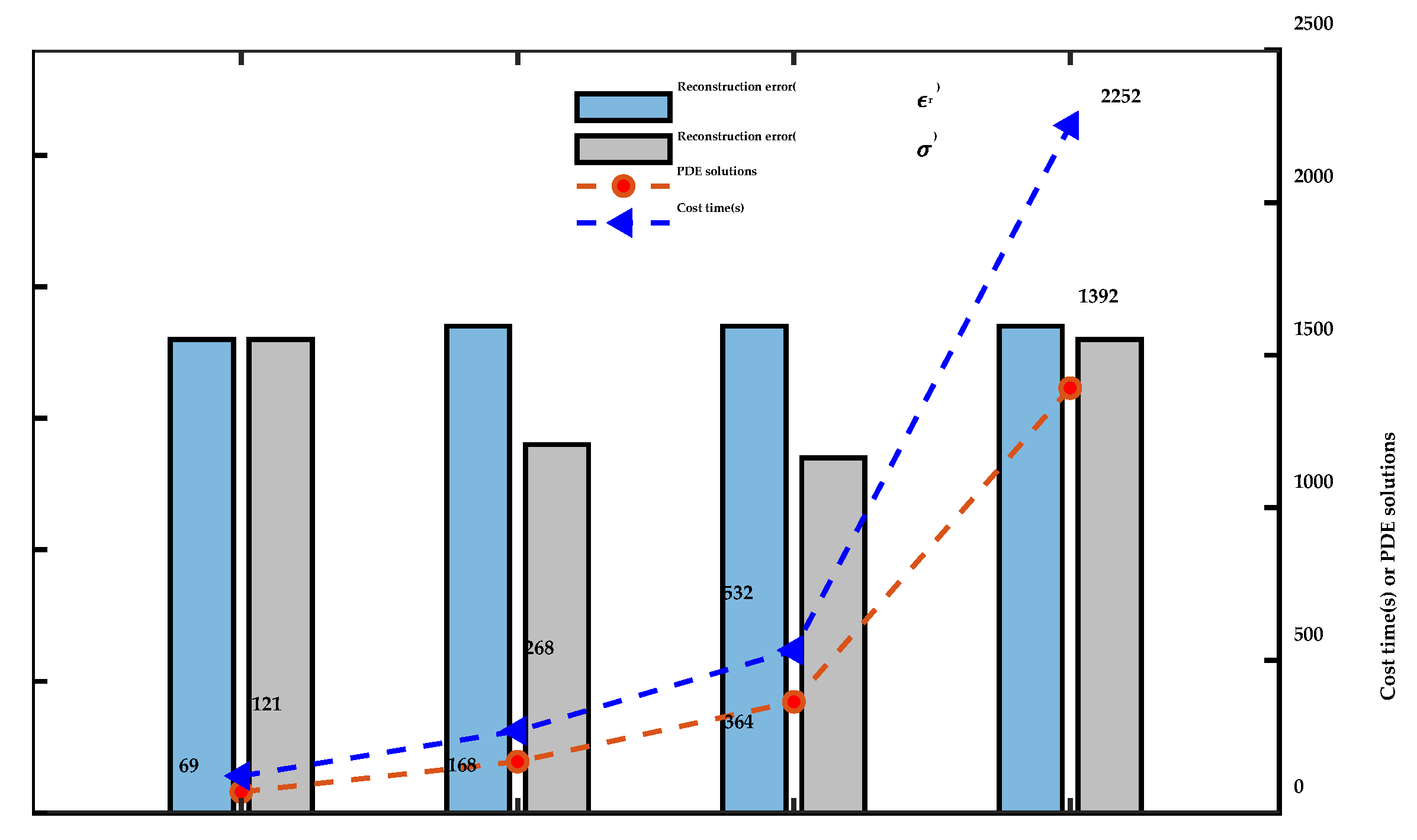
• We applied WRI to quantitatively evaluate the health condition of tree trunks. In the proposed algorithm, the grouped multi-frequency strategy is used to avoid cycle skipping, and a variation projection is applied to make WRI computationally tractable.
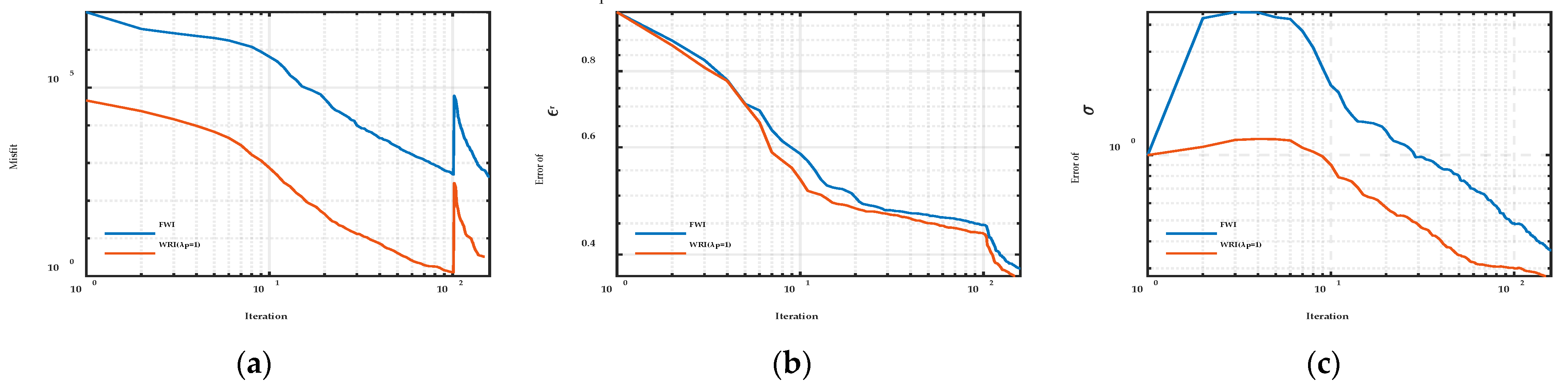
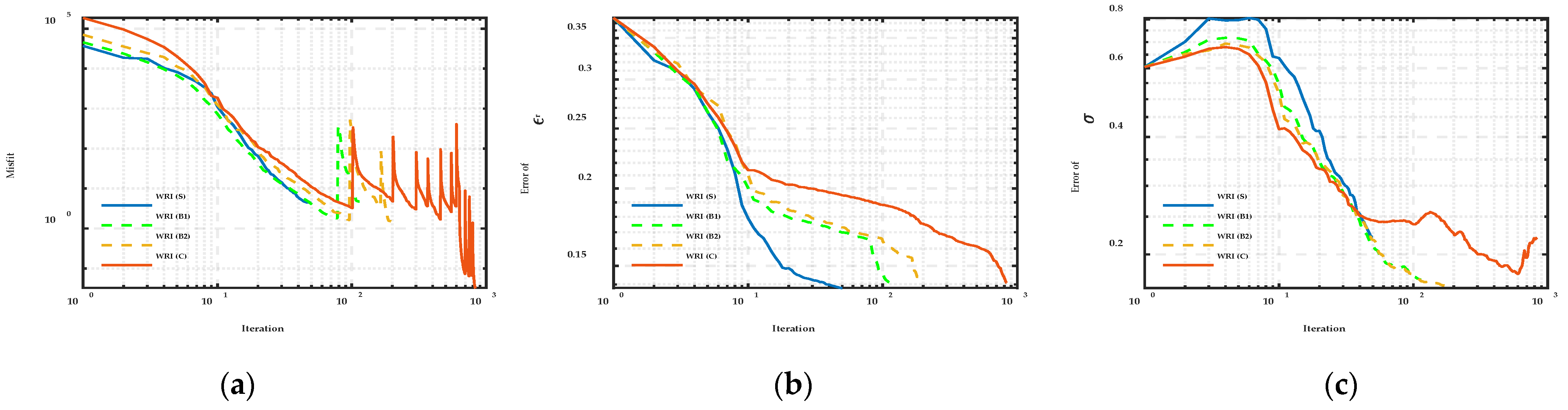
• Comparing the performance of traditional FWI and WRI under different conditions in detail. The results indicate that in contrast with traditional FWI, WRI can reduce nonlinearity and dependence on the initial model. In addition, appropriate frequency strategy and mesh generation method are important for reasonable WRI results.
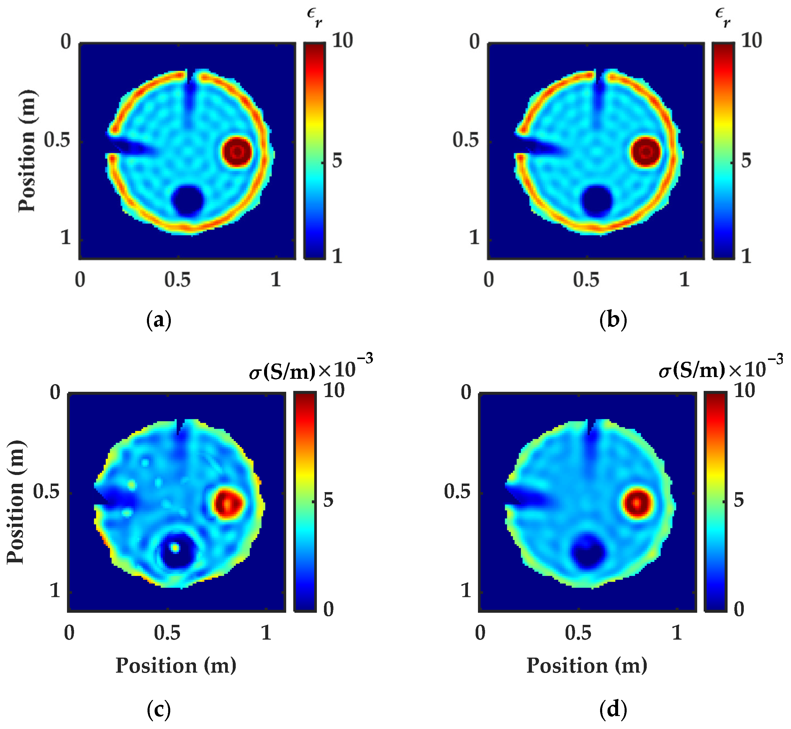
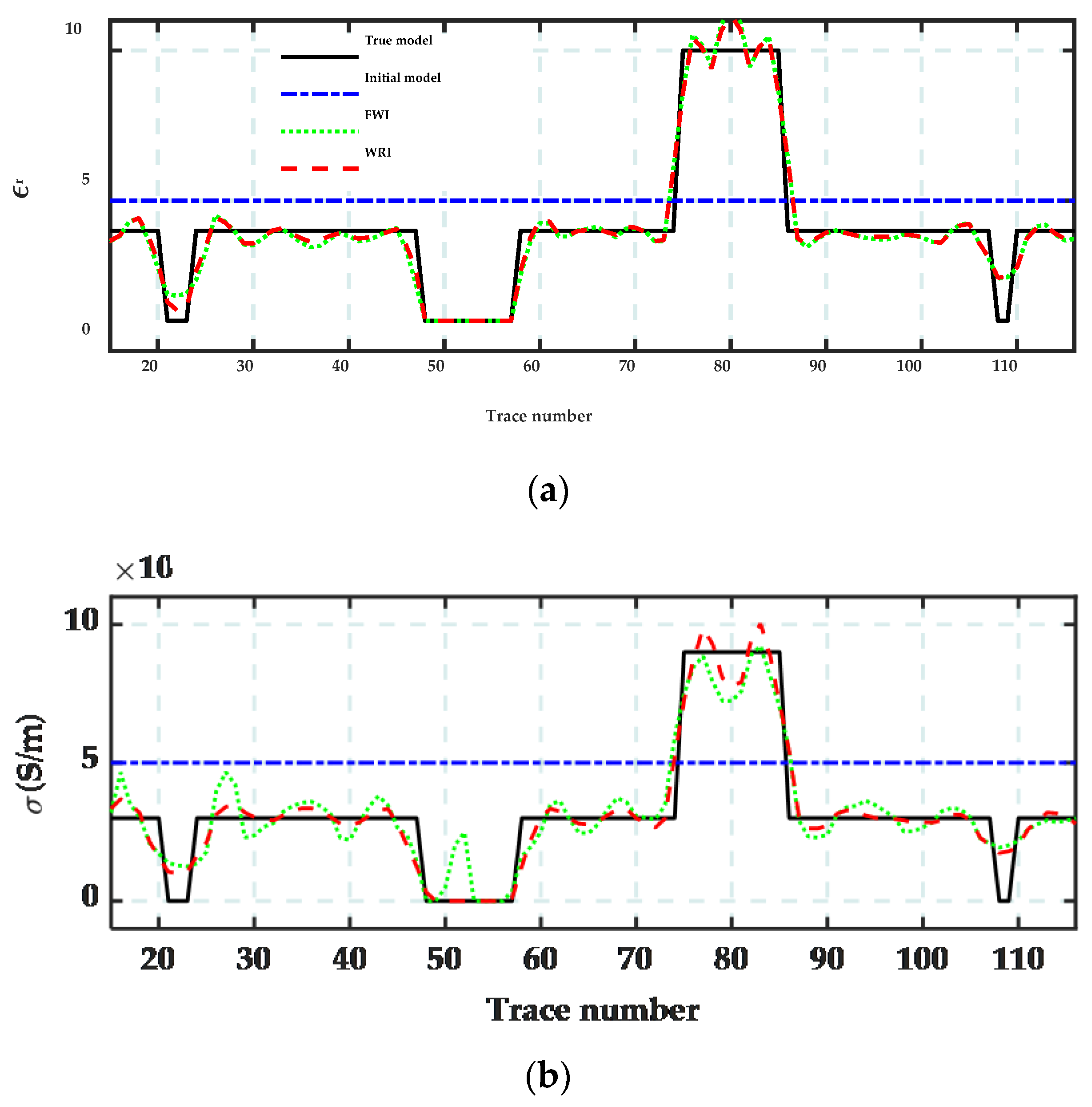
• To address the deficiency that most methods can only locate defects, the proposed WRI can accurately depict the shape, location, and properties of internal defects and structures in tree trunks. The potential of WRI in tree detection was explored through numerical and field cases. The successful results indicate that WRI has prospects in tree trunk detection.

2. Theoretical Background

Different from conventional GPR detection, tree trunk detection uses GPR to detect along the outer barks of tree trunks as shown in Figure 1a, which makes the distortion of the reflection a hyperbolic shape [36]. It indicates that low-quality GPR data caused by irregular trunk shape and source dislocation should be taken into account. According to the electromagnetic wave propagation theory, the radar wave will reflect or refract at the discontinuous electrical parameter interfaces [37]. In Figure 1b, the black solid curve, the black dotted curve, and the white solid curve represent the GPR emission wave, the echo from the opposite side of the tree trunk, and the echo from the hollow, respectively. By analyzing the echo signal, we can reconstruct the dielectric constant and conductivity of trunks and give a quantitative assessment.

To conduct the detection, Figure 2 shows the flow chart of our method, mainly including the forward simulation, the wavefield reconstruction, the gradient calculation, and the model update.

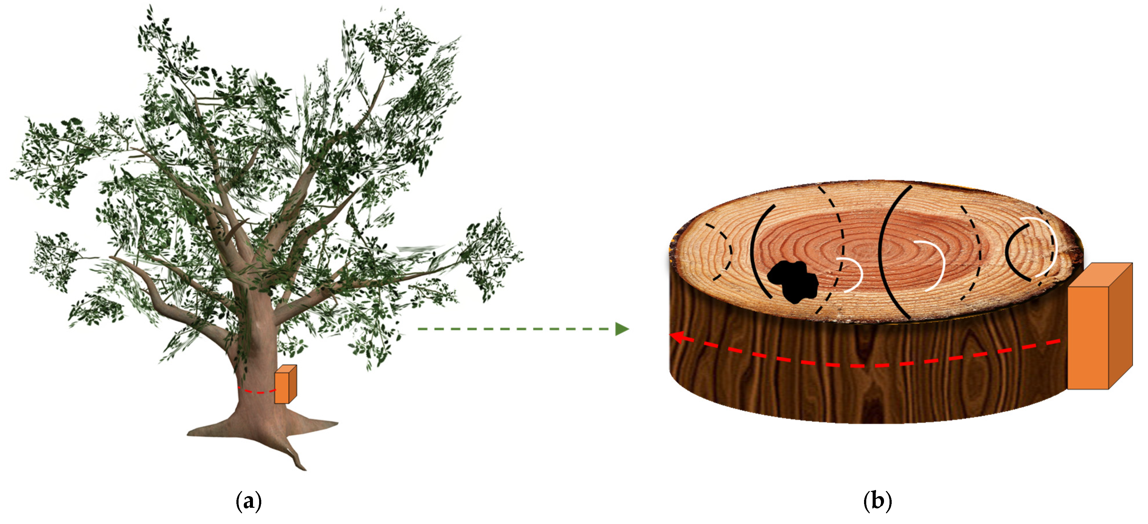
2.1. GPR Finite-Element Frequency Domain Simulation

Maxwell’s equations of 2D transverse magnetic (TM) mode in the frequency domain can be expressed by [38] the following:

$$\frac{\partial }{\partial x}\left({\alpha }_x\frac{\partial u}{\partial x}\right)+\frac{\partial }{\partial y}\left({\alpha }_y\frac{\partial u}{\partial y}\right)+\beta k^{2}u=i\omega \mu J_z,$$

(1)

where u (V/m) and J_z (A/m²) are the electric field density and current density in the frequency domain, respectively. α_x, α_y, β are anisotropic medium parameters, k = sqrt(ꞷ²εμ-iꞷσμ) is wavenumber in the frequency domain, ꞷ and I = sqrt(−1) represents the angular frequency and the imaginary unit, respectively. The model parameters ε (F/m), σ (S/m), and μ (H/m) are the dielectric constant, conductivity, and permeability of the tree trunk, respectively. In this paper, we assume that the permeability is constant.

After discretization by the finite-element frequency domain (FEFD) method, Equation (1) can be rewritten in matrix form as follows:

$$A\left(\omega ,\epsilon ,\sigma \right)u\left(\omega \right)=q\left(\omega \right),$$

(2)

where A(ꞷ,ε,σ) is the Helmholtz operator which represents a series of partial differential equations (PDEs), and u(ꞷ) and q(ꞷ) represent the wavefield vector and source vector, respectively. For the sake of simplicity, we will abbreviate A(ꞷ,ε,σ), u(ꞷ), and q(ꞷ) as A(ε,σ), u and q. Considering the irregular bark, the FEFD based on perfectly matching layers (PML) is adopted to discrete the model space and conduct the forward simulation [39].

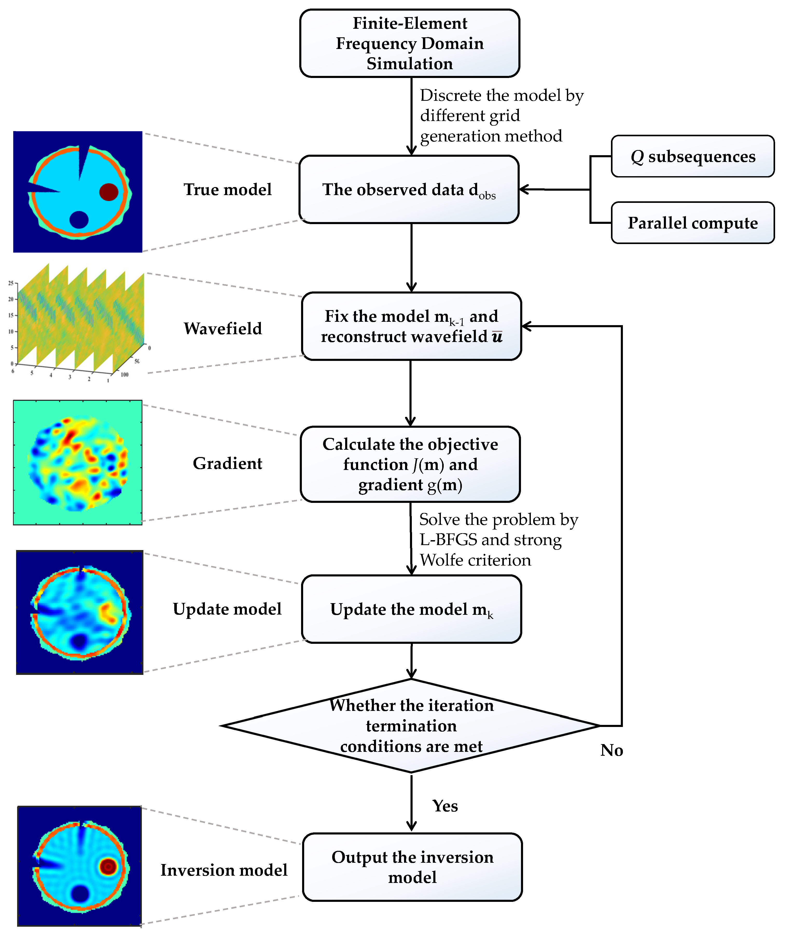
2.2. GPR-WRI in the Frequency Domain

Before introducing the WRI to the inverse problem for GPR, it is necessary to have a brief review of the conventional FWI. It can be written as a PDE-constrained optimization problem only regarding model parameters, and has the ability to reconstruct the dielectric constant and conductivity of trunks by minimizing the difference between the modeled data and the observed data:

$$\underset{m}{\min }\frac{1}{2}{\Vert PA{(m)}^{-1}q-d\Vert }_2^2,$$

(3)

where m = [m₁,m₂,…,m_M]^T represents the model parameters (containing the dielectric constant ε and conductivity σ) at each element of the finite-element mesh. M is two times the number of elements. Here, the bound constraints are considered in the inversion. The dielectric constant models are bounded by the lower bound 1 and the upper bound 81, and the conductivity models are bounded by the lower bound 0. P is an operator that extracts the modeled wavefield at the receiver positions, and d is the observed data at the same receiver. The objective function above is an optimization problem constrained by the wave equation (Equation (2)). It indicates A(m)⁻¹q is subject to Equation (2) and represents the modeled wavefield u in Equation (3).

Different from FWI constrained by the wave equation, WRI adds the wave equation term as a penalty term to the objective function. In this case, the optimization problem can be written as follows:

$$\underset{u,m}{\min }\frac{1}{2}{\Vert Pu-d\Vert }_2^2+\frac{1}{2}{\lambda }_p{\Vert A(m)u-q\Vert }_2^2,$$

(4)

where λ_p is the positive penalty parameter. The first term is the data misfit, and the second is the wave equation term. Because WRI with a small penalty parameter will become the optimized problem in weakly constrained, it has the ability to reduce the nonlinearity and dependence on the initial model [31,40].

In our previous work about WRI [33], we found that the penalty term plays an important role in adjusting the scale of the data misfit and the wave equation term. If λ_p increases, the wave equation term is more tightly constrained, and WRI is close to the conventional FWI. If λ_p decreases, the inversion will expand the search space in loose constraints by the wave equation [41].

The objective function can be described in detail as follows:

$$\begin{array}{c}\mathrm{\Phi }\left(u,m\right)=\frac{1}{2}{\displaystyle \sum _{i=1}^{N_{\omega }}{\displaystyle \sum _{j=1}^{N_s}{\left(P{u}_{i,j}-d_{i,j}\right)}^{†}\left(P{u}_{i,j}-d_{i,j}\right)}}\hfill \\ \hspace{1em}\hspace{1em}\hspace{1em} +\frac{1}{2}{\lambda }_p{\displaystyle \sum _{i=1}^{N_{\omega }}{\displaystyle \sum _{j=1}^{N_s}{\left(A_{i,j}\left(m\right)u_{i,j}-q_{i,j}\right)}^{†}\left(A_{i,j}\left(m\right)u_{i,j}-q_{i,j}\right)}}\end{array}$$

(5)

where † is the transpose-conjugate operator, and N_ω and N_s represent the number of frequency and source, respectively.

In the WRI problem, the estimation of the wavefield can be reconstructed through a variation projection method. The reconstructed wavefield approximately satisfies the wave equation and the data fit simultaneously. It can be computed efficiently with a closed-form solution:

$$\overline{u}\left(m\right)={\left({\lambda }_{p}A{\left(m\right)}^{†}A\left(m\right)+P^{T}P\right)}^{-1}\left({\lambda }_{p}A{\left(m\right)}^{†}q+P^{T}d\right),$$

(6)

where $\overline{u}$ is the reconstructed wavefields vector. Then, fixing the wavefield $\overline{u}$, we have the following misfit of a new optimization problem for updating m:

$$\begin{array}{l}J\left(m\right)=\frac{1}{2}{\displaystyle \sum _{i=1}^{N_{\omega }}{\displaystyle \sum _{j=1}^{N_s}{\left(P{\overline{u}}_{i,j}\left(m\right)-d_{i,j}\right)}^{†}\left(P{\overline{u}}_{i,j}\left(m\right)-d_{i,j}\right)}}\\ +\frac{1}{2}{\lambda }_p{\displaystyle \sum _{i=1}^{N_{\omega }}{\displaystyle \sum _{j=1}^{N_s}{\left(A_{i,j}\left(m\right){\overline{u}}_{i,j}\left(m\right)-q_{i,j}\right)}^{†}\left(A_{i,j}\left(m\right){\overline{u}}_{i,j}\left(m\right)-q_{i,j}\right)}}\end{array}$$

(7)

We can update the model parameters as what is performed in conventional FWI (adjoint state method). Hence, with the fixed wavefields, the expression of the gradient is given by the following:

$$\mathrm{g}\left(m\right)=\nabla J\left(m\right)={\displaystyle \sum _{i=1}^{N_{\omega }}{\displaystyle \sum _{j=1}^{N_s}\Re \left\{{\lambda }_p{\overline{u}}_{i,j}^{†}{G}_{i,j}^{†}\left(A_{i,j}\left(m\right){\overline{u}}_{i,j}-q_{i,j}\right)\right\}}},$$

(8)

where $\Re$ is the real part operator, and G = ∂A(m)/∂m is the diffraction matrix. In this paper, we update the optimization problem via the limited-memory Broyden–Fletcher–Goldfarb–Shanno algorithm (L-BFGS) algorithm [42].

2.3. The Grouped Multi-Frequency Strategy

Different frequencies of GPR data contain different scale structural information. The low-frequency component can describe large-scale features, but cannot depict the details of features smaller than the wavelength of radar waves. While the high-frequency component has the ability to reconstruct the details, it easily leads to inversion failure caused by complex electromagnetic and strong nonlinearity. Therefore, combining the low-frequency component and high-frequency component contributes to the higher precise reconstruction of tree trunks [29,43].

In this paper, we conduct multi-frequency inversion to avoid cycle skipping. Firstly, we should select the appropriate frequency component from the original GPR data as the total inversion frequency sequence F = (ꞷ₁, ꞷ₂, …, ꞷ_i, …, ꞷ_Nꞷ). Then, sorting the data from low-frequency to high-frequency, and dividing the sorted data into Q subsequences. Each subsequent C_i (i = 1, 2, …, Q) is a subset of the total inversion frequency sequence. Next, the first subsequence on the initial model until the iteration termination condition is inverted, and the inversion resulting model at the previous subsequence is used as the new initial model of the next subsequence. In detail, the frequency component of each subsequence can be described as follows:

$$\stackrel{C_1}{\overbrace{{\omega }_1,\cdots ,{\omega }_U},}\stackrel{C_2}{\overbrace{{\omega }_{U+1},\cdots ,{\omega }_{2*U}},}\cdots ,\stackrel{C_{Q-1}}{\overbrace{{\omega }_{(Q-2)*U+1},\cdots ,{\omega }_{(Q-1)*U}},}\stackrel{C_Q}{\overbrace{{\omega }_{(Q-1)*U+1},\cdots ,{\omega }_{N_w}}},$$

(9)

where U = ceil(Nꞷ/Q) represents the number of the frequency component in each subsequence, and ceil is a round-up function.

3. Numerical Examples

To evaluate the advantages of WRI over FWI and verify the effectiveness of WRI on the parameter reconstruction for tree trunks, several numerical cases are used to investigate the influence of the penalty parameter, initial model, multi-frequency strategy, and grid generation method on WRI and compare with the conventional FWI. We adopt the regular quadrilateral simulation grid to discrete the forward simulation space, and the dimensions of the space are 1.1 × 1.1 m (including PML) with a grid interval of 0.01 m. To fit reality, we construct a three-layer tree trunk with an irregular shape, which is shown in Figure 3a,d. The background medium is a loaded air layer whose dielectric constant and conductivity are 1 and 0.000 S/m. The three layers are bark, cambium, and sapwood from outside to inside, whose outer diameters are 0.92 m, 0.84 m, and 0.76 m, respectively. The dielectric constants of the three layers are 5, 8, and 4, respectively. The conductivities are 0.005 S/m, 0.004 S/m, and 0.003 S/m, respectively. The true model contains three types of defects: hollow, cracks, and decay. Due to the invasion of decay-inducing bacteria, the moisture content and conductive ion concentration of decay are higher than healthy xylem. The dielectric constant and conductivity of decay are 10 and 0.009 S/m, while the electrical parameters of hollow and cracks are the same as air.

The FEFD method is used to generate synthetic data. We locate 23 transmitters and 115 receivers around the model evenly, which is 0.05 m from the bark. The red circles “○” and green forks “×” in Figure 3 represent the transmitting antennas and receiving antennas, respectively. The white dotted curve at a radius of 0.28 m is the profile for inversion comparison. For each transmitting antenna, the GPR signal is recorded by all the receivers. The source signature is Ricker wavelet with a center frequency of 900 MHz. The 12 frequency components (550, 575, 600, 625, 650, 675, 700, 750, 800, 850, 900, and 950 MHz) are combined as the total inversion frequency sequence. For the multi-frequency strategy, the data is grouped into Q subsequences to be inverted in order. Therefore, if Q = 2, the total frequency sequence is divided into two subsets, C₁ (550, 575, 600, 625, 650, 675 MHz) and C₂ (700, 750, 800, 850, 900, 950 MHz). We set a misfit of Φ⁽⁰⁾/Φ^(k) ≤ 1 × 10⁻⁵ or the maximum iterations in each frequency subsequence as the iteration termination condition. Specifically, each frequency subsequence maximum iteration is set as 100.

The reconstruction error is used to quantitatively assess the performance of inversion, which is denoted as follows:

$$\mathrm{Error}={\Vert m_{\mathrm{true}}-m_{\mathrm{inv}}\Vert }_2^2/{\Vert m_{\mathrm{true}}\Vert }_2^2,$$

(10)

where m_true and m_inv denote the true model and the inverted model.

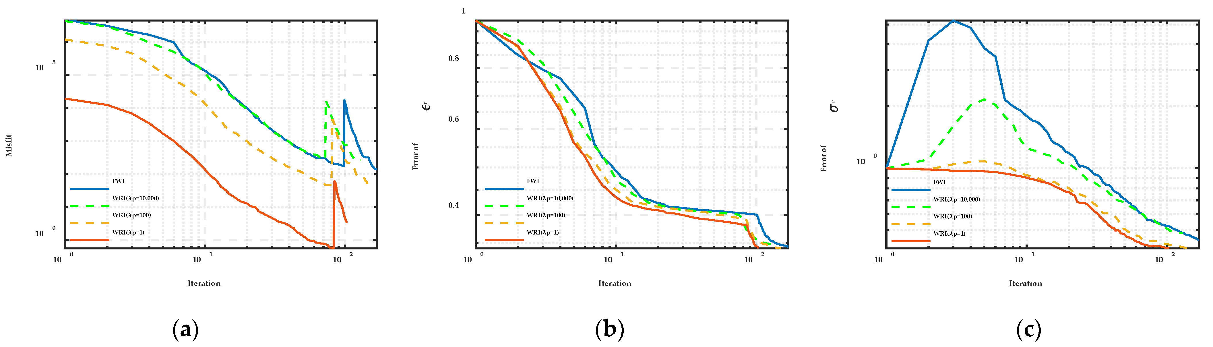
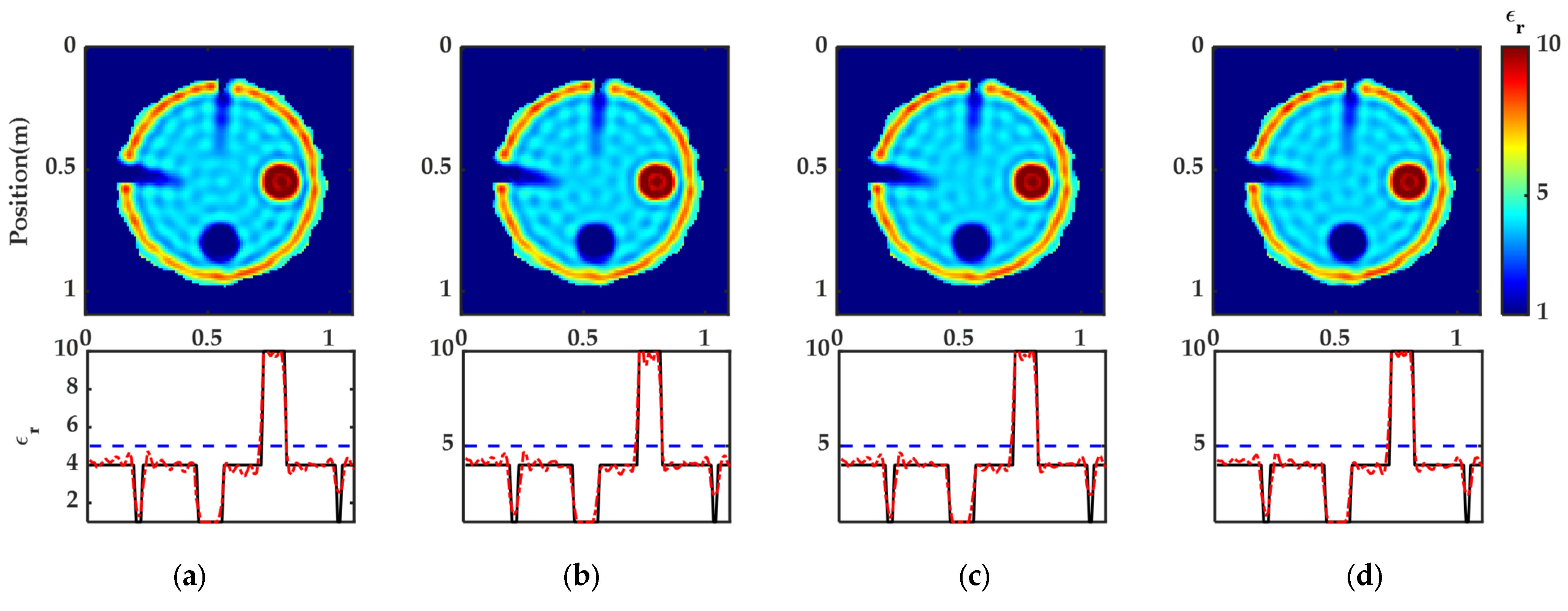
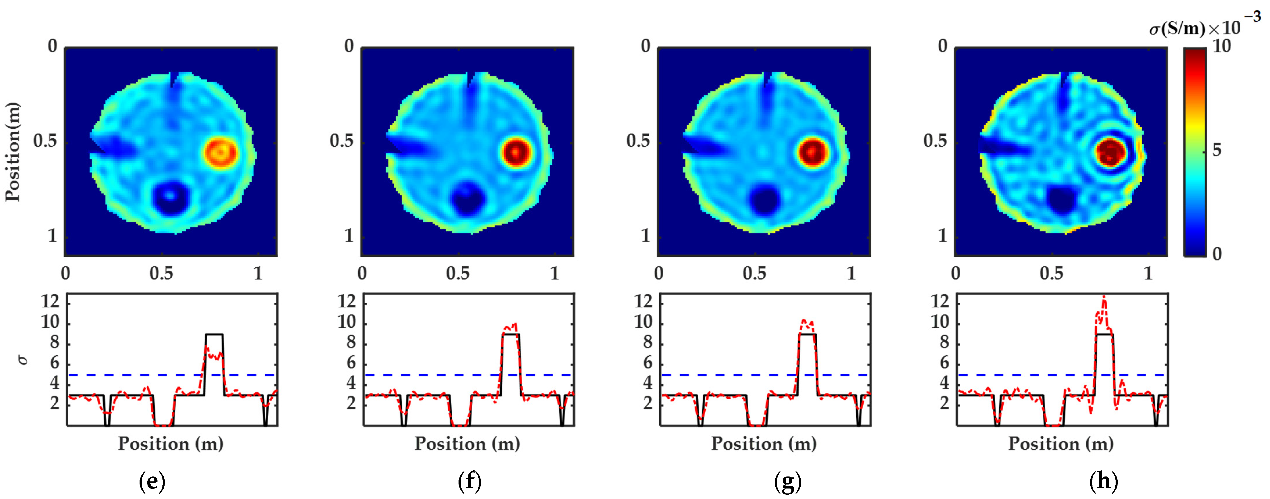
3.1. Effect of the Penalty Parameter

WRI adds the wave equation to the objective function by penalty parameter to mitigate the nonlinearity and dependence on the initial model. Therefore, the selection of the penalty parameter is crucial to the inversion success. To discuss the effect of the penalty parameter, this case compares the reconstructed models of FWI and WRI with different penalty parameters. The three-layer uniform model (as shown in Figure 3b,e), whose layer types are the same as the true model, is set as the initial model at the first subsequence. The initial model without hollow and decay simulates the unknown internal information in detection. For short, this initial model is written as IM1. For cracks that are external defects, the initial model shows only the position of the cracks without depth or other details.

In this section, three representative penalty parameters for WRI are tested as follows: λ_p = 1, λ_p = 100, and λ_p = 10,000. The total inversion frequency sequence is subsampled to two subsequences (Q = 2) to conduct inversion. Figure 4 shows the inversion results and detailed profile of FWI and WRI with three different penalty parameters. Below each figure is the detailed profile for the while dotted curve in Figure 3a,b, where black, blue, and red curves represent the parameter value from the true, initial, and reconstructed models, respectively. Figure 4a–d are reconstructed models of the dielectric constant, which are in accordance with the true model shown in Figure 3a,b. From the results, we can obtain the location, size, and shape of internal defects. Some details such as the crack depth and the cambium width are depicted well. Additionally, the specific value fits well with the true value in the profile. It indicates that FWI and WRI both have the potential to describe the dielectric constant of tree trunks. Figure 4e–h are the conductivity results and have a lower resolution than the dielectric constant results. Additionally, the comparisons of FWI and WRI are visible. For the FWI result, the shape of the hollow occurs distortion and the disturbances hinder the identification of defects and structure. WRI with larger λ_p mitigates the disturbances and artifacts, but the conductivity value of decay is a little different from the true model. From the results shown in Figure 4, as the penalty parameter λ_p decreases, the reconstructed model is closer to the true model and the disturbance mitigates obviously.

To quantitatively assess the effect of the penalty parameter on WRI and the difference between FWI and WRI, Figure 5 shows the reconstruction errors, PDE solutions, and cost time. The bar chart illustrates that there is no significant difference in accuracy between FWI and WRI. However, under similar accuracy, PDE solutions and cost time of FWI are larger than WRI regardless of the selection of λ_p. Moreover, as λ_p decreases, equation solutions and time reduce continuously.

In Figure 6a, the misfits under different inversion methods during the iteration processes are plotted. It should be noticed that the red curve (represent WRI with λ_p = 1) has less misfit and terminates iteration fastest. While in Figure 6b,c, they show the comparison of model reconstruction error convergence curves under different inversion methods. Regardless of dielectric constant and conductivity, WRI with λ_p = 1 or λ_p = 100 appears with smaller final errors and numbers of iterations. In Figure 6c, what is interesting is that the blue and green curves (represent FWI and WRI with λ_p = 10,000) first rise and then fall. The possible reason is that they have stronger nonlinearity and dependence on the initial model. The continuous decline of the red curve proves that WRI with a small penalty parameter can reduce the nonlinearity and dependence on the initial model.

This case shows that the inversion results by WRI will be similar to FWI with λ_p increases, which is consistent with the principle. As λ_p decreases, the resolution and efficiency of WRI increase. Specifically, when λ_p = 1 in this model, the cost time used WRI is reduced to one-half of the cost time used FWI. Furthermore, the PDE solutions used WRI are reduced to one-third of the PDE solutions used FWI, which means WRI greatly improves computational efficiency. The improvement indicates that WRI has promising potential to detect trunk defects efficiently and delicately.

3.2. Effect of the Initial Model

Limited by detection cost and tree individual difference, the prior information of each tree trunk is difficult to acquire in large-scale tree trunk detection, causing an appropriate initial model hard to construct. To test the effect of the initial model on FWI and WRI, the homogeneous model (as shown in Figure 3c,f) is set as the initial model whose dielectric constant and conductivity are 5 and 0.005 S/m, respectively. The inaccurate initial model will be written as IM2 later for short. In this case, the total inversion frequency sequence is subsampled to two subsequences (Q = 2) to conduct inversion and the penalty parameter λ_p = 1.

Figure 7 illustrates the reconstructed model of dielectric constant and conductivity by conventional FWI and WRI with little penalty parameter on IM2. There is no doubt that the precision and resolution of the results in Figure 4 are generally superior to this case, which indicates the initial model plays an important role in inversion. In dielectric constant results, although the initial model is far from the true model, both FWI and WRI have captured three-layer structure and internal defects. The conductivity result of FWI cannot describe the accurate boundary, whereas WRI can depict the accurate structure and defects with lower disturbance. Additionally, for cracks that are slender type defects, the conductivity resolution of FWI is inferior to WRI, and FWI cannot obtain the growth space and extension direction.

To further analyze the subtle influence of the initial model on WRI and FWI, Figure 8 shows profiles of dielectric constant and conductivity, where black, blue, green, and red curves represent the specific parameter value from the true, initial, FWI resulting, and WRI resulting models. In Figure 8a, the knee points and extremum of the green and red curve fit well with the black curve, which indicates both FWI and WRI can describe the distribution of the dielectric constant of trunks. Figure 8b shows that the conductivity curve of WRI fits better than FWI, especially for hollow. Additionally, the PDE solutions and cost time of FWI and WRI are 190 and 268 s and 168 and 203 s, respectively.

In Figure 9, the convergence curve of misfit and model reconstruction error during the iteration processes are plotted. WRI with λ_p = 1 appears with the smallest final error and number of iterations in Figure 9a–c.

This case indicates that the initial model plays a crucial role in inversion. The inaccurate initial model will reduce the precision and make inversion fall in the informative local minimum easily. However, WRI with a small penalty parameter can still image the structure of tree trunks in the lack of an accurate initial model. Additionally, WRI decreases the cost time and the PDE solutions in this case. Therefore, in contrast with FWI, WRI has better applicability and robustness when the initial model is not accurate.

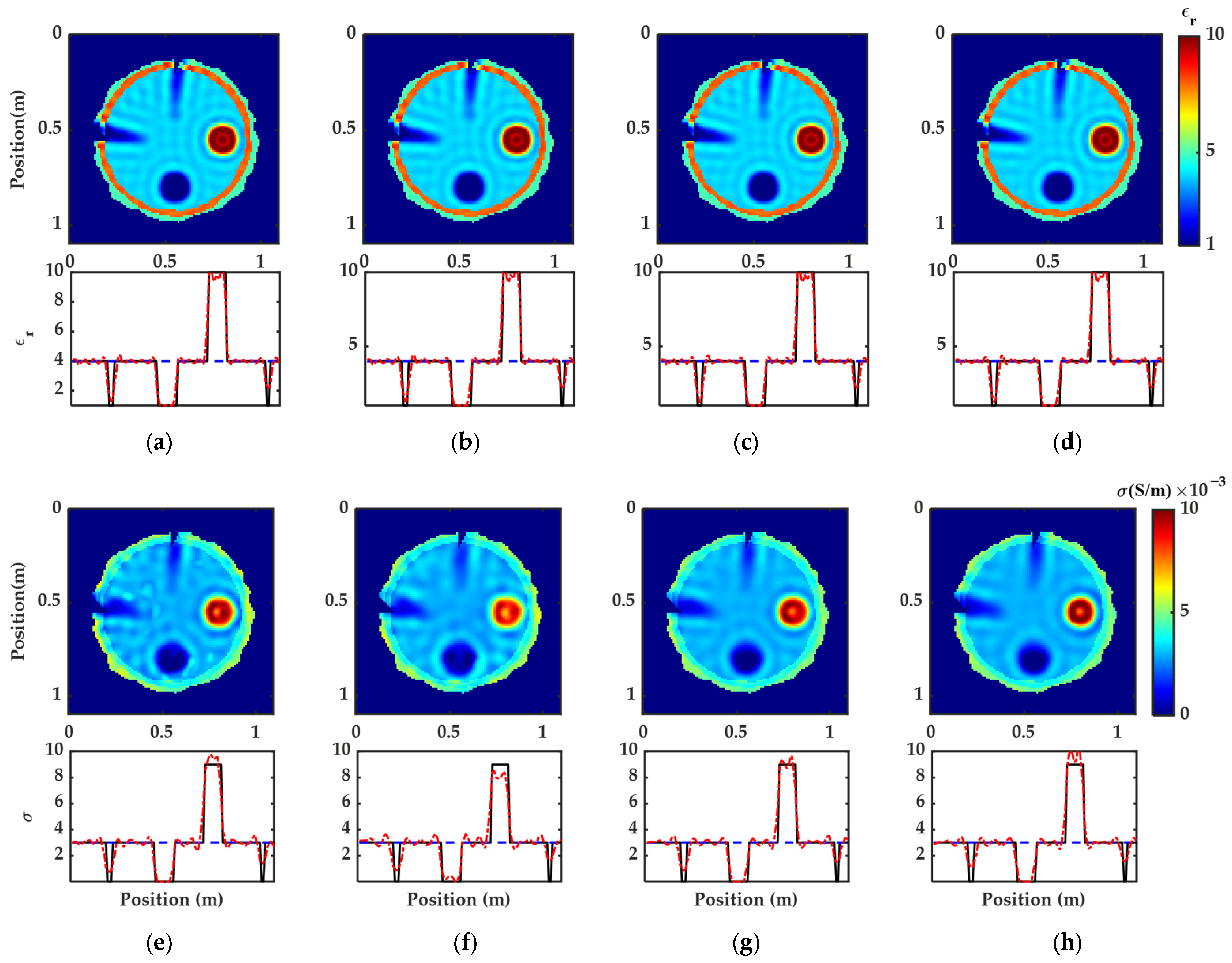
3.3. Effect of the Frequency Strategy

In this case, we set IM2 as the initial model (as shown in Figure 3c,f). Twelve frequency components (550, 575, 600, 625, 650, 675, 700, 750, 800, 850, 900, and 950 MHz) are combined as the total inversion frequency sequence. To prove the advantages of the proposed frequency strategy over the former strategies, we compare the inversion results by different frequency strategies: (1) simultaneous multi-frequency strategy (twelve frequency components are inverted simultaneously, and called briefly by S strategy); (2) grouped multi-frequency strategy (subsampling twelve frequency components into Q = 2 subsequence to inversion in order, and called briefly by B1 strategy); (3) grouped multi-frequency strategy (subsampling twelve frequency components into Q = 3 subsequence to inversion in order, and called briefly by B2 strategy); (4) sequential strategy (each frequency component is inverted in order, and called briefly by C strategy). The penalty parameter λ_p = 1.

Figure 10 shows the inversion results of WRI using different frequency strategies. In general, the inversion results of the dielectric constant are superior to conductivity. Additionally, B1 and B2 strategies are significantly better than S and C strategies, especially for conductivity. The conductivity result of WRI with S strategy (as shown in Figure 10e) has a lower resolution than other strategies. Additionally, the boundary of cracks is blurred, so it is hard to obtain the depth and shape of cracks. As for C strategy in Figure 10f, although the resolution improves, the oscillation and artifacts become more serious. Even the shape of hollow is distorted. A possible reason is that in the later iteration of C strategy, there are only high-frequency data, which is conducive to small-sized feature reconstruction, but also brings disturbance, hindering the capture of defects and structure. In comparing profiles, there is a larger deviation in the conductivity value of WRI with S and C strategies. The proposed multi-frequency strategy B1 and B2 perform better, which indicates combining different frequency components and sequential inversion is a desirable strategy to stabilize the inversion and improve the resolution.

Figure 11 compares the reconstruction error, PDE solutions, and cost time of different frequency strategies. The bar chart shows that the reconstruction errors of S strategy are the largest, and those of the proposed B strategy are relatively small. Additionally, the line chart indicates that as the number of subsequences increases, PDE solutions and cost time increase continuously. Thus, the cost time of C strategy is 2252 s, which is not a practical strategy in tree trunk detection. Specifically, at the expense of reducing the reconstruction error, the cost time of B1 and B2 are 1.2 and 3.4 multiples of S.

In Figure 12a, the misfits under WRI with different frequency strategies on IM2 during the iteration processes are plotted. The trends are similar to the former case shown in Figure 6a. In the error convergence curves of the dielectric constant shown in Figure 12b, the end number of iteration of S < B1 < B2 < C, while the convergence errors are similar, which corresponds with the blue bar chart in Figure 11. In the error convergence curves of conductivity shown in Figure 12c, strategies B1 and B2 show the small final error and the slightly increased number of iterations at the end of the optimization.

Therefore, the proposed multi-frequency strategy can improve the inversion accuracy and resolution with acceptable computational efficiency loss, which is a desirable strategy in actual detection.

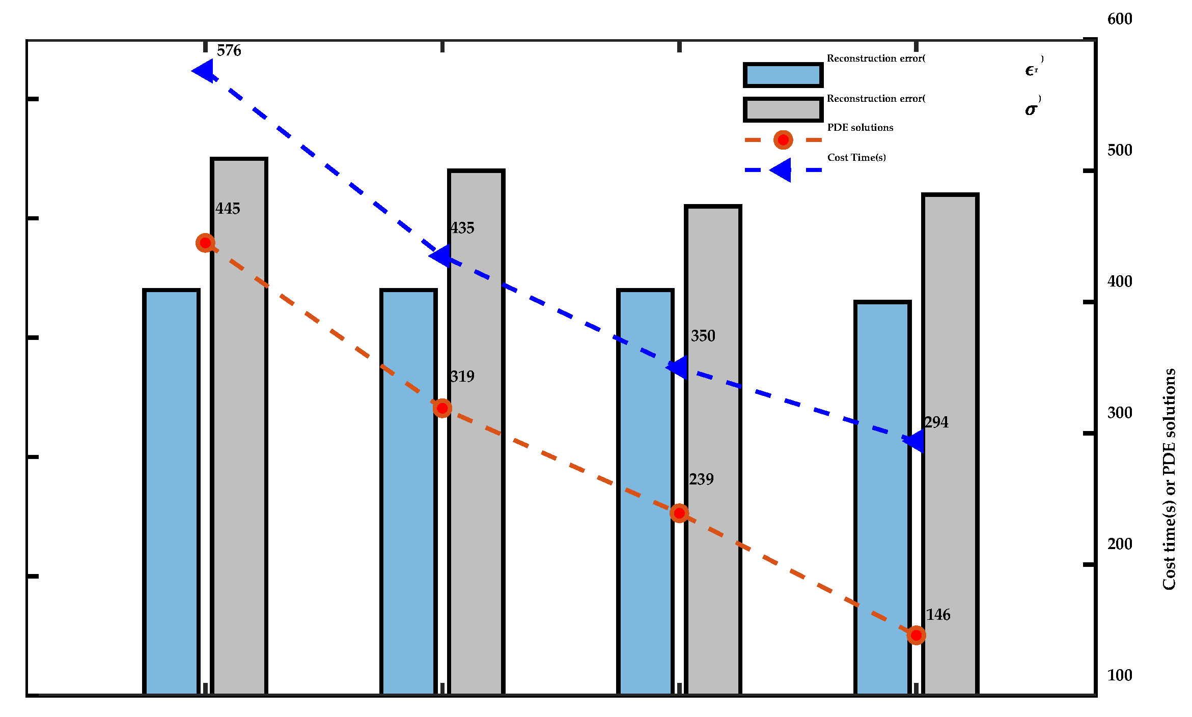
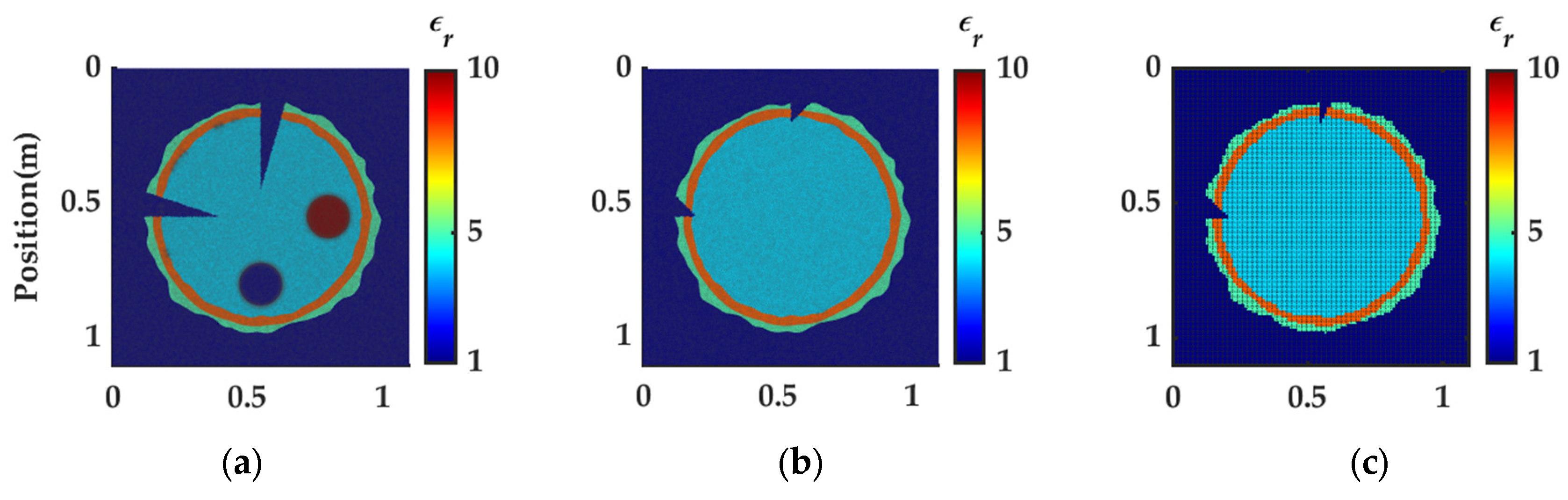
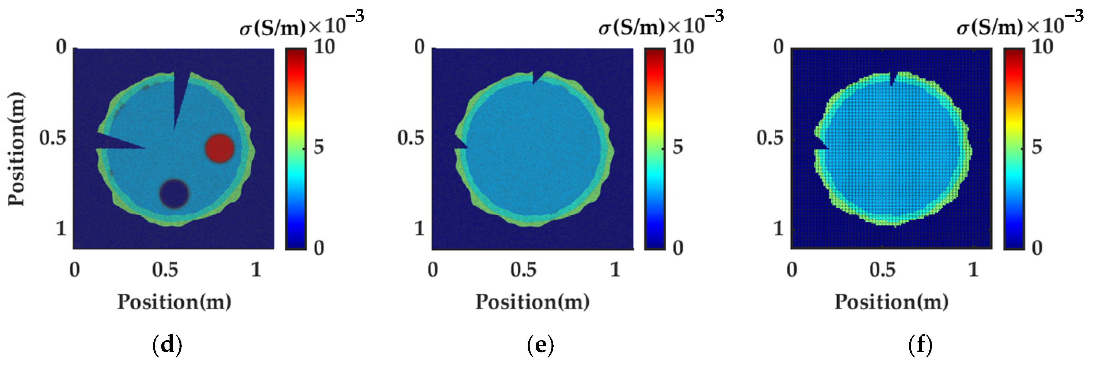
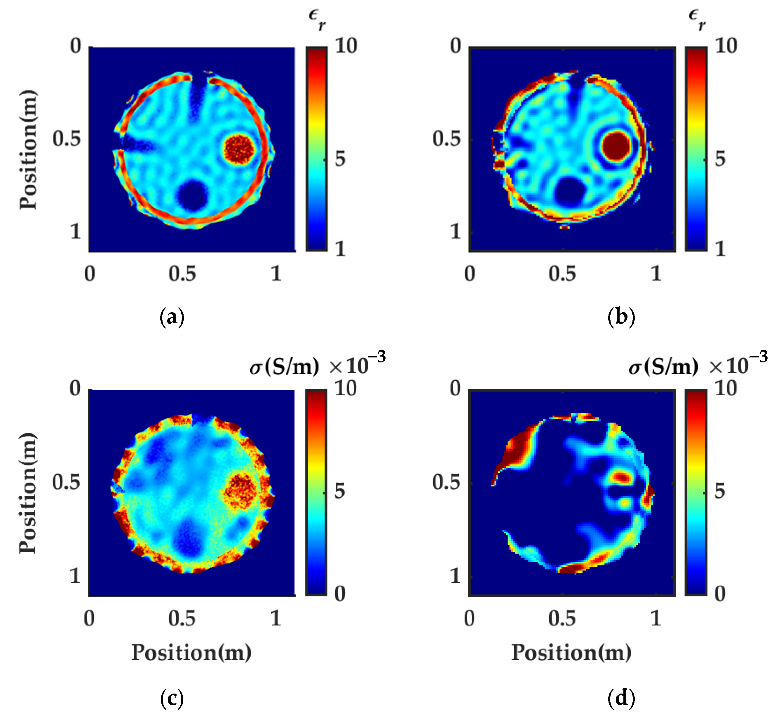
3.4. Effect of the Grid Generation Method

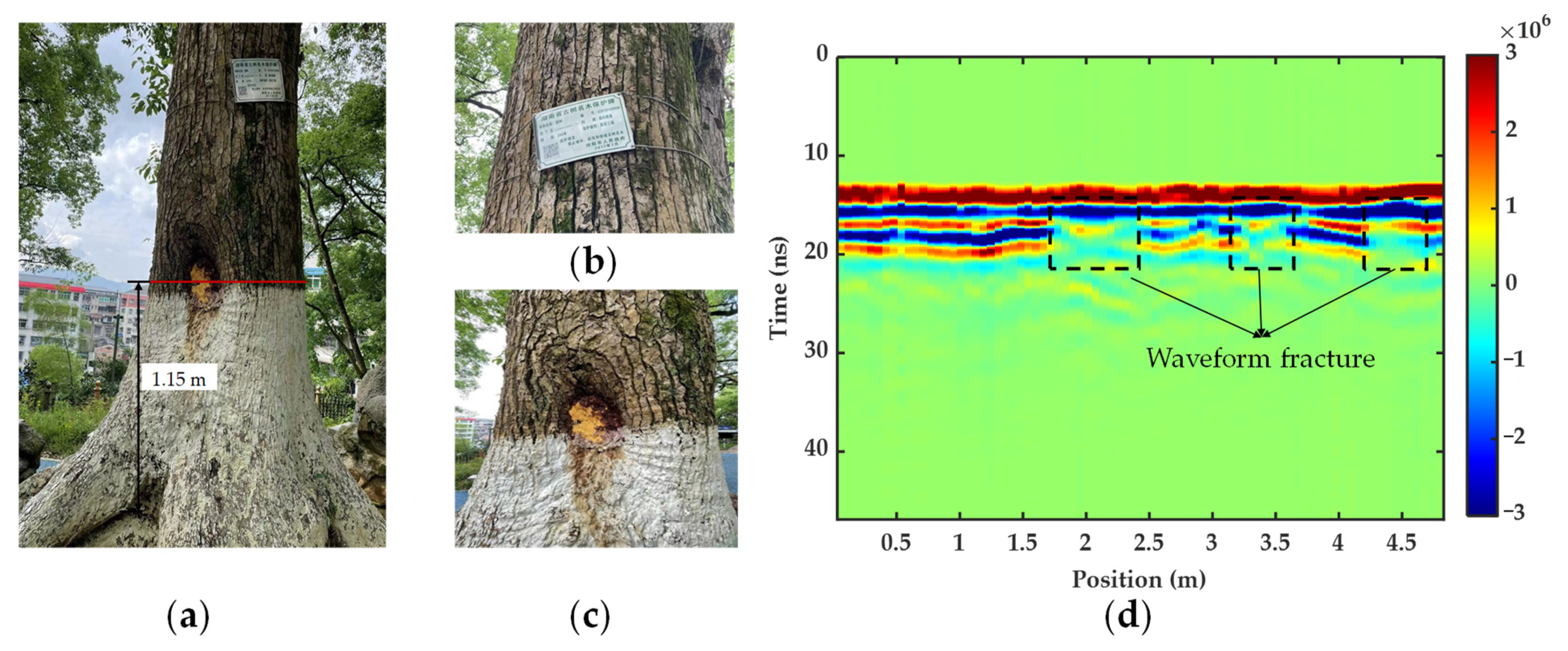
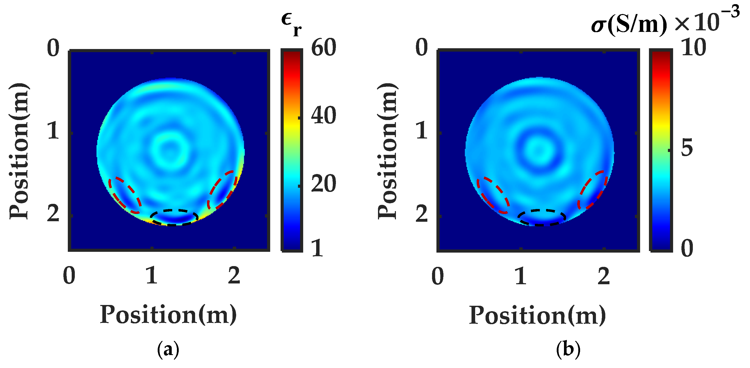
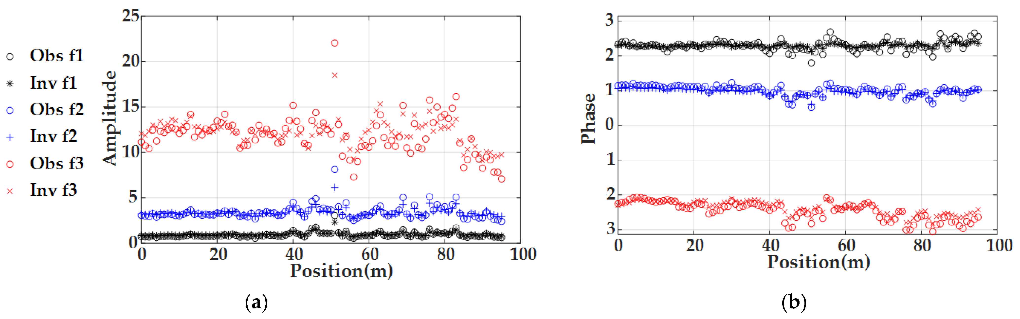
The above synthetic cases have verified the validity and advantages of WRI based on regular quadrilateral mesh in tree trunk detection. However, the mesh cannot simulate the uneven bark perfectly. Therefore, this case discusses the effect of two different grid generation methods (including irregular triangular mesh and regular quadrilateral mesh) on WRI.

We adopt FEFD based on the irregular triangular mesh to discrete simulation space and generate synthetic GPR data. Figure 13 shows the true model and the initial model discretized by different grid generation methods, and the specific grid distribution is overlaid on the model diagram to display. The true models are shown in Figure 13a,d. the numbers of nodes and elements are 78,539 and 156,324, respectively. Obviously, the model is discretized by the irregular triangular mesh, which is smoother than regular quadrilateral mesh (as shown in Figure 3a,d). Therefore, the irregular triangular mesh fits reality better. For the reconstructed grid, we adopt relatively sparse grids to discretize the initial model (as shown in Figure 13b,e) and reduce unnecessary calculations. The nodes and elements number of irregular triangular mesh are 48,166 and 95,730, while the grid interval of regular quadrilateral mesh is 0.01 m with a total of 12,100 elements (as shown in Figure 13c,f). B2 strategy is employed until the inversion finishes.

Figure 14a,c show the reconstruction of dielectric constant and conductivity by WRI based on irregular inversion mesh. The dielectric constant result is basically coincidental with the true model, the boundary of cracks is more clear than the result in Figure 4d, and the resolution also improves. However, the conductivity result only depicts hollow and decay without cracks. Additionally, the disturbance and near-source error are strong. A possible reason is that although the accuracy of irregular mesh is higher than regular mesh in principle, the free degree of irregular mesh is higher on the premise of the same nodes, strengthening the nonlinearity and ambiguity of WRI. Thus, sensitive conductivity result deteriorates. Through the mutual verification and restriction of dielectric constant and conductivity, we can still identify the specific type of defects and structure. Compared to Figure 14a,c, the results based on regular mesh (as shown in Figure 14b,d) cannot describe the accurate shape and location of defects. There is a large deviation from the true model, especially for conductivity.

This case indicates that the inversion with irregular mesh performs better than that with the regular mesh, especially the estimate for the conductivity. Aside from this phenomenon, we noted the failure of parametric estimation in the region around the sources. Remember, we used a complex mesh relatively closer to reality, which explains the importance of the exact source location and the accurate mesh for the inversion.

4. Field Example

A field experiment is conducted with the GPR system on a living tree in Liuyang, Hunan Province (China). As shown in Figure 15a–c, this is a camphor tree under third-level national protection. The grith of this camphor tree is approximately 4.8 m. Relevant background knowledge lets us know that there is a small area of hollow in the tree trunk which has been filled with foam. The obvious irregular outer contour of the trunk shows the position of the filled hollow, while the size and shape of the filled area are unknown. To judge the hollow subsequent recovery and further monitor the tree health condition, we use GPR to nondestructively detect the living tree. In this case, the data of the cross-section in the height of 1.15 m was measured using a 400 MHz antenna manufactured by Geophysical Survey Systems Inc. (GSSI). When acquiring data, the bottom of the radar antenna needs to be as close as possible to the trunk surface to prevent electromagnetic wave attenuation. The trace interval is 0.05 m, the total time window is 86 ns, and the number of time samples is 1024. The measurement mode adopts a point-by-point acquisition mode. Figure 15d shows the original GPR data before 50 ns which contains 96 traces. There are three waveform fractures in the original GPR data, which indicate other invisible defects that need to be maintained.

In this case, we used an irregular triangular mesh with 12,043 nodes and 23,784 elements to discrete the calculation area. There are 96 sources and receivers located in the air outer the tree trunk. The initial model of the tree trunk is a uniform medium, and its dielectric constant and conductivity are set to 20 and 0.003 S/m, respectively. Before inversion, we transformed the original data from the time domain to the frequency domain. We used the data from 0 ns to 50 ns. A total of 21 frequency components (19.8, 39.7, 59.5, 79.4, 99.2, 119.1, 138.9, 158.8, 178.6, 198.4, 218.3, 238.1, 258.0, 277.8, 297.7, 317.5, 337.4, 397.0, 416.7, 436.6, and 456.4 MHz) are used to conduct inversion. The total inversion frequency sequence is subsampled to two subsequences (Q = 3), and the penalty parameter λ_p = 1.

Figure 16a,b show the reconstruction of the dielectric constant and conductivity of the field data, in which the internal layered structure is well reconstructed. In the lower part of the model circled by the black curve, there is a region with a low dielectric constant and conductivity. This corresponds to the filled hollow of the detected tree. The filled hollow in the reconstruction result agrees well with the reality, whose depth and width are 0.16 m and 0.51 m, respectively. The coincidence indicates the success of the preliminary filled work. However, it should be noted that there are invisible internal hollows on both sides of the cavity circled by the red curve, which alert staff to additional protective work.

Figure 17a,b show the amplitudes and phases of the original observation data and the data simulated by recovered models at three frequencies (99.2 MHz, 218.3 MHz, and 416.7 MHz). The differences between these data are small, although they exist, especially in the position close to the abnormal internal defects. Additionally, compared to low-frequency data, high-frequency data have greater errors. A possible reason is that low-frequency data only have the ability to reconstruct large-scale information, while high-frequency data is more sensitive to small-scale information. Therefore, in field detection, observation factors (such as uneven bark, inaccurate radar location, etc.) will reduce the accuracy of reconstructed results using high-frequency data. In the future, point cloud technology and three-dimensional reconstruction will be the follow-up work to solve these problems. Overall, the errors in the field case are within the acceptable range, which demonstrates that the proposed algorithm performs great applicability and is conducive to monitoring the living tree health condition and checking the restoration work.

5. Conclusions

In this paper, we applied the recently proposed wavefield reconstruction dual-parameter inversion of GPR data in tree trunk detection. Compared with the conventional FWI algorithm, the proposed algorithm can better reconstruct the internal defects of tree trunks in qualitative and quantitative with a high imaging accuracy. As an imaging technique, it can be used for the detection and maintenance of living trees, as well as providing necessary data and theoretical support for rehabilitation and other work.

The effectiveness of the proposed method is verified by both simulated and field GPR data. The experimental results of an irregularly shaped three-layer tree trunk model with hollow, cracks, and decay show that we can obtain a more ideal and accurate reconstruction of the tree trunk by selecting the appropriate small penalty factor, frequency stacking strategy, and irregular triangular mesh. A realistic field example with a historic tree suggests that the proposed method can reconstruct the shapes and identify the defects of the tree trunk. However, there are still limitations in the inversion results of small structure, conductivity, and calculation efficiency. Future work will study more efficient inversion strategies to improve the performance in reconstruction accuracy and inversion efficiency. Additionally, the accurate location of the GPR antenna is also a worthy subject.

References

1. Linhares, C.S.F.; Goncalves, R.; Martins, L.M.; Knapic, S. Structural stability of urban trees using visual and instrumental techniques: A review. Forests 2021, 12, 1752. [Google Scholar] [CrossRef]
2. Tubby, K.V.; Webber, J.F. Pests and diseases threatening urban trees under a changing climate. Forestry 2010, 83, 451–459. [Google Scholar] [CrossRef]
3. Santini, A.; Ghelardini, L.; De Pace, C.; Desprez-Loustau, M.L.; Capretti, P.; Chandelier, A.; Cech, T.; Chira, D.; Diamandis, S.; Gaitniekis, T.; et al. Biogeographical patterns and determinants of invasion by forest pathogens in Europe. New Phytol. 2013, 197, 238–250. [Google Scholar] [CrossRef]
4. Guo, Q.; Rejmanek, M.; Wen, J. Geographical, socioeconomic, and ecological determinants of exotic plant naturalization in the United States: Insights and updates from improved data. NeoBiota 2012, 12, 41–55. [Google Scholar] [CrossRef]
5. Wang, X.; Allison, R.B. Decay detection in red oak trees using a combination of visual inspection, acoustic testing, and resistance microdrilling. Arboric. Urban For. 2008, 34, 1–4. [Google Scholar] [CrossRef]
6. Vossing, K.J.; Niederleithinger, E. Nondestructive assessment and imaging methods for internal inspection of timber. Holzforschung 2018, 72, 467–476. [Google Scholar] [CrossRef]
7. Van, D.D.; Laurence, S. Prediction of Static Bending Properties of Eucalyptus Clones Using Stress Wave Measurements on Standing Trees, Logs and Small Clear Specimens. Forests 2022, 13, 1728. [Google Scholar]
8. Xu, P.; Cheng, G.; Zhang, H.; Li, G.; Zhao, D.; Ross, R.J.; Shen, Y. Application of Nondestructive Testing Technologies in Preserving Historic Trees and Ancient Timber Structures in China. Forests 2021, 12, 318. [Google Scholar] [CrossRef]
9. dos Reis, M.N.; Gonçalves, R.; Brazolin, S.; de Assis Palma, S.S. Strength Loss Inference Due to Decay or Cavities in Tree Trunks Using Tomographic Imaging Data Applied to Equations Proposed in the Literature. Forests 2022, 13, 596. [Google Scholar] [CrossRef]
10. Kharrat, W.; Koubaa, A.; Khlif, M.; Bradai, C. Intra-Ring Wood Density and Dynamic Modulus of Elasticity Profiles for Black Spruce and Jack Pine from X-Ray Densitometry and Ultrasonic Wave Velocity Measurement. Forests 2019, 10, 569. [Google Scholar] [CrossRef]
11. Li, H.; Zhang, X.; Li, Z.; Wen, J.; Tan, X. A review of research on tree risk assessment methods. Forests 2022, 13, 1556. [Google Scholar] [CrossRef]
12. Liu, H.; Shi, Z.; Li, J.; Liu, C.; Meng, X.; Du, Y.; Chen, J. Detection of Cavities In Urban Cities by 3D Ground Penetrating Radar. Geophysics 2021, 86, WA25–WA33. [Google Scholar] [CrossRef]
13. Butnor, J.R.; Pruyn, M.L.; Shaw, D.C.; Harmon, M.E.; Mucciardi, A.N.; Ryan, M. Detecting defects in conifers with ground penetrating radar: Applications and challenges. For. Pathol. 2009, 39, 309–322. [Google Scholar] [CrossRef]
14. Xue, F.; Zhang, X.; Wang, Z.; Wen, J.; Guan, C.; Han, H.; Zhao, J.; Ying, N. Analysis of Imaging Internal Defects in Living Trees on Irregular Contours of Tree Trunks Using Ground-Penetrating Radar. Forests 2021, 12, 1012. [Google Scholar] [CrossRef]
15. Giannakis, I.; Tosti, F.; Lantini, L.; Alani, A.M. Health Monitoring of Tree Trunks Using Ground Penetrating Radar. IEEE Trans. Geosci. Remote Sens. 2019, 57, 8317–8326. [Google Scholar] [CrossRef]
16. Tosti, F.; Gennarelli, G.; Lantini, L.; Catapano, I.; Soldovieri, F.; Giannakis, I.; Alani, A.M. The use of GPR and microwave tomography for the assessment of the internal structure of hollow trees. IEEE Trans. Geosci. Remote Sens. 2022, 60, 1–14. [Google Scholar] [CrossRef]
17. Fedeli, A.; Maffongelli, M.; Monleone, R.; Pagnamenta, C.; Pastorino, M.; Poretti, S.; Randazzo, A.; Salvadè, A. A Tomograph Prototype for Quantitative Microwave Imaging: Preliminary Experimental Results. J. Imaging 2018, 4, 139. [Google Scholar] [CrossRef]
18. Boero, F.; Fedeli, A.; Lanini, M.; Maffongelli, M.; Monleone, R.; Pastorino, M.; Randazzo, A.; Salvade, A.; Sansalone, A. Microwave Tomography for the Inspection of Wood Materials: Imaging System and Experimental Results. IEEE Trans. Microw. Theory. 2018, 66, 3497–3510. [Google Scholar] [CrossRef]
19. Fu, L.; Liu, L. Imaging the internal structure of trunks via multiscale phase inversion of ground-penetrating radar data. Interpretation-J Sub 2021, 9, 869–880. [Google Scholar] [CrossRef]
20. Alani, A.M.; Giannakis, I.; Zou, L.; Lantini, L.; Tosti, F. Reverse-time migration for evaluating the internal structure of tree-trunks using ground-penetrating radar. NDT E Int. 2020, 115, 102294. [Google Scholar] [CrossRef]
21. Li, W.; Wen, J.; Xiao, Z.; Xu, S. Application of Ground-Penetrating Radar for Detecting Internal Anomalies in Tree Trunks with Irregular Contours. Sensors 2018, 18, 649. [Google Scholar] [CrossRef] [PubMed]
22. Lavoue, F.; Brossier, R.; Metivier, L.; Garambois, S.; Virieux, J. Two-dimensional permittivity and conductivity imaging by full waveform inversion of multioffset GPR data: A frequency-domain quasi-Newton approach. Geophys. J. Int. 2014, 197, 248–268. [Google Scholar] [CrossRef]
23. Virieux, J.; Operto, S. An overview of full-waveform inversion in exploration geophysics. Geophysics 2009, 74, 1–26. [Google Scholar] [CrossRef]
24. Metivier, L.; Bretaudeau, F.; Brossier, R.; Operto, S.; Virieux, J. Full waveform inversion and the truncated Newton method: Quantitative imaging of complex subsurface structures. Geophys. Prospect. 2014, 62, 1353–1375. [Google Scholar] [CrossRef]
25. Pratt, R.G. Seismic waveform inversion in the frequency domain, Part 1: Theory and verification in a physical scale model. Geophysics 1999, 64, 888–901. [Google Scholar] [CrossRef]
26. Meles, G.A.; Van der Kruk, J.; Greenhalgh, S.A.; Ernst, J.R.; Maurer, H.; Green, A.G. A new vector waveform inversion algorithm for simultaneous updating of conductivity and permittivity parameters from combination crosshole/borehole-to-surface GPR data. IEEE Trans. Geosci. Remote Sens. 2010, 48, 3391–3407. [Google Scholar] [CrossRef]
27. Liu, S.; Liu, X.; Meng, X.; Fu, L.; Lu, Q.; Deng, L. Application of Time-Domain Full Waveform Inversion to Cross-Hole Radar Data Measured at Xiuyan Jade Mine, China. Sensors 2018, 18, 3114. [Google Scholar] [CrossRef]
28. Watson, F.M. Better Imaging for Landmine Detection: An Exploration of 3D Full-Wave Inversion for Ground Penetrating Radar. Ph.D. Thesis, Manchester University, Manchester, UK, 2016. [Google Scholar]
29. Feng, D.; Cao, C.; Wang, X. Multiscale full-waveform dual-parameter inversion based on total variation regularization to on-ground GPR data. IEEE Trans. Geosci. Remote Sens. 2019, 57, 9450–9465. [Google Scholar] [CrossRef]
30. Feng, D.; Wang, X.; Zhang, B. A Frequency-Domain Quasi-Newton-Based Biparameter Synchronous Imaging Scheme for Ground-Penetrating Radar With Applications in Full Waveform Inversion. IEEE Trans. Geosci. Remote Sens. 2021, 59, 1949–1966. [Google Scholar] [CrossRef]
31. van Leeuwen, T.; Herrmann, F.J. Mitigating local minima in full-waveform inversion by expanding the search space. Geophys. J. Int. 2013, 195, 661–667. [Google Scholar] [CrossRef]
32. van Leeuwen, T.; Herrmann, F.J. A penalty method for PDE-constrained optimization in inverse problems. Inverse Probl. 2016, 32, 015007. [Google Scholar] [CrossRef]
33. Feng, D.; Ding, S.; Wang, X.; Wang, X. Wavefield reconstruction inversion of GPR data for permittivity and conductivity models in the frequency domain based on modified total variation regularization. IEEE Trans. Geosci. Remote Sens. 2022, 60, 1–14. [Google Scholar] [CrossRef]
34. Feng, D.; Ding, S.; Wang, X.; Su, X.; Liu, S.; Cao, C. Wavefield reconstruction inversion based on the multi-scale cumulative frequency strategy for ground-penetrating radar data: Application to urban underground pipeline. Remote Sens. 2022, 14, 2162. [Google Scholar] [CrossRef]
35. Feng, D.; Wang, X. Fast Ground Penetrating Radar double-parameter inversion based on GPU-parallel by time-domain full waveform optimization conjugate gradient method. Chin. J. Geophys. 2018, 61, 4647–4659. (In Chinese) [Google Scholar]
36. Feng, D.; Liu, Y.; Wang, X.; Zhang, B.; Ding, S.; Yu, T.; Li, B.; Feng, Z. Inspection and Imaging of Tree Trunk Defects Using GPR Multifrequency Full-Waveform Dual-Parameter Inversion. IEEE Trans. Geosci. Remote Sens. 2023, 61, 1–15. [Google Scholar] [CrossRef]
37. Daniels, D.J. Ground Penetrating Radar, 2nd ed.; IET: London, UK, 2004. [Google Scholar]
38. Feng, D.; Ding, S.; Wang, X. An exact PML to truncate lattices with unstructured-mesh-based adaptive finite element method in frequency domain for ground penetrating radar simulation. J. Appl. Geophys. 2019, 170, 103836. [Google Scholar] [CrossRef]
39. Berenger, J.-P. A perfectly matched layer for the absorption of electromagnetic waves. J. Comput. Phys. 1994, 114, 185–200. [Google Scholar] [CrossRef]
40. Peters, B.; Herrmann, F.J. Constraints versus penalties for edge-preserving full-waveform inversion. Lead. Edge 2017, 36, 94–100. [Google Scholar] [CrossRef]
41. da Silva, N.V.; Yao, G. Wavefield reconstruction inversion with a multiplicative cost function. Inverse Probl. 2017, 34, 015004. [Google Scholar] [CrossRef]
42. Nocedal, J.; Wright, S. Numerical Optimization; Springer Science & Business Media: New York, NY, USA, 2006. [Google Scholar]
43. Bunks, C.; Saleck, F.M.; Zaleski, S.; Chavent, G. Multiscale seismic waveform inversion. Geophysics 1994, 60, 1457–1473. [Google Scholar] [CrossRef]
Figure 1. Diagram of (a) tree trunk detection using GPR, (b) GPR signal propagation inside tree trunk with hollow.
Forests 14 00912 g001
Figure 2. The flow chart of WRI based on tree detection.
Forests 14 00912 g002
Figure 3. True tree trunk model of (a) dielectric constant and (d) conductivity; the first initial model (IM1) of (b) dielectric constant and (e) conductivity; the second initial model (IM2) of (c) dielectric constant and (f) conductivity. The red symbols “○” indicate the sources, and the red symbols “×” indicate receivers.
Forests 14 00912 g003
Figure 4. Reconstructed models of different inversion methods on IM1: (a,e) FWI, (b,f) WRI with λp = 10,000, (c,g) λp = 100, and (d,h) λp = 1. Profiles at a radius of 0.28 m along the true models (black), initial models (blue), and reconstructed models (red) are shown below the reconstructed models. The upper layer is the dielectric constant result, and the lower layer is the conductivity result.
Forests 14 00912 g004
Figure 5. Reconstruction Errors, PDE solves, and cost time of different inversion methods on IM1. From left to right are the results of FWI, WRI (λp = 10,000), WRI (λp = 100), and WRI (λp = 1).
Forests 14 00912 g005
Figure 6. The curves of different inversion methods on IM1: (a) misfit curve, (b) dielectric constant error convergence curve, (c) conductivity error convergence curve. The blue, green, yellow, and red curves denote FWI, WRI (λp = 10,000), WRI (λp = 100), and WRI (λp = 1), respectively.
Forests 14 00912 g006
Figure 7. Reconstructed models of different inversion methods on IM2: (a,b) FWI and (c,d) WRI. The upper layer is the dielectric constant result, and the lower layer is the conductivity result.
Forests 14 00912 g007
Figure 8. Profiles at a radius of 0.28 m along the true models (black), initial models (blue), reconstructed models of FWI (green), reconstructed models of WRI (red), (a) dielectric constant, and (b) conductivity.
Forests 14 00912 g008
Figure 9. The curves of different inversion methods on IM2: (a) misfit curve, (b) dielectric constant error convergence curve, (c) conductivity error convergence curve. The blue and red curves denote FWI, and WRI (λp = 1), respectively.
Forests 14 00912 g009
Figure 10. Reconstructed models of WRI with different frequency strategies on IM2: (a,e) S, (b,f) B1, (c,g) B2, and (d,h) C. Profiles at a radius of 0.28 m along the true models (black), initial models (blue), and reconstructed models (red) are shown below the reconstructed models. The upper layer is the dielectric constant result, and the lower layer is the conductivity result.
Forests 14 00912 g010aForests 14 00912 g010b
Figure 11. Reconstruction errors, PDE solves, and cost time of WRI with different frequency strategies on IM2. The results of WRI(S), WRI(B1), WRI(B2), and WRI(C) are from left to right.
Forests 14 00912 g011
Figure 12. The curves of WRI with different frequency strategies on IM2: (a) misfit curve, (b) dielectric constant error convergence curve, (c) conductivity error convergence curve. The blue, green, yellow, and red curves denote WRI(S), WRI(B1), WRI(B2), and WRI(C), respectively.
Forests 14 00912 g012
Figure 13. Tree trunk model with different grid generation methods: (a,d) true model discretized by irregular triangular simulation grid, (b,e) IM1 discretized by irregular triangular reconstructed grid, (c,f), IM1 discretized by regular quadrilateral reconstructed grid. The upper layer is the dielectric constant result, and the lower layer is the conductivity result.
Forests 14 00912 g013aForests 14 00912 g013b
Figure 14. Reconstructed models of (a,c) irregular triangular reconstructed grid and (b,d) regular quadrilateral reconstructed grid. The upper layer is the dielectric constant result, and the lower layer is the conductivity result.
Forests 14 00912 g014
Figure 15. Diagrams of (a) the camphor tree, (b) nameplate, (c) hollow, and (d) field GPR data.
Forests 14 00912 g015
Figure 16. Reconstructed models of the field data, (a) dielectric constant, and (b) conductivity.
Forests 14 00912 g016
Figure 17. The comparison between the observed field data and the calculation data of the final inversion results at three frequencies (f1 = 99.2 MHz, f2 = 218.3 MHz, and f3 = 416.7 MHz): (a) amplitude; (b) phase.
Forests 14 00912 g017
Disclaimer/Publisher’s Note: The statements, opinions and data contained in all publications are solely those of the individual author(s) and contributor(s) and not of MDPI and/or the editor(s). MDPI and/or the editor(s) disclaim responsibility for any injury to people or property resulting from any ideas, methods, instructions or products referred to in the content.