Article

The Sensitivity Feature Analysis for Tree Species Based on Image Statistical Properties

1
School of Technology, Beijing Forestry University, Beijing 100083, China
2
Key Laboratory of State Forestry Administration on Forestry Equipment and Automation, Beijing 100083, China
*
Author to whom correspondence should be addressed.
Forests 2023, 14(5), 1057; https://doi.org/10.3390/f14051057
Submission received: 24 April 2023 / Revised: 17 May 2023 / Accepted: 19 May 2023 / Published: 21 May 2023
(This article belongs to the Section Forest Inventory, Modeling and Remote Sensing)

Abstract

:
While the statistical properties of images are vital in forestry engineering, the usefulness of these properties in various forestry tasks may vary, and certain image properties might not be enough to adequately describe a particular tree species. To address this problem, we propose a novel method to comprehensively analyze the relationship between various image statistical properties and images of different tree species, and to determine the subset of features that best describe each individual tree species. In this study, we employed various image statistical properties to quantify images of five distinct tree species from diverse places. Multiple feature-filtering methods were used to find the feature subset with the greatest correlation with the tree species category variable. Support Vector Machines (SVM) were employed to determine the number of features with the greatest correlation with the tree species, and a grid search was used to optimize the model. For each type of tree species image, we obtained the important ranking of all features in this type of tree species, and the sensitive feature subset of various tree species according to the order of features was determined by adding them to the Deep Support Vector Data Description (Deep SVDD). Finally, the feasibility of using a sensitive subset of the tree species was confirmed. The experimental results revealed that by utilizing the filtering method in conjunction with SVM, a total of eight feature subsets with the highest correlation with tree species categories were identified. Additionally, the sensitive feature subsets of different tree species exhibited significant differences. Remarkably, employing the sensitive feature subset of each tree species resulted in F1-score higher than 0.7 for all tree species. These experimental results demonstrate that the sensitive feature subset of tree species based on image statistical properties can serve as a potential representation of a specific tree species, while features that are less strongly associated with tree species may be significant in related areas, such as forestry protection and other related fields.

1. Introduction

Forests are crucial components of our ecosystem and contribute significantly to upholding ecological equilibrium [1]. Studies indicate that employing the statistical properties of images can differentiate forest landscapes and enhance the accuracy of forest reconstruction [2]. These findings laid the foundation for efficient forest resource data collection and intelligent operations of forestry robots [3]. Furthermore, statistical properties demonstrating significant relationships can be utilized for purposes such as detecting forest fires [4], improving forest tree breeding [5], and other related applications in the field of forestry engineering.
Trees play a crucial role in maintaining ecological balance as they are an integral component of forest ecosystems [6]. By providing a quantitative representation of tree species images through the application of statistical properties, image data restrictions due to subjective visual interpretation can be overcome [7], which helps to improve our understanding of forests. Notably, the specific statistical properties of images exhibit strong correlations with various tree species [8,9]. For instance, the texture property of an image can reveal the smoothness or roughness of a tree’s bark, which significantly affects its resistance to environmental stressors, such as pests and diseases [10]. Wang et al. combined texture and differential spectral features to enhance the accuracy of mangrove species classification, which greatly improved the mapping accuracy [11]. Assessing the sensitivity features of different tree species can be challenging due to the highly similar image statistical properties shared by different tree species, which can be attributed to their common ecological features [12]. However, not all image statistical properties are equally important in different tree species, and some statistical properties that are less connected with tree species are more applicable to other forestry activities.
In recent years, with the rapid advancement of computer vision and data analysis, the field of utilizing machine learning to analyze tree species has gained momentum [13,14]. The one-class sensitive feature subset refers to the subset of features that can distinguish this category from other categories for a specific category in the data set. Tree species sensitivity features represent the properties that are most indicative of the uniqueness of a particular tree species. At present, the use of one-class classification to find a subset of sensitive features of a specific category is mainly used in the diagnosis of different crop diseases [15], identification of invasive tree species [16], and rolling bearing fault diagnosis [17]. However, adopting a kernel-based sensitive feature subset selected for a specific class of study may still provide challenges due to the high-dimensional features and low computational efficiency.
Furthermore, distinct statistical properties may exhibit diverse degrees of correlation with the sensitivity features of diverse tree species. The ideal feature subset to represent a specific tree species is still difficult to determine. Therefore, it is necessary to select specific image statistical features according to the specific forestry tasks. By analyzing a subset of features that are highly correlated with tree species categories, it is critical to carefully evaluate the relevance of different image statistical properties for specific tree species, identify that can best depict the sensitivity feature subset of distinct tree species to enhance our comprehension of their ecological roles, and develop effective forest management and conservation strategies. The physical traits, comprising the shape of tree trunks and leaves, as well as the odors emitted by bark and flowers, primarily serve as distinguishing characteristics for individual tree species [18]. Additionally, Wheeler proposed that the texture features, which are specific to each species of tree, can also be utilized as unique traits for discerning tree species. Wheeler (2011) proposed that texture features exhibited by each wood species may also serve as unique features for identifying tree species [19].
In order to overcome these limitations and accurately obtain the feature subset that can best describe various tree species, this paper considers various image statistical properties and proposes to apply the Deep SVDD model to the sensitive feature analysis of tree species, which can obtain the feature subset that best characterizes individual tree species [20].
Hence, by comprehensively analyzing various image statistical properties of five different tree species, the most suitable feature subset for characterizing each tree species was identified. This will improve our understanding of the uniqueness of the different tree species. This also illustrates that comprehending the sensitivity features of various tree species is essential for forest management and conservation. In this study, we propose a method for the analysis of tree species sensitivity features using machine learning algorithms. First, the image sets of five different tree species were constructed, and various statistical properties were extracted from the tree images. Various feature ranking methods were used to filter out the feature subset that was more relevant to the tree category, and the selected features were used to build an SVM model to accurately identify the number of feature subsets that best characterize the tree category. Combined with the selected feature subset, model optimization was performed using a grid search method. Then, using the specific tree species as a positive sample, Deep SVDD was used to identify the sensitivity characteristics of the specific tree species. Finally, the effectiveness of various tree species feature subsets was verified. The contributions of this paper are summarized as follows:
(1) Our method extracted the statistical properties of tree species images and adopted a variety of feature ranking methods to obtain the feature subset with the greatest correlation with the tree species category variable.
(2) This paper employed the Deep SVDD method to obtain the most sensitive feature subset of each type of tree species, so as to realize the unique description of each type of tree species.

2. Materials

We collected images of five tree species, namely, Eucommia, Metasequoia, Sycamore, Acer truncatum Bunge, and Ginkgo, from the National Botanical Garden of China (39°54′ N, 116°23′ E) and Beijing Forestry University (40°0′ N, 116°20′ E). The majority of the tree species at the National Botanical Garden of China were Eucommia, Metasequoia, and Acer truncatum Bunge. Sycamore and Ginkgo were the two primary tree species that Beijing Forestry University gathered.
To ensure the consistency of images, all images were captured vertically with a Samsung portable digital camera WB650 in automatic mode at noon each day, and the resolution of the acquired images was 1920 × 1080. For each species, a total of 100 color images were gathered, resulting in a dataset of 500 images. A few typical images are shown in Figure 1. The consistency of the image collection process eliminated the impact of external factors on the dataset, making it an ideal resource for evaluating the unique feature subset of the tree species.

Image Statistical Properties

In order to identify the key properties that distinguish each type of tree species, we evaluated them using several statistical properties.
(1)
Color property
We took into account the average hue, saturation, and brightness of the image to make the subsequent calculations easier [21]. When selecting these features, we specifically analyzed their differences among all tree species.
(2)
Texture property
To describe the texture condition more intuitively in terms of the co-occurrence matrix, we mainly used energy, contrast, correlation, local homogeneity, and entropy to characterize the gray-level co-occurrence matrix [22].
(3)
Shape property
The shape of the image was an important aspect of image processing. The invariance of images after translation, scale, and rotation made invariant moments an important feature that was often employed in image analysis and recognition [23]. Due to their robust stability and high computational efficiency, these invariant moments are more helpful in distinguishing between different tree species. In this work, the image shape was described by the seven invariant moments.
(4)
Power spectrum
The structure was the most intriguing aspect of the image. The covariance or correlation between the adjacent pairs of pixels in an image was frequently considered by second-order statistics [24]. The distance and direction functions of the image were defined by the autocorrelation function, which quantified the closeness of two-pixel locations. It has been demonstrated that the image power spectrum and the image’s autocorrelation function are intimately connected, and the square of the power spectrum’s amplitude was regarded as the autocorrelation function’s Fourier transform. Therefore, information about the autocorrelation function in the image may be found using the power spectrum of the image. The equation of the average power spectrum model in polar coordinates is shown below.
E I f , θ 2 = A s θ f α s θ
Each direction’s amplitude scale factor was represented by the function A s θ , while the direction function’s frequency exponent was represented by α s θ . By fitting the model A / f α to the image power spectrum in four directions (horizontal, tilt, and vertical), α and A were produced.
(5)
Weibull distribution coefficients
In image analysis and processing, the Weibull distribution was used as a probability distribution model with two parameters that accurately captured the contrast statistics and edge distribution of an image [25]. To calculate the shape and scale parameters of the image Weibull distribution coefficient, we utilized the maximum likelihood estimation (MLE) method and the Weibull fitting method to fit the gradient histogram of the image. The likelihood function was a crucial tool for selecting the appropriate parameters and served as a key indicator of how well the distribution model aligns with the data. The distribution parameters that maximize the log-likelihood function provided the best fit. In this study, fitting the image with the Weibull distribution model extracted more accurate feature information from the image, improving the effectiveness of understanding tree species and facilitating the characterization of their unique sensitivity features.
(6)
Mean Subtracted Contrast Normalized coefficients
In addition, we used the Mean Subtracted Contrast Normalized (MSCN) coefficients to describe the brightness distribution in the image [26]. According to the calculations, the MSCN coefficient distribution of the forest image was quite similar to the typical Gaussian distribution. As a result, the images can be fitted using the generalized Gaussian density (GGD) distribution, the equation of which is shown below. The first set of features comprised the shape parameter α and variance parameter σ 2 generated through the fitting of the GGD distribution.
f x ; α , σ 2 = α 2 β Γ 1 α exp x β α
β = σ Γ 1 α Γ 3 α
Γ · is the gamma function. The association information between the pixels was computed using the primary and secondary diagonals, the bottom and right sides of the four directions, and the primary and secondary diagonals. An asymmetric generalized Gaussian (AGGD) distribution was used to approximate the fit to the data. With the aid of a moment matching-based algorithm, the parameters of the AGGD were calculated, which included a total of 16 properties in four directions. The properties of the 18-dimensional brightness distribution for each image were finally obtained.
(7)
Discrete cosine transformation coefficients
Additionally, the coefficients of the image after discrete cosine transform (DCT) can be fitted using GGD [27]. Initially, the image was transformed using DCT, after which it was divided into 5 × 5 equal-sized local image blocks. The discrete cosine transform coefficients of these blocks and the particular partitions within each cosine transform block were fitted using GGD. The formal parameter of the GGD fitting was the first feature of the DCT coefficient.
The following formula represented the local block frequency variation coefficient of the DCT coefficients.
ξ = Γ 1 γ Γ 3 γ Γ 2 2 γ 1
The second feature of the DCT coefficients for the entire image was the average value of all properties.
At the same time, the discrete cosine transform block was divided into three different frequency bands.
In order to obtain the model variance σ n 2 , which served as the average energy E n of the appropriate frequency band n n = 1,2 , 3 , the DCT coefficients for each of these frequency bands were subjected to GGD fitting. Then, the average energy preceding frequency band n was calculated, and the difference between the two was divided by their sum to obtain R n n = 2,3 . Finally, R 2 and R 3 were averaged over all blocks to obtain the energy subband ratio characteristics.
R n = E n 1 n j < n E j E n + 1 n 1 j < n E j
In order to extract the orientation information of the local image block, we modeled the DCT coefficients of image blocks in three different directions. Then, the variances of the three directions ζ from all the image blocks were combined, producing direction-based properties.
Using the aforementioned four features as statistical properties in the DCT domain, we effectively described the structural information of the image.
(8)
Wavelet coefficients
The wavelet transform coefficient can describe the spatial local form and statistical analysis of the image; thus, it can be used to reveal the statistical laws of the image's local structure [28].
Utilizing a controlled pyramid, image decomposition was accomplished by lowering the statistical correlation between the subbands through division normalization. The subband statistics produced by this normalization were more resemblant to a Gaussian model. The wavelet coefficients were extracted using the generalized Gaussian distribution after the image was divided into twelve subbands at two scales and six directions using wavelet decomposition. The generalized Gaussian model was fitted to the subband coefficients to produce the variance and shape parameters, which were used as wavelet statistical properties. A total of 24 features can be derived by fitting the coefficients of each of the twelve subbands.
To obtain suitable distribution coefficients, we employed the 1D generalized Gaussian distribution to fit subband coefficients at various scales in the same direction. As the variance σ 2 in the GGD model lacks practical information, we only utilized the shape parameter γ as a feature value, resulting in seven features that accounted for the one-dimensional properties across subbands.
Furthermore, we modeled the correlation between the high-pass (HP) response and band-pass (BP) response of the image using a Gaussian window of size 15 × 15 and σ = 1.5 , which enabled us to determine the window structure correlation between each BP subband and the HP residual band. This can generate an additional twelve features across the orientations.
Finally, the window structure correlation between all pairs of subbands was described using 15 features. A single image can provide 88-dimensional wavelet statistical features in total.
Table 1 below provides a description of the various picture statistical properties used in this study. These data were utilized to offer a subset of fundamental statistical properties of tree species images. Since certain feature dimensions in this study were excessively high, the approach of adding numbers was used to differentiate the specific dimensions in each type of statistical property.

3. Methods

3.1. Feature Correlation Ranking

To identify the most relevant features of each tree species category, each of the aforementioned features underwent various filtering techniques.
(1)
Spearman
The correlation coefficient was a nonparametric statistical method used to measure the degree of association between two variables, typically their monotonic relationship. Without previous knowledge of the variables or the nature of the connection, the Spearman correlation coefficient can assess the relationship between two random variables based on their respective probability distributions. When dealing with non-normally distributed data, it was frequently utilized to rank the values rather than to use the raw numbers.
A greater absolute value of the Spearman correlation coefficient indicated a stronger correlation between the two variables. The Spearman correlation coefficients ranged from −1 to 1. In general, a very high correlation was observed with an absolute value greater than 0.8. An indication of a positive correlation was a positive value, whereas an indication of a negative correlation was a negative value. The complete positive correlation between the two variables was indicated by a coefficient of 1.
In a dataset with a sample size of n, the variables x i and y i were ranked, and their rank orders were denoted by R i and Q i , respectively. The difference between the rank order of the two variables was represented by R i Q i .
r s = 1 6 i = 1 n R i Q i 2 n n 2 1
(2)
mRMR
However, when ranking features, the correlation coefficient algorithm only took into account how strongly the features were correlated with the target variables. As a result, the minimum Redundancy Maximum Relevance (mRMR) algorithm was also used in this study to choose the features. In addition to providing inter-feature redundancy limits to remove highly correlated redundant features, the mRMR technique found the maximum correlation between features and target variables [29].
The mRMR method had two stages: the first stage filters out features that were significantly linked with the category by using the maximum correlation; different correlation measures, such as mutual information, can be used. The features with the highest mutual information values were mostly chosen for this investigation. However, there may be significant dependencies between the features chosen in the first stage. In order to obtain a collection of mutually independent features that were strongly connected to the category, the second step sought to eliminate the mutually redundant features.
(3)
ReliefF
The Relief algorithm was a prevalent algorithm used for feature weighting, which assessed feature weights based on differences between similar samples to determine their influence on the classification results. When dealing with various categorization issues, missing information, and noise, this algorithm had certain limitations. The Relief algorithm may be inefficient in processing data that contain missing information. Additionally, the presence of noise or outliers in a dataset can negatively impact the algorithm’s performance, potentially leading to inaccurate results. It is worth noting that the Relief algorithm is generally only capable of handling two types of data [30].
To address these shortcomings, Kononenko et al. proposed an improved algorithm called ReliefF, which treated multi-classification problems as a one-to-many situation [31]. The ReliefF algorithm finds the nearest neighbors of each type of sample and synthesizes a computational analysis to effectively extract feature information related to tree categories, providing guidance for subsequent modeling or prediction. A larger final weight value indicates that the feature is more important. The weight-updated formula for the feature in ReliefF is shown in the following equation.
W A = W A Σ j = 1 k diff A , R , H j m k + Σ C class R p C 1 p class R Σ j = 1 k diff A , R , M j C m k
The category labels of the features and tree species were calculated utilizing the ReliefF method with a closest neighbor K value of 5, resulting in feature weights that were sorted sequentially. Additionally, it should be noted that the rank of a feature decreased as its weight increased throughout the feature selection process.

3.2. Feature Importance

A critical concept in predictive modeling for data analysis was feature importance ranking, which revealed the correlation between features and the target variable and offers insights into the dataset and model to improve the efficiency and efficacy of the model. However, given that datasets usually contain a vast number of features, determining the most important ones became a significant challenge.
Features with higher scores indicated greater relevance for the target, and prediction models based on the training set calculated the feature importance scores to represent the value of various features in predicting the target variable. The relevance of features may be quantified using distance, which measured the ability of features to differentiate samples from different categories, and information score, which compared the entropy variation to determine the quantity of information contained in the features [32].
The information score (IS) is a method of calculating the feature importance by utilizing the entropy value of the data and expressing the feature importance through entropy variation. On the other hand, the intra-class distance (ICD) is a metric that measures the distance between each point within a class and its center; smaller distances indicate a better state of the data. Although both IS and ICD can independently evaluate the relevance of a feature for a given tree species, they may produce different rankings for the same feature.
To aggregate the feature ranking results and avoid errors, this study implemented an averaging strategy that involved taking the average of the ranks produced by the two measures.

3.3. Deep SVDD

The model of Deep SVDD utilizes neural network training to minimize the division hypersphere of the feature space in the sample. By calculating the distance between the test sample point and the sphere’s center, the model was able to assess whether a sample point is anomalous. The feature points of the sample points were mapped by the neural network into the hypersphere with the least volume.
X R d stood for the input sample space, F R p represented the output, ϕ ; W : X F represented the feature mapping function of the neural network, and W = W 1 , , W L represented the corresponding parameters. The feature representation of a sample x X was ϕ x ; W . In the Deep SVDD, the primary goal was to minimize the volume of the hypersphere that encloses the output feature space of the sample points. The center c and radius R represented the parameters of the hypersphere. This was achieved through neural network training and the soft-boundary optimization function defined for a set of training sample points D n = x 1 , , x n .
min W 1 n i = 1 n ϕ ( x i ; W ) c 2 + λ 2 = 1 L W F 2
When dealing with a test sample point x X , the anomaly score was computed by measuring the distance between the sample point and the center of the hypersphere in the output space. This computation produced an expression that can be used to determine the anomaly score.
s x = ϕ x ; W * c 2
where W * represented the weight of the trained model.

3.4. Validation

The training dataset was constructed by randomly sampling approximately 70% of the original dataset, whereas the remaining 30% of the samples were allocated for data validation. To evaluate and assess the performance of the feature subset, this experiment calculated the overall accuracy, precision, recall, and F1-score of the model by using the confusion matrix derived from the model’s predictions on the test samples.
Accuracy was the proportion of all samples with positive predictions in which the labels were the same as the true samples. This value indicated the confidence of the model for correct predictions.
A C C = T P + T N T P + T N + F P + F N
Precision was the probability that the predicted value of all the results obtained from the prediction of the sample was positive class, which was actually positive.
P r e c i s i o n = T P T P + F P
Recall meant the proportion of all true positive samples that were correctly predicted by the model to be positive.
R e c a l l = T P T P + F N
Precision and recall were calculated around the positive samples, so the F1-score was used to reflect the performance of the model in aggregate.
F 1 s c o r e = 2 × P × R P + R

4. Results

4.1. Data Visualization

Selecting the appropriate visualization tool was crucial for performing an initial study of potential variations in statistical data among different tree species. In this regard, for each statistical property dimension of the five categories of tree species, we utilized violin plots to visualize the data distribution. An example of a violin plot for certain statistical properties is depicted in Figure 2.
From Figure 2, it is evident that there are substantial differences in the distribution of different tree species for particular feature values. By observing the violin plots of the statistical properties constructed related to the tree species categories, it can be shown that the majority of the statistical properties have a positively skewed distribution resembling the normal distribution. While Sycamore and Eucommia had more concentrated data distributions, Eucommia had a somewhat skewed distribution, as seen by shape_property.1. By further comparing the distributions of five different tree species, it was found that the values of each quantile of Ginkgo were higher than those of other tree species in Texture_property.4. In addition, in the mean_s, the median of Metasequoia was slightly higher than that of the other tree species. Additionally, Sycamore’s distribution values in the Weibull_distribution.1 were all lower than those of the other tree species. It should be noted that, in the presentation of the kernel density function for this value, all tree species categories showed similar distributions. In the Wavelet_coefficients.23, it was found that the Sycamore and Metasequoia exhibited a distinct bimodal distribution, while the difference between the maximum and minimum values of Metasequoia species was in the extreme position among the five categories.

4.2. Feature Ranking

After conducting the feature correlation analysis, features with a correlation coefficient greater than 0.8 were eliminated. Then, 11 features were retained to improve the model’s interpretability. These features were then used to identify the sensitivity feature subsets of the different tree species. To determine the feature ranking, we utilized a variety of feature filtering methods, such as Spearman, mRMR, and ReliefF. We computed the average of the feature rankings acquired from the three different feature filtering methods to attain a comprehensive feature ranking. The feature level shows the relationship between the feature and the tree species. To obtain a comprehensive feature ranking, we averaged the feature sequences obtained using the three different feature filtering methods. A lower feature level indicates a higher correlation between the feature and the tree species. Table 2 displays the feature rankings derived from the aforementioned algorithms.
Texture_property.4 showed a strong correlation with the tree species category when computed using the mRMR and ReliefF algorithms, but its correlation was poor when computed using the correlation coefficient method. After combining the ranks obtained from all three methods, Weibull_distribution.1 exhibited the strongest correlation with the tree species category, while MSCN coefficients.11 and Wavelet coefficients.23 had lower correlations.

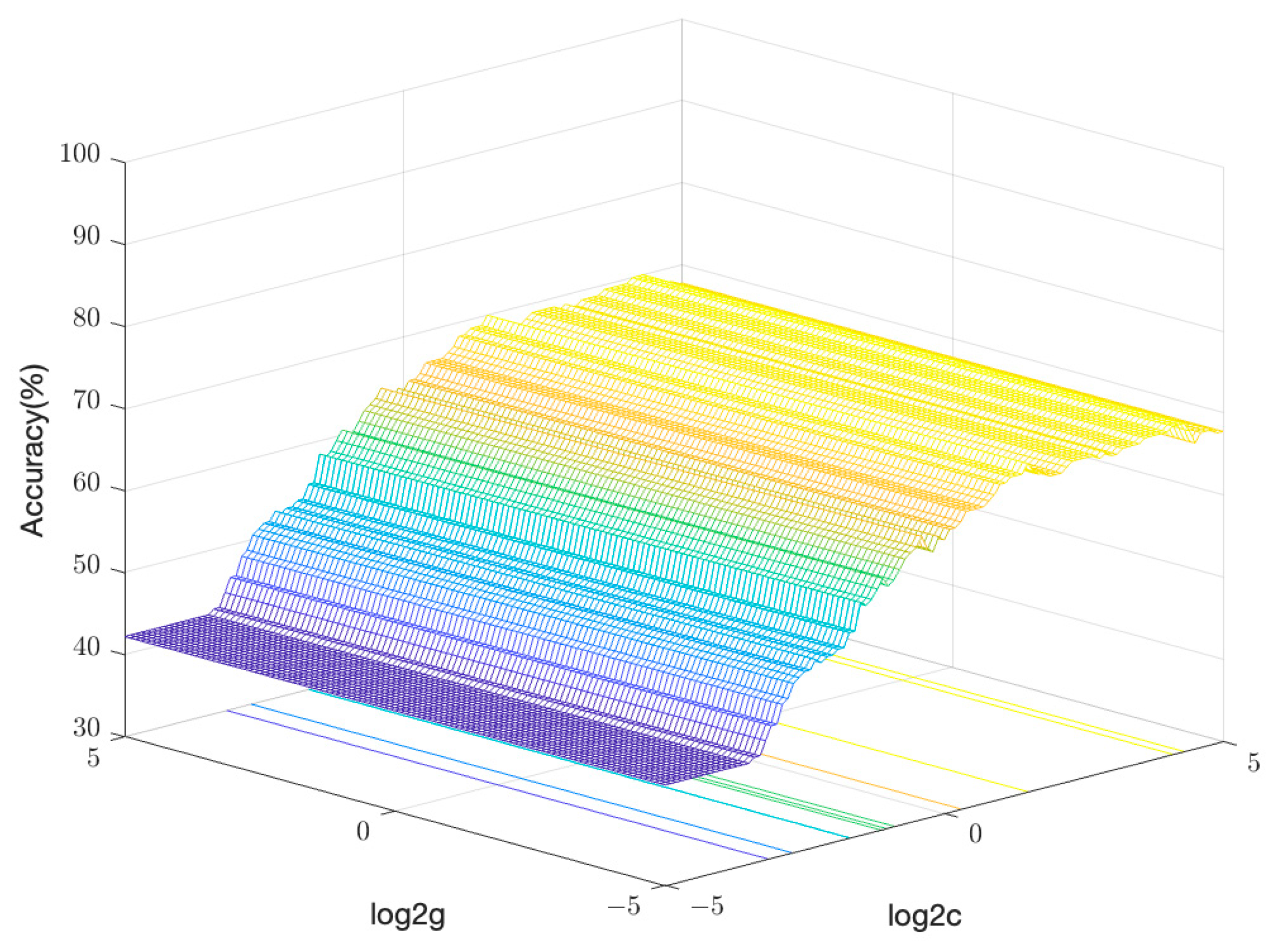
4.3. Accuracy Analysis

Eleven variables were selected as input variables for the model to determine the ideal number of tree species-sensitive features. The SVM was chosen to filter the number of features that strongly influenced the tree species category. Only the ranking of features obtained after thorough comparison was used in the final confirmation of the optimal number of features, and as the number of selected features steadily rose, each evaluation index was computed in sequence. The relationship between the number of features and the classification evaluation metric was examined using the SVM classifier. The entire dataset was split into two parts, where 70% of the data was used as the training set and the remaining as the test set. Evaluation metrics, including accuracy, precision, recall, and F1-score, were used to evaluate the model, and the results are presented in Figure 3.
In Figure 3, it can be observed that an increase in the number of features led to a rise in the overall accuracy of all evaluation indices. When six features were present, the F1-score reached its maximum value of 0.662. However, beyond a feature index of eight, the accuracy was found to be inversely associated with the number of features, and the total accuracy, precision, and recall all reached their optimal values at this point.
To optimize the hyperparameters of SVM, grid search methods were employed, where the penalty function and kernel function’s parameter ranges were varied between 2−5 and 25 at a step size of 0.1. The K-fold cross-validation method was used for the model validation, splitting the dataset into five groups as k was set to five in this experiment. During each of the five algorithm iterations, the model was trained on four datasets, while one of these five sets was used as a test set to check the accuracy of the model’s classification. Finally, the overall performance of the model was assessed using the average of evaluation metrics calculated from the test set. Figure 4 illustrates the optimization process of the grid search algorithm for parameters in the image statistical feature subset of different tree species. Upon exploring all possible combinations of hyperparameters, the best classification accuracy achieved on the dataset was 0.7, with an ideal parameter set of (2.83, 0.031).

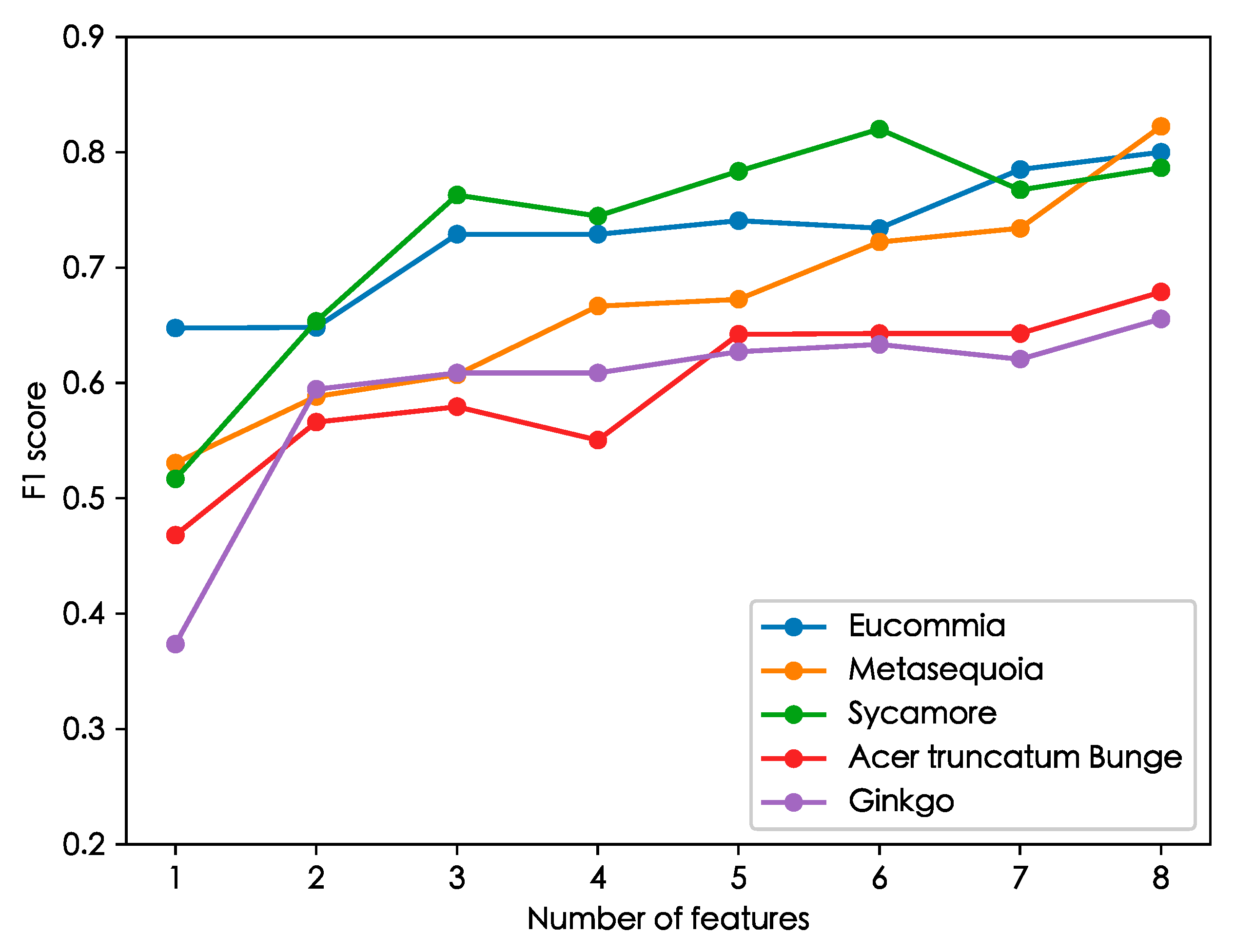
4.4. The Sensitivity Features Analysis

Table 3 displays the average of the two feature order indicators for each dimension feature. Moreover, the table highlights the significant differences in feature sensitivity across various tree species categories. However, Weibull_distribution.1 consistently ranked high across all tree species categories.
When calculating the ensitivity features of a specific category of five types of tree species images, 80 samples from that category were chosen as the training set. The test set was created by combining the remaining 20 samples with 20 samples from each category of tree species that were chosen at random. The number of features gradually increased in the order from front to back as the input of the model of Deep SVDD for training.
The F1-score was utilized to determine the optimal number of sensitive features for each tree species category. The subset of sensitive features required for the category was obtained when the F1-score reached its overall optimal value or attained a value of 0.7.
Figure 5 illustrates that as the number of features increased, the accuracy of the final indexes for Eucommia and Metasequoia reached 0.8. For the Sycamore, the F1-score peaked at 0.82 when the number of features reached six. The evaluation indicators for the two species of Acer truncatum Bunge and Ginkgo ingot displayed an initial increase, followed by a decline, and then increased again, with the overall evaluation index tending to increase as the number of features increased. At the maximum number of features, the F1-score of these two tree species reached the maximum values of 0.679 and 0.655, respectively.
Hence, as the number of features increased, it became possible to obtain the subset of sensitive features for various tree species categories. The testing of five categories of tree species, including Eucommia, Metasequoia, Sycamore, Acer truncatum Bunge, and Ginkgo, resulted in obtaining 3, 6, 6, 8, and 8 sensitive feature sets, respectively, thereby determining the set of sensitive features for each tree species.
Among these sets of sensitive features, the optimal feature combination for characterizing Eucommia comprised Weibull_distribution.1, Wavelet coefficients.25, and Wavelet_coefficients.72. Meanwhile, Weibull_distribution.1, Texture_property.4, Wavelet coefficients.47, Wavelet coefficients.25, Wavelet_coefficients.72, and Shape_property.1 were the best feature combinations for Metasequoia. In the case of Sycamore, the most effective feature subset consisted of Wavelet coefficients.47, Shape_property.1, Weibull_distribution.1, mean_s, Wavelet coefficients.25, and Texture_property.4. Finally, the feature subsets that best described Acer truncatum Bunge and Ginkgo were characterized by Shape_property.1, Texture_property.4, mean_s, Weibull_distribution.1, Wavelet_coefficients.11, Wavelet_coefficients.25, Wavelet_coefficients.47, and Wavelet_coefficients.72. However, the two types of tree species exhibited varying degrees of sensitivity to different features.

4.5. Validation

To validate the sensitive feature subsets of different tree species, the accuracy of the results was analyzed and verified. We only selected the corresponding feature value and regarded the category of this tree species as a positive sample, with other samples considered negative to verify the validity of a particular tree species’ sensitive feature subset. Five iterations of the algorithm were performed to ensure accuracy. The results, along with the various evaluation indicators, are presented in Table 4. It should be noted that the classification precision for Sycamore was 0.771, and all five tree species obtained F1-score exceeding 0.7. This demonstrates that the sensitive feature subsets of different tree species can effectively capture their unique features.

5. Conclusions

At present, image statistical properties are widely used and are powerful descriptive features in image processing [33]. The image statistical properties of tree species are essentially digital and quantitative descriptions of tree species characteristics, which are highly objective and comparable [34]. The extraction and analysis of these features can provide important data support and reference for tree species classification, ecological research, growth environment analysis, and ecological protection [35].
However, it is important to note that not all image statistical properties are equally correlated with the tree species. For example, certain features may be more relevant to problems such as pest detection or disease identification [36]. Problems such as tree species identification and classification can be realized by using features that are highly correlated with the tree species [37]. Furthermore, the accuracy of the 3D reconstructions of forest scenes can also be improved by using features that are less linked to tree species [38]. To identify the most relevant features for tree species variables and understand the sensitive feature subsets among diverse tree species, we employed various image statistical properties to quantify the tree images. Additionally, we analyzed the correlation between the image statistical properties and tree species categories. Eventually, we identified a subset of sensitive features for each tree species and verified the feasibility of our method. These experimental results emphasize the importance of carefully selecting image features for specific forestry tasks and demonstrate the potential of image-based methods for tree species analysis.
The SVM is a widely utilized classification algorithm in the field of forestry [39]. The performance of the SVM model in representing the tree species was assessed by calculating various evaluation metrics. It should be noted that not all features have a high correlation with the tree species variable, meaning that having more features does not necessarily lead to higher classification accuracy for tree species [40]. Feature selection is an essential part of feature engineering, which aims to choose the most relevant features from all the features [41]. The filter method is commonly used to identify the most significant feature subset that is highly correlated with the target label. This method is favored for its simplicity and broad applicability across diverse domains [42]. When classifying tree species using a limited number of features, enhancing the additional features can significantly increase the distinction between different tree species. Nevertheless, beyond a certain threshold of the number of features, adding more features does not significantly improve tree species classification and recognition [43]. Once the saturation point of the number of features has been reached, adding more features will lead to data redundancy, which can negatively affect the model performance and reduce its effectiveness. The results demonstrate that the correlation of image statistical properties with tree species variables does not always increase with the number of features. By combining the filtering method with SVM, we identified eight feature subsets that have the strongest correlation with the tree species categories.
Furthermore, feature importance measures are commonly employed for analyzing feature ranking problems and assessing the global sensitivity of classification models for each feature independently [44]. At the same time, feature evaluation and selection techniques based on SVDD can also be applied to feature selection in one-class classification problems [45]. However, the use of SVDD to analyze tree species sensitivity feature subsets is a novel research topic.
In this study, we observed differences in the sensitivity feature subsets among various tree species. The F1-score of all tree species was higher than 0.7 when using the sensitive feature subset of each tree species to verify its effectiveness. The experimental results demonstrate that our proposed method is effective in identifying sensitive feature subsets in tree species classification. This method can provide valuable insights into the development of more efficient methods for identifying tree species, ultimately contributing to the management and conservation of forest ecosystems. Nonetheless, our dataset was limited to certain tree species and geographic locations. While providing valuable insights and results, further research is required to explore the model’s performance on datasets from other regions with different tree species and variations in image acquisition conditions. Understanding the relationship between image statistical properties and other tree species can facilitate the model’s applicability to broader scenarios and enhance the evaluation metrics of algorithmic classification. Future studies could focus on expanding the dataset to include a more comprehensive range of tree species and geographic locations to enhance the model’s robustness. Additionally, exploring other factors that can affect the model’s performance, such as environmental conditions and image quality, could open up new avenues of research to further optimize the model for practical applications under real-world conditions.

Author Contributions

Conceptualization, X.S. and J.K.; methodology, X.S.; software, X.S.; validation, X.S. and J.K.; formal analysis, X.S.; investigation, X.S.; resources, X.S. and J.K.; data curation, X.S.; writing—original draft, X.S.; visualization, X.S.; supervision, J.K.; project administration, J.K. All authors have read and agreed to the published version of the manuscript.

Funding

This research was funded by the National Natural Science Foundation of China (No. 32071680).

Data Availability Statement

Test methods and data are available from the authors upon request.

Conflicts of Interest

The authors declare no conflict of interest.

References

  1. Dugesar, V.; Satish, K.V.; Pandey, M.K.; Srivastava, P.K.; Petropoulos, G.P.; Anand, A.; Behera, M.D. Impact of Environmental Gradients on Phenometrics of Major Forest Types of Kumaon Region of the Western Himalaya. Forests 2022, 13, 1973. [Google Scholar] [CrossRef]
  2. Garforth, J.; Webb, B. Visual Appearance Analysis of Forest Scenes for Monocular SLAM. In Proceedings of the 2019 International Conference on Robotics and Automation (ICRA), Montreal, QC, Canada, 20–24 May 2019; IEEE: Piscataway, NJ, USA, 2019; pp. 1794–1800. [Google Scholar]
  3. Liu, L.; Liu, Y.; Lv, Y.; Xing, J. LANet: Stereo Matching Network Based on Linear-Attention Mechanism for Depth Estimation Optimization in 3D Reconstruction of Inter-Forest Scene. Front. Plant Sci. 2022, 13, 978564. [Google Scholar] [CrossRef]
  4. Xu, R.; Lin, H.; Lu, K.; Cao, L.; Liu, Y. A Forest Fire Detection System Based on Ensemble Learning. Forests 2021, 12, 217. [Google Scholar] [CrossRef]
  5. Lebedev, V.G.; Lebedeva, T.N.; Chernodubov, A.I.; Shestibratov, K.A. Genomic Selection for Forest Tree Improvement: Methods, Achievements and Perspectives. Forests 2020, 11, 1190. [Google Scholar] [CrossRef]
  6. Qin, H.; Zhou, W.; Yao, Y.; Wang, W. Individual Tree Segmentation and Tree Species Classification in Subtropical Broadleaf Forests Using UAV-Based LiDAR, Hyperspectral, and Ultrahigh-Resolution RGB Data. Remote Sens. Environ. 2022, 280, 113143. [Google Scholar] [CrossRef]
  7. Cerutti, G.; Tougne, L.; Mille, J.; Vacavant, A.; Coquin, D. Understanding Leaves in Natural Images–a Model-Based Approach for Tree Species Identification. Comput. Vis. Image Underst. 2013, 117, 1482–1501. [Google Scholar] [CrossRef]
  8. Fiel, S.; Sablatnig, R. Automated Identification of Tree Species from Images of the Bark, Leaves or Needles. In Proceedings of the Computer Vision Winter Workshop, Mitterberg, Austria, 2–4 February 2010. [Google Scholar]
  9. Bambil, D.; Pistori, H.; Bao, F.; Weber, V.; Alves, F.M.; Gonçalves, E.G.; de Alencar Figueiredo, L.F.; Abreu, U.G.; Arruda, R.; Bortolotto, I.M. Plant Species Identification Using Color Learning Resources, Shape, Texture, through Machine Learning and Artificial Neural Networks. Environ. Syst. Decis. 2020, 40, 480–484. [Google Scholar] [CrossRef]
  10. Fekri-Ershad, S. Bark Texture Classification Using Improved Local Ternary Patterns and Multilayer Neural Network. Expert Syst. Appl. 2020, 158, 113509. [Google Scholar] [CrossRef]
  11. Wang, T.; Zhang, H.; Lin, H.; Fang, C. Textural—Spectral Feature-Based Species Classification of Mangroves in Mai Po Nature Reserve from Worldview-3 Imagery. Remote Sens. 2015, 8, 24. [Google Scholar] [CrossRef]
  12. Chen, X.; Wang, B.; Gao, Y. Symmetric Binary Tree Based Co-Occurrence Texture Pattern Mining for Fine-Grained Plant Leaf Image Retrieval. Pattern Recognit. 2022, 129, 108769. [Google Scholar] [CrossRef]
  13. Cetin, Z.; Yastikli, N. The Use of Machine Learning Algorithms in Urban Tree Species Classification. IJGI 2022, 11, 226. [Google Scholar] [CrossRef]
  14. Park, G.; Lee, Y.-G.; Yoon, Y.-S.; Ahn, J.-Y.; Lee, J.-W.; Jang, Y.-P. Machine Learning-Based Species Classification Methods Using DART-TOF-MS Data for Five Coniferous Wood Species. Forests 2022, 13, 1688. [Google Scholar] [CrossRef]
  15. Pantazi, X.E.; Moshou, D.; Tamouridou, A.A. Automated Leaf Disease Detection in Different Crop Species through Image Features Analysis and One Class Classifiers. Comput. Electron. Agric. 2019, 156, 96–104. [Google Scholar] [CrossRef]
  16. Zhao, H.; Zhong, Y.; Wang, X.; Hu, X.; Luo, C.; Boitt, M.; Piiroinen, R.; Zhang, L.; Heiskanen, J.; Pellikka, P. Mapping the Distribution of Invasive Tree Species Using Deep One-Class Classification in the Tropical Montane Landscape of Kenya. ISPRS J. Photogramm. Remote Sens. 2022, 187, 328–344. [Google Scholar] [CrossRef]
  17. Pan, H.; Xu, H.; Zheng, J.; Su, J.; Tong, J. Multi-Class Fuzzy Support Matrix Machine for Classification in Roller Bearing Fault Diagnosis. Adv. Eng. Inform. 2022, 51, 101445. [Google Scholar] [CrossRef]
  18. Ibrahim, I.; Khairuddin, A.S.M.; Abu Talip, M.S.; Arof, H.; Yusof, R. Tree Species Recognition System Based on Macroscopic Image Analysis. Wood Sci. Technol. 2017, 51, 431–444. [Google Scholar] [CrossRef]
  19. Wheeler, E.A. Inside Wood–A Web Resource for Hardwood Anatomy. Iawa J. 2011, 32, 199–211. [Google Scholar] [CrossRef]
  20. Zhang, Z.; Deng, X. Anomaly Detection Using Improved Deep SVDD Model with Data Structure Preservation. Pattern Recognit. Lett. 2021, 148, 1–6. [Google Scholar] [CrossRef]
  21. Sun, Y.; Huang, J.; Ao, Z.; Lao, D.; Xin, Q. Deep Learning Approaches for the Mapping of Tree Species Diversity in a Tropical Wetland Using Airborne LiDAR and High-Spatial-Resolution Remote Sensing Images. Forests 2019, 10, 1047. [Google Scholar] [CrossRef]
  22. Haralick, R.M. Statistical and Structural Approaches to Texture. Proc. IEEE 1979, 67, 786–804. [Google Scholar] [CrossRef]
  23. Michałowska, M.; Rapiński, J. A Review of Tree Species Classification Based on Airborne LiDAR Data and Applied Classifiers. Remote Sens. 2021, 13, 353. [Google Scholar] [CrossRef]
  24. Torralba, A.; Oliva, A. Statistics of Natural Image Categories. Netw. Comput. Neural Syst. 2003, 14, 391. [Google Scholar] [CrossRef]
  25. Yanulevskaya, V.; Geusebroek, J.-M. Significance of the Weibull Distribution and Its Sub-Models in Natural Image Statistics. In Proceedings of the VISAPP 2009—Proceedings of the Fourth International Conference on Computer Vision Theory and Applications, Lisbon, Portugal, 5–8 February 2009; pp. 355–362. [Google Scholar]
  26. Mittal, A.; Moorthy, A.K.; Bovik, A.C. No-Reference Image Quality Assessment in the Spatial Domain. IEEE Trans. Image Process. 2012, 21, 4695–4708. [Google Scholar] [CrossRef]
  27. Sawant, S.S.; Manoharan, P. Unsupervised Band Selection Based on Weighted Information Entropy and 3D Discrete Cosine Transform for Hyperspectral Image Classification. Int. J. Remote Sens. 2020, 41, 3948–3969. [Google Scholar] [CrossRef]
  28. You, N.; Han, L.; Zhu, D.; Song, W. Research on Image Denoising in Edge Detection Based on Wavelet Transform. Appl. Sci. 2023, 13, 1837. [Google Scholar] [CrossRef]
  29. Jo, I.; Lee, S.; Oh, S. Improved Measures of Redundancy and Relevance for MRMR Feature Selection. Computers 2019, 8, 42. [Google Scholar] [CrossRef]
  30. Urbanowicz, R.J.; Meeker, M.; La Cava, W.; Olson, R.S.; Moore, J.H. Relief-Based Feature Selection: Introduction and Review. J. Biomed. Inform. 2018, 85, 189–203. [Google Scholar] [CrossRef]
  31. Kononenko, I.; Šimec, E.; Robnik-Šikonja, M. Overcoming the Myopia of Inductive Learning Algorithms with RELIEFF. Appl. Intell. 1997, 7, 39–55. [Google Scholar] [CrossRef]
  32. Lorena, L.H.; Carvalho, A.C.; Lorena, A.C. Filter Feature Selection for One-Class Classification. J. Intell. Robot. Syst. 2015, 80, 227–243. [Google Scholar] [CrossRef]
  33. Simoncelli, E.P.; Olshausen, B.A. Natural Image Statistics and Neural Representation. Annu. Rev. Neurosci. 2001, 24, 1193–1216. [Google Scholar] [CrossRef]
  34. Ratajczak, R.; Bertrand, S.; Crispim-Junior, C.F.; Tougne, L. Efficient Bark Recognition in the Wild. In Proceedings of the International Conference on Computer Vision Theory and Applications (VISAPP 2019), Prague, Czech Republic, 25–27 February 2019. [Google Scholar]
  35. Yadav, A.R.; Anand, R.S.; Dewal, M.L.; Gupta, S. Performance Analysis of Discrete Wavelet Transform Based First-Order Statistical Texture Features for Hardwood Species Classification. Procedia Comput. Sci. 2015, 57, 214–221. [Google Scholar] [CrossRef]
  36. Arivazhagan, S.; Shebiah, R.N.; Ananthi, S.; Varthini, S.V. Detection of Unhealthy Region of Plant Leaves and Classification of Plant Leaf Diseases Using Texture Features. Agric. Eng. Int. CIGR J. 2013, 15, 211–217. [Google Scholar]
  37. Barmpoutis, P.; Dimitropoulos, K.; Barboutis, I.; Grammalidis, N.; Lefakis, P. Wood Species Recognition through Multidimensional Texture Analysis. Comput. Electron. Agric. 2018, 144, 241–248. [Google Scholar] [CrossRef]
  38. Garforth, J.; Webb, B. Lost in the Woods? Place Recognition for Navigation in Difficult Forest Environments. Front. Robot. AI 2020, 7, 541770. [Google Scholar] [CrossRef] [PubMed]
  39. Pang, Z.; Zhang, G.; Tan, S.; Yang, Z.; Wu, X. Improving the Accuracy of Estimating Forest Carbon Density Using the Tree Species Classification Method. Forests 2022, 13, 2004. [Google Scholar] [CrossRef]
  40. Sothe, C.; Dalponte, M.; de Almeida, C.M.; Schimalski, M.B.; Lima, C.L.; Liesenberg, V.; Miyoshi, G.T.; Tommaselli, A.M.G. Tree Species Classification in a Highly Diverse Subtropical Forest Integrating UAV-Based Photogrammetric Point Cloud and Hyperspectral Data. Remote Sens. 2019, 11, 1338. [Google Scholar] [CrossRef]
  41. Li, J.; Cheng, K.; Wang, S.; Morstatter, F.; Trevino, R.P.; Tang, J.; Liu, H. Feature Selection: A Data Perspective. ACM Comput. Surv. 2018, 50, 1–45. [Google Scholar] [CrossRef]
  42. Chandrashekar, G.; Sahin, F. A Survey on Feature Selection Methods. Comput. Electr. Eng. 2014, 40, 16–28. [Google Scholar] [CrossRef]
  43. Fu, B.; Liu, M.; He, H.; Lan, F.; He, X.; Liu, L.; Huang, L.; Fan, D.; Zhao, M.; Jia, Z. Comparison of Optimized Object-Based RF-DT Algorithm and SegNet Algorithm for Classifying Karst Wetland Vegetation Communities Using Ultra-High Spatial Resolution UAV Data. Int. J. Appl. Earth Obs. Geoinf. 2021, 104, 102553. [Google Scholar] [CrossRef]
  44. Razmjoo, A.; Xanthopoulos, P.; Zheng, Q.P. Online Feature Importance Ranking Based on Sensitivity Analysis. Expert Syst. Appl. 2017, 85, 397–406. [Google Scholar] [CrossRef]
  45. Jeong, Y.-S.; Kang, I.-H.; Jeong, M.-K.; Kong, D. A New Feature Selection Method for One-Class Classification Problems. IEEE Trans. Syst. Man Cybern. Part C 2012, 42, 1500–1509. [Google Scholar] [CrossRef]
Figure 1. Typical picture in the tree species dataset.
Forests 14 01057 g001
Figure 2. Violin plots of the tree species.
Forests 14 01057 g002aForests 14 01057 g002b
Figure 3. Comparison of accuracy of selected feature subsets using SVM classifier by combining multiple feature selection ranking methods.
Forests 14 01057 g003
Figure 4. Optimization diagram of the grid search algorithm parameters.
Forests 14 01057 g004
Figure 5. Relationship between the number of features and F1-score.
Forests 14 01057 g005
Table 1. A summary of the image's statistical properties.
The Feature NameDimension
mean_h, mean_s, mean_v,3
Texture property5
Shape property7
Power spectrum8
Weibull coefficients2
MSCN coefficients18
DCT coefficients4
Wavelet coefficients88
Table 2. Results of applying average feature rank to the tree species dataset.
FeatureSpearmanmRMRRelieFCombined Ranking
Shape_property.18826
Texture_property.49112
mean_s3442
Weibull_distribution.11631
MSCN coefficients.115101010
Wavelet_coefficients.117354
Wavelet_coefficients.236999
Wavelet_coefficients.251764
Wavelet_coefficients.291110611
Wavelet_coefficients.4745106
Wavelet_coefficients.7210288
Table 3. Results of applying average feature rank to the tree species dataset.
EucommiaMetasequoia Sycamore Acer truncatum Bunge Ginkgo
Shape_property.166251
Texture_property.452672
mean_s68426
Weibull_distribution.111323
Wavelet_coefficients.1147768
Wavelet coefficients.2524514
Wavelet_coefficients.4782145
Wavelet_coefficients.7234886
Table 4. Multiple evaluation metrics for tree species.
PrecisionRecallF1-score
Eucommia0.7310.6610.695
Sycamore0.7710.6940.736
Ginkgo0.6740.5820.639
Metasequoia0.7160.5950.647
Acer truncatum Bunge0.6490.6120.626
Disclaimer/Publisher’s Note: The statements, opinions and data contained in all publications are solely those of the individual author(s) and contributor(s) and not of MDPI and/or the editor(s). MDPI and/or the editor(s) disclaim responsibility for any injury to people or property resulting from any ideas, methods, instructions or products referred to in the content.

