MISF: A Method for Measurement of Standing Tree Size via Multi-Vision Image Segmentation and Coordinate Fusion

Abstract

With the development of computer vision technology, its applications in forestry are steadily becoming wider. To address the problems of inconvenience in transporting unmanned aerial vehicles (UAVs), as well as the complex operation of large instruments for measurement, a new method based on multi-vision image segmentation and coordinate fusion (MISF) is proposed in this paper for measuring the size of standing trees. In MISF, after images of a standing tree are captured using a camera from multiple angles, a semantic segmentation method based on deep learning is used to segment the main body of the standing tree and automatically detect the edge feature points. Next, the effects of visual field splicing and fusion are analyzed collaboratively using the correlations among images, so as to restore the three-dimensional spatial information of the feature points of the tree to be measured. Lastly, the size attributes of the standing tree, such as height, diameter at breast height (DBH), and crown width, are automatically measured. The urban environment measurement experiment showed that the relative errors of tree height, DBH, and crown width measured using the proposed method, i.e., MISF, were 1.89%, 2.42%, and 3.15%, respectively, representing a significant enhancement compared with binocular measurement. On the one hand, the experimental results exhibited a high degree of measurement accuracy; therefore, MISF can be used for the management inventory of typical forests. On the other hand, MISF cannot be used if a tree’s images cannot be acquired due to environmental or other reasons.

1. Introduction

In forestry, collecting tree-related information is essential for analyzing forestry resources [1,2]. This information consists of the height, diameter at breast height (DBH), and other data of standing trees. Traditional methods measure standing trees using rulers or other measuring tools [3], which is time-consuming and labor-intensive. On the other hand, precise equipment, such as electronic theodolites and total stations, is inconvenient to use because of its relatively complex operation [4,5].

At present, most measurements of standing trees are conducted using hardware, such as laser unmanned aerial vehicles (UAVs), terrestrial laser scanners, and other height-equipment measurement methods [6,7]. For example, Li et al. [8] proposed a new tree diameter measurement instrument developed using a self-reset displacement sensor, which was equipped with a personal computer to enable the measurement, transmission, storage, and analysis of tree diameters. Olofsson et al. [9] proposed a method to automatically detect trees in a TLS-scanned field plot, classify the laser return as either into stem or canopy for each of the detected trees, and extract forest variables from the classified data. Yuan et al. [10] developed a measuring device for tree DBH and tree height using a high-precision laser ranging sensor. The combination of the accurate identification and segmentation of standing trees using multi-vision measurement is less well-studied. The traditional fixed binocular measurement model still has certain limitations and flexibility, whereas multi-vision measurement can make up for these shortcomings, improving the stability and accuracy [11,12].

With the continuous development of science and technology mirroring the progress of computer vision, more and more measurement methods have been proposed. Adilson et al. [13] presented an automatic technique for the mapping and measurement of individual tree stems using vertical terrestrial images collected with a fisheye camera. Krause et al. [14] used UAV photogrammetry to semiautomatically obtain the height of standing trees. Ramli et al. [15] proposed the use of an UAV to capture images of oil palm trees, followed by the generation of digital models and the processing of orthophoto images using Agisoft software; then, they calculated the crown size of oil palm trees by implementing the seed generation tool of the quantum geographic information system (QGIS) and the system for automatic geological analysis (SAGA) segmentation methods. Wu et al. [16] proposed a method based on monocular vision to measure the DBH of standing trees by photographing a single image using a camera.

Addressing the shortcomings identified from the literature review, a flexible method for the measurement of standing trees using multi-vision image segmentation and coordinate fusion (MISF) is proposed in this paper.

The main contributions of this paper include three aspects:

(1) A new multi-view measurement model (MISF) for standing trees is proposed, combining the advantages of image processing to realize the noncontact automatic measurement of standing trees. A camera is used to capture standing trees from three angles, thereby obtaining a wider field of view and improving the accuracy of the matching position of feature points.

(2) The image matching algorithm SURF (speeded up robust features) is improved to enable the matching of feature points in standing tree images. The original SURF algorithm has good stability and low computing complexity. However, the SURF algorithm transforms color images into grayscale, thus partially losing the color information. In view of this problem, we improved the algorithm SURF by adding a 48-dimensional RGB color information descriptor. Accordingly, the color information could be well-retained compared with the original SURF algorithm, thus increasing the matching performance and the robustness of the algorithm.

(3) Extensive experiments were conducted so as to evaluate the performance of the proposed method (MISF). In the experiments, some tree size attributes such as height, DBH, and crown width were measured using MISF to verify its applicability. Its performance was also compared with traditional binocular measurement and other measurement methods in the literature. The experiments revealed that the performance of MISF could meet the requirements of forest management inventory.

The method proposed in this paper achieves a significant improvement in measurement accuracy over the traditional binocular measurement method, improving the practical application. The measurement errors of tree height, diameter at breast height, and crown width were comparable with those of other measurement methods, in addition to meeting the accuracy requirements for the continuous inventory of forest resources.

2. Materials and Methods

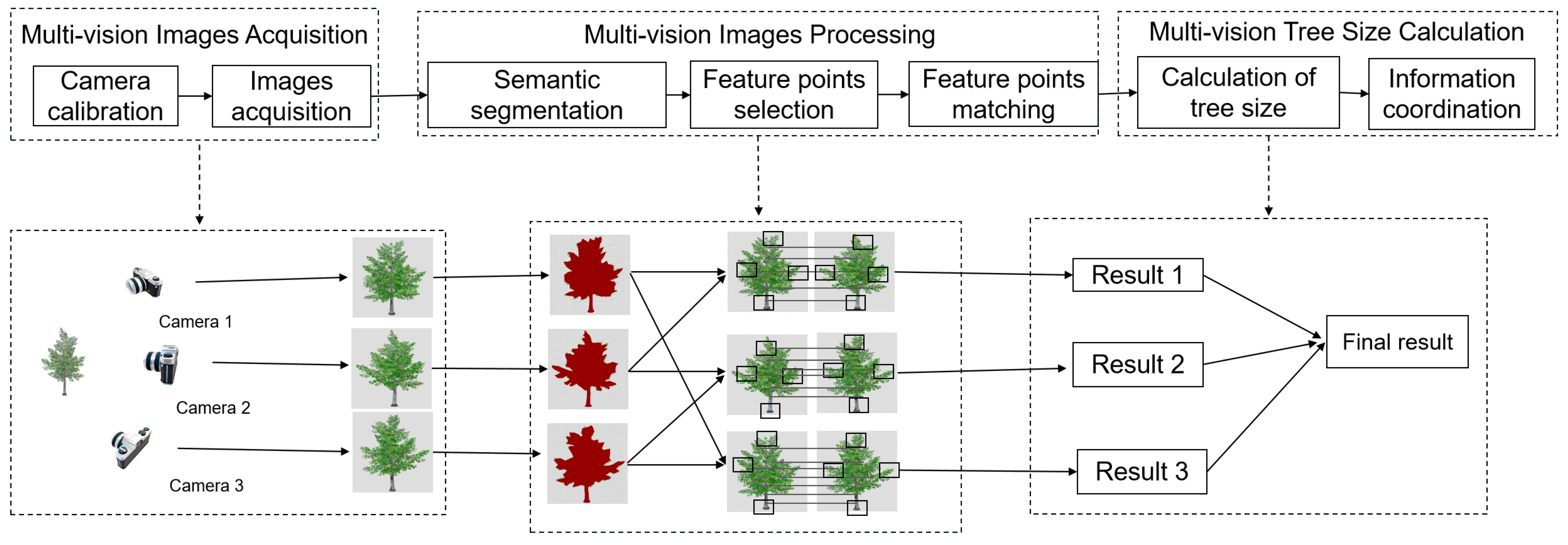
2.1. Main Ideas

In the theory of close-up photogrammetry, the utilization of a single camera to capture an image in order to acquire stereo information regarding the target is referred to as monocular measurement. This method is low cost but limited to obtaining only two-dimensional information about the target, and cannot ascertain the distance of the measured target. On the other hand, binocular measurement involves using two cameras to capture images from different perspectives, thereby enabling the acquisition of three-dimensional coordinate information of the target. However, this method is constrained by a certain range of field of view and requires the use of two parallel cameras, which may introduce some degree of error due to human factors.

On this basis, the present paper proposes an innovation that incorporates the intersection measurement method [17]. This approach eliminates the need for parallel optical axes between cameras and instead involves capturing multiple images from varying angles of a standing tree to reconstruct its three-dimensional information. During the image capture process, it is only necessary to ensure that the main body of the tree being measured is within the common field of view among the three shooting perspectives. This condition ensures that the common field of view is sufficiently large to enhance measurement accuracy without requiring strict location specifications.

The main concept behind the proposed method for measuring the size of standing trees, known as MISF, is based on multi-vision image segmentation and coordinate fusion, as illustrated in Figure 1. To facilitate measurement, three binocular subsystems were established using cameras to capture images of standing trees from varying perspectives. In the following step of the method, the segmentation of standing trees in the images is performed to accurately identify their positions. Next, three sets of binocular sub-models are utilized to obtain the group of largest measurements via comparison. The final standing-tree factor measurement is achieved through the fusion of the results obtained from the segmentation of standing trees and size measurement.

When compared to binocular stereo vision measurement methods and height equipment measurement techniques, such as UAV and scanner 3D reconstruction, the MISF method exhibits distinct differences and notable advantages in several key areas, including:

(1) The MISF method employs a deep learning-based image segmentation technique to extract the standing tree factor, which enables automatic contour extraction and segmentation results without requiring manual intervention. As a result, the MISF method is characterized by enhanced efficiency and automation, significantly reducing manpower and time costs.

(2) Compared to a conventional binocular camera, the MISF method can acquire additional views and feature point information. While binocular cameras only capture two parallel-view images, resulting in improved accuracy, the MISF method employs three cameras that can cross-verify each other, thereby increasing the reliability of measurement results.

(3) When compared to high equipment measurement methods, the MISF method is characterized by a lower cost. This approach eliminates the need for repeated measurements by humans in the field; instead, the camera position only needs to be fixed once to achieve repeatable measurements.

2.2. Multiple Vision Image Acquisition

2.2.1. Single Camera Calibration

The MISF method adopts Zhang’s [18,19] camera calibration approach using a checkerboard for calibration. This method accounts for both radial and tangential distortion and facilitates the capture of multiple sets of images from various angles and directions by moving the calibration board. This flexible, convenient, and accurate technique requires a checkerboard image containing 9 x 12 angle points, with each checkerboard measuring 15mm in physical length, as shown in Figure 2.

The calibration process for a single camera primarily comprises four steps. First, the physical coordinates of the feature points on the calibration board are optimized to solve the homologous matrix. Second, the stack matrix B is calculated during the calibration process, which allows for the acquisition of the camera’s intrinsic parameter matrix. Third, the extrinsic parameters of the camera are solved, followed by the derivation of the camera distortion coefficients.. Fourth, the maximum likelihood method is utilized to optimize the intrinsic parameters and improve the estimation accuracy. Each step is described in detail below.

(1) Solving homologous matrix

After the physical coordinates of the characteristic points on the calibration plate were transposed, the homologous matrix was solved. As for computer vision, a homologous matrix is defined as a two-dimensional coordinate point mapped onto a camera image. Assuming that the coordinate of the feature point is $Q={\left[\begin{array}{ccc}{X}_m& Y_m& Z_m\end{array}\right]}^T$, the coordinates of the image on the camera are $q={\left[\begin{array}{ccc}u& v& 1\end{array}\right]}^T$. The monograph relationship between the calibration plate plane and the camera image plane is shown as Equation (1):

$$sq=P\left[R,T\right]X$$

(1)

In Equation (1), s is the scale factor, P represents the parameter matrix of the camera, R represents the rotation matrix, and T denotes the translation vector. Suppose that $\left[R,T\right]=\left[\begin{array}{ccc}{r}_1& r_2& \begin{array}{cc}{r}_3& t\end{array}\end{array}\right]$, the world coordinate system is established on the checkerboard in the calibration process, namely, Z = 0 in the checkerboard plane, and then the homologous matrix D can be derived by $s\left[\begin{array}{c}u\\ v\\ 1\end{array}\right]=D\left[\begin{array}{c}X\\ Y\\ 1\end{array}\right]$.

(2) Calculation of camera internal parameter matrix

Through the above, the homologous matrix D follows the expression of Equation (2):

$$\mathrm{D}=\left[\begin{array}{ccc}{h}_1& h_2& h_3\end{array}\right]=\frac{P\left[\begin{array}{ccc}{r}_1& r_2& t\end{array}\right]}{s}$$

(2)

The camera intrinsic parameter matrix contains five unknowns, and the homologous matrix can generate two equations, so at least three calibration plates are required for calibration. For the convenience of later calculation, the stacking matrix B is assumed as Equation (3), where there are six unknowns. The vector b is assumed as Equation (4):

$$\mathrm{B}=P^{-T}{P}^{-1}=\left[\begin{array}{ccc}{B}_{11}& B_{12}& B_{13}\\ B_{21}& B_{22}& B_{23}\\ B_{31}& B_{32}& B_{33}\end{array}\right]$$

(3)

$$b={\left[\begin{array}{cccccc}{B}_{11}& B_{12}& B_{22}& B_{13}& B_{23}& B_{33}\end{array}\right]}^T$$

(4)

Then, the following Equation (5) is reached:

$$h_i^{T}B{h}_j=v_{ij}^{T}b$$

(5)

Because of the constraint of Equation (6) on the calibration process, it is necessary to obtain the matrix B through multiple checkerboard images, and finally to obtain the intrinsic parameter matrix P through Cholesky decomposition:

$$\left[\begin{array}{c}{v}_{12}^T\\ {\left(v_{11}-v_{22}\right)}^T\end{array}\right]b=0$$

(6)

(3) Solving the camera extrinsic parameters

According to Equation (2), let $\mathsf{\lambda }=\frac{1}{\mathrm{s}}$, then, Equation (7) can be derived:

$$\begin{array}{l}{r}_1=\lambda P^{-1}{h}_1\\ r_2=\lambda P^{-1}{h}_2\\ r_3=r_1\times r_2\\ t=\lambda P^{-1}{h}_3\end{array}$$

(7)

In Equation (7), $\mathsf{\lambda }=\frac{1}{\Vert {\mathrm{P}}^{-1}{\mathrm{h}}_1\Vert }=\frac{1}{\Vert {\mathrm{P}}^{-1}{\mathrm{h}}_2\Vert }$. Then, the extrinsic parameter matrix [R, T] of the camera can be calculated.

(4) Results optimization

According to the derivation of above equations, the results can be obtained under ideal conditions. However, in reality, the results are often affected by Gaussian noise, which usually leads to suboptimal results. Therefore, it is necessary to optimize the results. In MISF, the maximum likelihood estimation method is adopted to optimize the results, mainly optimizing the intrinsic parameters of the camera for single-camera calibration results.

Assuming that n calibration board images were acquired, each of which contains m corner points, the j-th corner point in the i-th image can be calculated using the above projection equations and the following Equation (8) can be obtained:

$$m\left(P,R_i,t_i,M_{ij}\right)=P\left[\left.R\right|t\right]M_{ij}$$

(8)

In Equation (8), P denotes the camera internal parameter matrix, R_i denotes the rotation matrix of the i-th image, and t_i denotes the translation vector of the i-th image. Thus, the corresponding likelihood function is established as Equation (9), and the Levenberg–Marquardt [20] algorithm is used to find the optimal solution.

$$\mathrm{L}\left(\mathrm{P},R_i,t_i,M_{ij}\right)=\frac{1}{\sqrt{2\pi }}e\frac{-{\displaystyle {\sum }_{i-1}^n{\displaystyle {\sum }_{j-1}^m{\left(\widehat{m}\left(\mathrm{P},R_i,t_i,M_{ij}\right)-m_{ij}\right)}^2}}}{{\sigma }^2}$$

(9)

The form of the distortion coefficient matrix is shown as Equation (10), where (u, v) is the ideal pixel coordinates, (u′, v′) represents the pixel coordinates that produce distortion in the real state, (u₀, v₀) represents the position of the main point on the image, (x, y) represents the continuous coordinates in the optimal state, and k₁, k₂ are the distortion coefficients of the first two terms.

$$\left[\begin{array}{cc}\left(u-u_0\right)\left(x^2+y^2\right)& \left(u-u_0\right){\left(x^2+y^2\right)}^2\\ \left(v-v_0\right)\left(x^2+y^2\right)& \left(v-v_0\right){\left(x^2+y^2\right)}^2\end{array}\right]\left[\begin{array}{c}{k}_1\\ k_2\end{array}\right]=\left[\begin{array}{c}{u}^{\prime }-u\\ v^{\prime }-v\end{array}\right]$$

(10)

Transform Equation (10) to the form Hk = d, which leads to Equation (11):

$$k={\left[k_1{k}_2\right]}^T={\left(H^{T}H\right)}^{-1}d$$

(11)

Finally, the distortion coefficient k is obtained, and the maximum likelihood estimation method is used to estimate the distortion coefficient accurately, as is shown in Equation (12).

$${{\displaystyle {\sum }_{i=1}^n{\displaystyle {\sum }_{j=1}^m‖\widehat{m}\left(P,k_1,k_2,R_i,t_i,M_{ij}\right)-m_{ij}‖}}}^2$$

(12)

2.2.2. Trinocular Vision Calibration

In MISF, the calibration method by Zhang [18,19] is adopted, which is used in the previous monocular camera calibration to obtain the intrinsic and extrinsic parameters of three cameras. However, in order to calculate the three-dimensional coordinates of feature points, it is also necessary to obtain the inter-camera visual parameters. Based on the results of individual camera calibration, coordinate transformation is used to achieve mutual calibration among the three cameras, as shown in Figure 3.

In the trinocular vision measurement model, the external parameters of camera 1, camera 2, and camera 3 are R_i and T_i (i = 1, 2, 3), respectively, and represent the relative position relationship between their respective cameras and their corresponding world coordinate system. For a point E to be measured, E_n represents its world coordinate position, E₁ represents the coordinates of camera 1 in the self-coordinate system, E₂ represents the coordinates of camera 2 in the self-coordinate system, and E₃ represents the coordinates of camera 3 in the self-coordinate system. They comply with Equation (13):

$$\begin{array}{l}{\mathrm{E}}_1=R_1{E}_n+T_1\\ {\mathrm{E}}_2=R_2{E}_n+T_2\\ {\mathrm{E}}_3=R_3{E}_n+T_3\end{array}$$

(13)

The rotation matrix and translation vector between camera 1 and camera 2 are R₁₂ and T₁₂, respectively, the rotation matrix and translation vector between camera 2 and camera 3 are R₂₃ and T₂₃, respectively, and the rotation matrix and translation vector between camera 3 and camera 1 are R₁₃ and T₁₃, respectively, so Equations (14)–(16) can be obtained:

$$\begin{array}{l}{\mathrm{R}}_{12}=R_2{R}_1^{-1}\\ T_{12}=T_2-R_2{R}_1^{-1}{T}_1\end{array}$$

(14)

$$\begin{array}{l}{\mathrm{R}}_{23}=R_3{R}_2^{-1}\\ T_{23}=T_3-R_3{R}_2^{-1}{T}_2\end{array}$$

(15)

$$\begin{array}{l}{\mathrm{R}}_{13}=R_3{R}_1^{-1}\\ T_{13}=T_3-R_3{R}_1^{-1}{T}_1\end{array}$$

(16)

After knowing the rotation matrix and translation vector of the three cameras, the position structure parameters of the trinocular vision measurement model can be calculated by Equations (14)–(16).

The calibration of the trinocular vision model is similar to the single camera calibration method. As the last step, the parameter values of three cameras (R₁₂, T₁₂), (R₂₃, T₂₃), and (R₁₃, T₁₃) are obtained using the Levenberg–Marquardt method for optimization. In the solution of the optimization, the internal parameters and distortion coefficients of the three cameras’ self-calibration will also change. That is to say, in the first measurement group, the original internal parameters of camera 1 and camera 2 are P₁ and P₂, and they are changed to ${\mathrm{P}}_{12}^1$ and ${\mathrm{P}}_{12}^2$ after optimization. Similarly, the internal parameters of the second and third measurement groups are optimized as ${\mathrm{P}}_{23}^2$, ${\mathrm{P}}_{23}^3$ and ${\mathrm{P}}_{13}^1$, ${\mathrm{P}}_{13}^3$, respectively. After nonlinear optimization, all parameters required for the calibration of the trinocular vision measurement model are obtained.

2.2.3. Image Acquisition

To ensure the inclusion of a common target standing-tree subject in all three images, we acquired images of the standing tree using a camera at three different locations. In contrast to the traditional binocular parallel measurement approach that requires keeping the optical axes parallel to each other, the MISF method proposed in this paper requires orienting the camera optical axes towards the target tree. To obtain images of standing trees from multiple directions, we recommend positioning the three cameras in a triangular configuration with a certain horizontal angle (30°–45°) between the optical axes of two adjacent cameras. The shooting schema is depicted in Figure 4.

2.3. Multiple Vision Image Processing

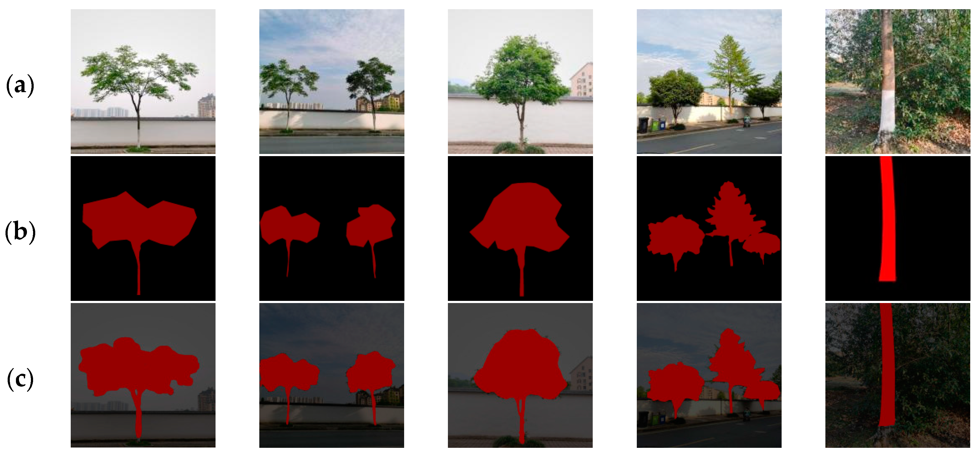
2.3.1. Semantic Segmentation of Tree Images Based on Deep Learning

In the real-world environment, photos often exhibit complex backgrounds with significant amounts of noise. To effectively extract the required size information of standing trees from images, image segmentation is crucial. Within MISF, we leverage SEMD, a lightweight model for standing-tree image segmentation that we previously proposed in [21]

The SEMD segmentation model utilizes MobileNetV2 + SENet as the backbone network in the encoder section. This structure can calculate and extract features with any resolution, and the ratio of the input image spatial resolution to the output image spatial resolution is used as the output stride. To perform multi-scale fusion, different dilated convolutions are employed to process features calculated by MobileNetV2 + SENet, which effectively reduces the running time without compromising segmentation accuracy. In the decoder section, a similar convolutional network is utilized to reduce the number of information channels and address difficulties encountered during training due to an excess of low-feature channels.

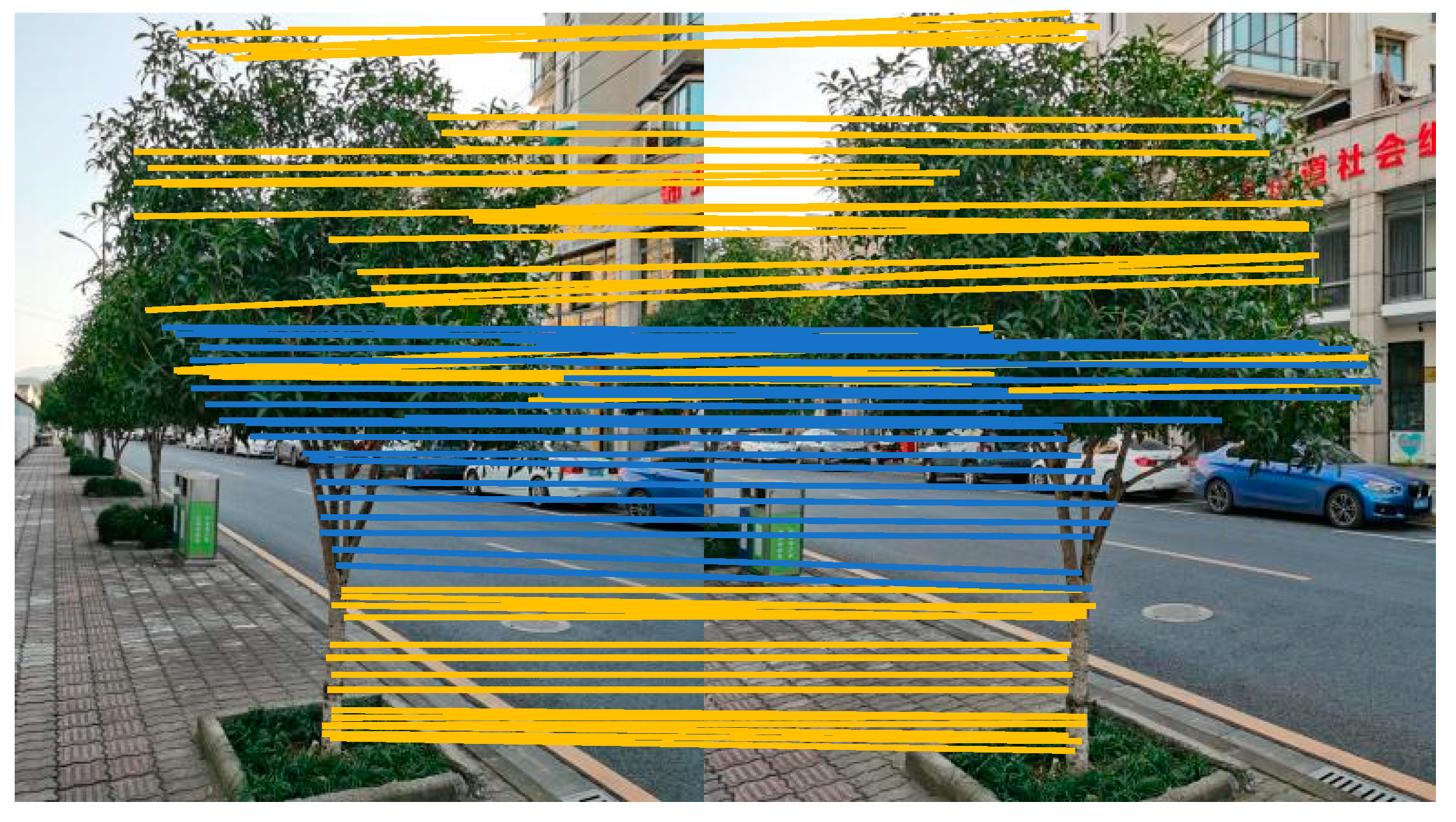
2.3.2. Image Feature Point Extraction and Matching

Feature point extraction and matching between two images is the basis and prerequisite for measuring the size of standing trees. In MISF, the algorithm SURF [22] is adopted and improved to obtain feature point information.

In SURF, feature points are mainly achieved through three aspects: (1) setting a threshold: remove feature points smaller than the threshold; (2) suppressing non-maximum values by only selecting the total attack of the set scale and the upper and lower adjacent scales 26; (3) using the fitted three-dimensional quadratic function to obtain the sub-pixel position of the feature point after interpolation.

For the feature point extraction of the original SURF algorithm, the color image needs to be converted to grayscale [23], which may lead to a loss of the color information of the picture. In view of this, the MISF algorithm improves SURF by adding a 48-dimensional RGB color descriptor to preserve the color information and increase the robustness of the algorithm.

First, change the direction of the coordinate axis of the coordinate system so that the coordinate axis is consistent with the main direction of the feature point. Then, divide the area of 16s × 16s (s is the scale where the feature point is located) centered on the feature point into 4 × 4 = 16 sub-regions. Calculate the RGB color mean value of the image in these 16 sub-regions, so that each small region will generate a three-dimensional color description vector, as shown in Equation (17), where R_avg, G_avg, and B_avg represent the means of the RGB colors. In this way, 4 × 4 small regions become 3 × 4 × 4 = 48-dimensional color descriptors:

$$\mathrm{C}=\left(R_{avg},G_{avg},B_{avg}\right)$$

(17)

Finally, the 112-dimensional descriptor composed of the 64-dimensional feature descriptor obtained by the SURF algorithm and the 48-dimensional color descriptor are used to represent the feature point information [24]. An example of the matching result is shown in Figure 5.

2.4. Measurement of Multi-Vision Standing Tree Size

2.4.1. Trinocular Convergence Vision Model

After the feature points in two images are obtained and matched using the improved SURF algorithm as described in Section 2.3 and the internal and external parameters of the orientation obtained as described in Section 2.2, the 3D information of the feature points of the standing trees can be obtained with following presentation calculations.

The photogrammetry technique is used to obtain the size attributes of the standing trees, which require the interconversion of the physical coordinate system, camera coordinate system, and world coordinate system, i.e., to complete the mapping between two-dimensional information and three-dimensional information.

In MISF, an additional camera is added according to the theory of the binocular vision ranging model, so that the respective optical axes of the three cameras form a certain angle, which can also be interpreted as three groups of binocular vision model. The schematic diagram is shown in Figure 6.

Suppose E is a point in space, and e₁, e₂, and e₃ are its corresponding points on the imaging plane of cameras 1, 2, and 3, respectively. Without considering the existence of any error, the measurement value E₁ measured by the binocular vision measurement composed of camera 1 and camera 2, the measurement value E₂ measured by the binocular vision measurement composed of camera 2 and camera 3, and the measurement value E₃ measured by the binocular vision measurement composed of camera 3 and camera 1 should coincide with the actual measurement value E at one point. That is, the three lines O₁e₁, O₂e₂, and O₃e₃ converge to the same point E. However, in the real environment, there may be an error in binocular vision ranging, which leads to the three points not coinciding with the actual measurement points, and then the generated points are three new points E₁, E₂, and E₃ formed by the intersection of the three lines in pairs. Their 3D coordinates can be calculated by the binocular vision ranging algorithm.

Assuming that the coordinates of point E to be measured are E(X_n, Y_n, Z_n), the actual coordinates of the point E are optimally estimated by the objective function of Equation (18):

$$\mathrm{F}=\min \left(‖\mathrm{E}-{\mathrm{E}}_1‖+‖\mathrm{E}-{\mathrm{E}}_2‖+‖\mathrm{E}-{\mathrm{E}}_3‖\right)$$

(18)

The coordinates of the three points e₁, e₂, and e₃ projected by point E on the imaging plane of cameras 1, 2, and 3 are calculated. Then, since the cameras have been calibrated and M₁, M₂, and M₃ are their projection matrices, respectively, the coordinates can be converted as Equations (19)–(21):

$$Z_{c1}\left[\begin{array}{c}{u}_1\\ v_1\\ 1\end{array}\right]=M_1\left[\begin{array}{c}{X}_n\\ Y_n\\ Z_n\\ 1\end{array}\right]=\left[\begin{array}{cccc}{m}_{11}^1& m_{12}^1& m_{13}^1& m_{14}^1\\ m_{21}^1& m_{22}^1& m_{23}^1& m_{24}^1\\ m_{31}^1& m_{32}^1& m_{33}^1& m_{34}^1\end{array}\right]\left[\begin{array}{c}{X}_n\\ Y_n\\ Z_n\\ 1\end{array}\right]$$

(19)

$$Z_{c2}\left[\begin{array}{c}{u}_2\\ v_2\\ 1\end{array}\right]=M_2\left[\begin{array}{c}{X}_n\\ Y_n\\ Z_n\\ 1\end{array}\right]=\left[\begin{array}{cccc}{m}_{11}^2& m_{12}^2& m_{13}^2& m_{14}^2\\ m_{21}^2& m_{22}^2& m_{23}^2& m_{24}^2\\ m_{31}^2& m_{32}^2& m_{33}^2& m_{34}^2\end{array}\right]\left[\begin{array}{c}{X}_n\\ Y_n\\ Z_n\\ 1\end{array}\right]$$

(20)

$$\begin{array}{l}{Z}_{c3}\left[\begin{array}{c}{u}_3\\ v_3\\ 1\end{array}\right]=M_3\left[\begin{array}{c}{X}_n\\ Y_n\\ Z_n\\ 1\end{array}\right]=\left[\begin{array}{cccc}{m}_{11}^3& m_{12}^3& m_{13}^3& m_{14}^3\\ m_{21}^3& m_{22}^3& m_{23}^3& m_{24}^3\\ m_{31}^3& m_{32}^3& m_{33}^3& m_{34}^3\end{array}\right]\left[\begin{array}{c}{X}_n\\ Y_n\\ Z_n\\ 1\end{array}\right]\\ \end{array}$$

(21)

In Equations (19)–(21), M_i represents the respective projection matrices of the three cameras, where M_i = A_i [R_i T_i] (i = 1, 2, 3), (u_i, v_i, 1), (i = 1, 2, 3) are the corresponding homogeneous coordinates of the pixel coordinates on the imaging of the three projection points, respectively. (X_n, Y_n, Z_n, 1) represents the homogeneous coordinates of the point E to be measured. Suppose the coordinates of the three measured points are E_i(X_ni, Y_ni, Z_ni, 1), i = 1, 2, 3, respectively. The least square result of this coordinate can be calculated using the binocular vision measurement algorithm as Equations (22)–(25):

$${\mathrm{E}}_{\mathrm{i}}:\left[\begin{array}{c}{X}_{ni}\\ Y_{ni}\\ Z_{ni}\end{array}\right]={\left({\mathrm{K}}_i^T{\mathrm{K}}_i\right)}^{-1}{\mathrm{K}}_i^T{\mathrm{J}}_i,\left(i=1,2,3\right)$$

(22)

$${\mathrm{K}}_1=\left[\begin{array}{ccc}{u}_1{m}_{31}^1-m_{11}^1\hfill & u_1{m}_{32}^1-m_{12}^1\hfill & u_1{m}_{33}^1-m_{13}^1\hfill \\ v_1{m}_{31}^1-m_{21}^1\hfill & v_1{m}_{32}^1-m_{22}^1\hfill & v_1{m}_{33}^1-m_{23}^1\hfill \\ u_2{m}_{31}^2-m_{21}^2\hfill & u_2{m}_{32}^2-m_{12}^2\hfill & u_2{m}_{33}^2-m_{13}^2\hfill \\ v_2{m}_{31}^2-m_{21}^2\hfill & v_2{m}_{32}^2-m_{22}^2\hfill & v_2{m}_{33}^2-m_{23}^2\hfill \end{array}\right]{\mathrm{B}}_1=\left[\begin{array}{c}{m}_{14}^1-u_1{m}_{34}^1\hfill \\ m_{24}^1-v_1{m}_{34}^1\hfill \\ m_{14}^2-u_2{m}_{34}^2\hfill \\ m_{24}^2-v_2{m}_{34}^2\hfill \end{array}\right]$$

(23)

$${\mathrm{K}}_2=\left[\begin{array}{ccc}{u}_2{m}_{31}^2-m_{11}^2\hfill & u_2{m}_{32}^2-m_{12}^2\hfill & u_2{m}_{33}^2-m_{13}^2\hfill \\ v_2{m}_{31}^2-m_{21}^2\hfill & v_2{m}_{32}^2-m_{22}^2\hfill & v_2{m}_{33}^2-m_{23}^2\hfill \\ u_3{m}_{31}^3-m_{11}^3\hfill & u_3{m}_{32}^3-m_{12}^3\hfill & u_3{m}_{33}^3-m_{13}^3\hfill \\ v_3{m}_{31}^3-m_{21}^3\hfill & v_3{m}_{32}^3-m_{22}^3\hfill & v_3{m}_{33}^3-m_{23}^3\hfill \end{array}\right]{\mathrm{B}}_2=\left[\begin{array}{c}{m}_{14}^2-u_2{m}_{34}^2\hfill \\ m_{24}^2-v_2{m}_{34}^2\hfill \\ m_{14}^3-u_3{m}_{34}^3\hfill \\ m_{24}^3-v_3{m}_{34}^3\hfill \end{array}\right]$$

(24)

$${\mathrm{K}}_3=\left[\begin{array}{ccc}{u}_1{m}_{31}^1-m_{11}^1\hfill & u_1{m}_{32}^1-m_{12}^1\hfill & u_1{m}_{33}^1-m_{13}^1\hfill \\ v_1{m}_{31}^1-m_{21}^1\hfill & v_1{m}_{32}^1-m_{22}^1\hfill & v_1{m}_{33}^1-m_{23}^1\hfill \\ u_3{m}_{31}^3-m_{11}^3\hfill & u_3{m}_{32}^2-m_{12}^3\hfill & u_3{m}_{33}^3-m_{13}^3\hfill \\ v_3{m}_{31}^3-m_{21}^3\hfill & v_3{m}_{32}^3-m_{22}^3\hfill & v_3{m}_{33}^3-m_{23}^3\hfill \end{array}\right]{\mathrm{B}}_3=\left[\begin{array}{c}{m}_{14}^1-u_1{m}_{34}^1\hfill \\ m_{24}^1-v_1{m}_{34}^1\hfill \\ m_{14}^3-u_3{m}_{34}^3\hfill \\ m_{24}^3-v_3{m}_{34}^3\hfill \end{array}\right]$$

(25)

Then, Equation (26) is reached, and the three conditions shown in Equation (27) should be satisfied for the validity of Equation (26):

$$\begin{array}{l}\mathrm{F}=\min \left(‖E-E_1‖+‖E-E_2‖+‖E-E_3‖\right)\\ ={\left(X_n-X_{n1}\right)}^2+{\left(Y_n-Y_{n1}\right)}^2+{\left(Z_n-Z_{n1}\right)}^2\\ +{\left(X_n-X_{n2}\right)}^2+{\left(Y_n-Y_{n2}\right)}^2+{\left(Z_n-Z_{n2}\right)}^2\\ +{\left(X_n-X_{n3}\right)}^2+{\left(Y_n-Y_{n3}\right)}^2+{\left(Z_n-Z_{n3}\right)}^2\end{array}$$

(26)

$$\begin{array}{l}{f}_1=\min \left\{{\left(X_n-X_{n1}\right)}^2+{\left(X_n-X_{n2}\right)}^2+{\left(X_n-X_{n3}\right)}^2\right\}\\ f_2=\min \left\{{\left(Y_n-Y_{n1}\right)}^2+{\left(Y_n-Y_{n2}\right)}^2+{\left(Y_n-Y_{n3}\right)}^2\right\}\\ f_3=\min \left\{{\left(Z_n-Z_{n1}\right)}^2+{\left(Z_n-Z_{n2}\right)}^2+{\left(Z_n-Z_{n3}\right)}^2\right\}\end{array}$$

(27)

The sum of squared deviations between each variable and their arithmetic square number is the smallest, so the optimal value of the measured point E(X_n, Y_n, Z_n) can be obtained as follows:

$$\begin{array}{l}{\mathrm{X}}_n=\frac{X_{n1}+X_{n2}+X_{n3}}{3}\\ {\mathrm{Y}}_n=\frac{Y_{n1}+Y_{n2}+Y_{n3}}{3}\\ {\mathrm{Z}}_n=\frac{Z_{n1}+Z_{n2}+Z_{n3}}{3}\end{array}$$

(28)

Using this method, the coordinate values of the point to be measured can be optimized so as to improve the accuracy of measurement.

2.4.2. Solving the Initial Value in 3D Space

For the convenience of expression, the combination of camera 1 and camera 2 is called the first measurement group, the combination of camera 2 and camera 3 is called the second measurement group, and the combination of camera 3 and camera 1 is called the third measurement group. For the first and third measurement groups, the coordinate system of camera 1 is considered as the world coordinate system, and the coordinate system of camera 2 is considered as the world coordinate system for the second measurement group.

When calibrating the trinocular vision measurement system, the calibration results of the internal and external parameters of camera 1, 2, and 3 have been optimized to a certain degree. According to M_i = A_i [R_i T_i] (i =1, 2, 3) mentioned above, the projection matrices of camera 1, 2, and 3 are composed of the internal and external parameters of the cameras. So, M₁, M₂, and M₃ will also change along with the optimization of the internal and external parameters of the camera. In other words, for each binocular measurement model composed of two cameras, their respective internal projection matrix results are optimized into $A_{ij}^i$, $A_{ij}^j,$ and ${\mathrm{M}}_{\mathrm{ij}}^{\mathrm{i}}$, ${\mathrm{M}}_{\mathrm{ij}}^{\mathrm{j}}$, where both i and j represent the index of camera, 1, 2, or 3.

Let S be a matrix of third-order units and O = [0 0 0]^T, then, the respective internal parameters and projection matrices of the two cameras in each measurement group should satisfy Equations (29) and (30), and they can be expressed as Equations (31) and (32) in the model, respectively:

$${\mathrm{M}}_{ij}^i=A_{ij}^i\left[S{\mathrm{O}}^T\right]$$

(29)

$${\mathrm{M}}_{ij}^j=A_{ij}^j\left[{\mathrm{R}}_{\mathrm{ij}}{\mathrm{T}}_{\mathrm{ij}}\right]$$

(30)

$${\mathrm{Z}}_{ij}^{ci}\left[\begin{array}{c}{u}_i\\ v_i\\ 1\end{array}\right]=M_{ij}^i\left[\begin{array}{c}{X}_n\\ Y_n\\ Z_n\\ 1\end{array}\right]$$

(31)

$${\mathrm{Z}}_{ij}^{c\mathrm{j}}\left[\begin{array}{c}{u}_j\\ v_j\\ 1\end{array}\right]=M_{ij}^j\left[\begin{array}{c}{X}_n\\ Y_n\\ Z_n\\ 1\end{array}\right]$$

(32)

Here, ${\mathrm{Z}}_{\mathrm{ij}}^{\mathrm{ci}}$ and ${\mathrm{Z}}_{\mathrm{ij}}^{\mathrm{cj}}$ represent the depth direction values in the camera coordinate system of the binocular measurement model composed of pairwise cameras (i, j). Combined with Equations (19)–(25) and (29)–(32) mentioned above, the initial values of the feature points of the three groups of binocular vision models can be solved.

2.4.3. Coordinate Fusion

The camera 1 coordinate system is used for measurement group 1 and measurement group 3 and is considered as the world coordinate system, but the world coordinate system in measurement group 2 is based on camera 2. In MISF, camera 1 is selected as the reference camera of the whole system, and its coordinate system is regarded as the global coordinate system. In order to merge the three sets of initial value information into the same global coordinate system, the original measurement values of the second measurement group need to be converted into the coordinate system of camera 1.

In the second measurement group, the coordinate system of camera 2 is used as the world coordinate system, and the point to be measured satisfies $E_2=R_{12}{E}_1+T_{12}$ in the coordinate systems of camera 1 and 3. Therefore, these three sets of initial values can be unified in the world coordinate system by converting the initial value information provided by the second measurement group into the camera 1 coordinate system. As a result, these three sets of initial values are all fused into the world coordinate system of camera 1.

2.4.4. Measurement of Standing Tree Size

(1) Height of tree

In traditional methods, altimeters are used for the measurement of the height of trees. This paper analyzes and measures the factors of standing trees by taking pictures of standing trees from different perspectives. Based on the above description, standing trees are segmented accurately. The three-dimensional homogeneous coordinates of the two points are calculated by searching for the highest feature point of the standing tree whose coordinates are $\left(\begin{array}{ccc}{\mathrm{X}}_{{\mathrm{n}}_1}& {\mathrm{Y}}_{{\mathrm{n}}_1}& {\mathrm{Z}}_{{\mathrm{n}}_1}\end{array}\right)$ and the root feature point whose coordinates are $\left(\begin{array}{ccc}{\mathrm{X}}_{{\mathrm{n}}_2}& {\mathrm{Y}}_{{\mathrm{n}}_2}& {\mathrm{Z}}_{{\mathrm{n}}_2}\end{array}\right)$. As shown in Figure 7, the tree height is calculated by Equation (33):

$$\mathrm{H}=\sqrt{{\left({\mathrm{X}}_{n_1}-X_{n_2}\right)}^2+{\left(Y_{n1}-Y_{n_2}\right)}^2+{\left(Z_{n_1}-Z_{n_2}\right)}^2}$$

(33)

(2) Diameter at breast height (DBH)

The DBH of standing trees is also an important attribute of standing trees in forestry. It refers to the cross-sectional diameter of the standing tree at a distance of 1.3 m from the ground. For those short standing trees with a trunk less than 1.3 m, the ground diameter at a distance of 0.2 m from the root on the ground is measured. In MISF, based on an image in which the trunk of the standing tree is clearly segmented, the two-dimensional ordinate corresponding to the breast height of the standing tree at a distance of 1.3 m from the ground and the coordinates of two intersection points of the trunk contour of the standing tree under the same axis are calculated first. Then, the three-dimensional coordinates corresponding to the two intersection coordinates are calculated, and finally the distance between the two three-dimensional coordinates are calculated, which is the DBH of the standing tree, as shown in Figure 8.

(3) Crown width

Using the three binocular measurement groups in the trinocular vision measurement, the two pixels points on the leftmost and rightmost sides of the standing tree crown are determined, and the pixel points are converted into points in the three-dimensional space using the camera imaging principle so as to obtain the distance, and the greatest distance among the three sub-models is considered as the final result of the crown width, as shown in Figure 9.

2.5. Experimental Design

2.5.1. Datasets

The data for the following experiments were collected from standing trees in the campus or the surrounding area of Zhejiang A&F University, within about five kilometers (Figure 10).

The dataset for the training of semantic segmentation consists of images of 778 standing trees captured by digital cameras under different backgrounds and different shooting angles. The dataset includes standing tree images in simple and complex backgrounds. Every image includes a single tree or multiple standing trees, so as to improve the accuracy of the semantic segmentation results of standing tree images.

The datasets for the experiments of measurement of three attributes of standing tree size include images of 25 standing trees for the measurement of height, DBH, and crown width, respectively.

2.5.2. Evaluation Indicators

The experiment evaluated the measurement accuracy of the three size attributes of standing tree, namely height, DBH, and crown width. The relative error was used as the evaluation metric, which was calculated using Equation (34).

In Equation (34), V′ means the value of measured, V means the reference value:

$$\delta =\left|\frac{{\mathrm{V}}^{\prime }-\mathrm{V}}{\mathrm{V}}\right|\times 100\%$$

(34)

2.5.3. Comparison Methods

In the conducted experiments, both the method MISF proposed in this paper and the binocular measurement method [25] were utilized to measure and compare the three size attributes (tree height, DBH, and crown width) of each standing tree sample, with the aim of evaluating the performance of MISF. The binocular parallel measurement method, which utilizes two cameras with identical configurations arranged in a parallel orientation, was employed as the most commonly used structure of the vision model for comparison purposes. This approach is referred to as the parallel stereo model, also known as the standard vision model.

Furthermore, in order to evaluate the effectiveness of MISF in measuring tree height, a comparison was made with an alternative method proposed by Ganz et al. [26] that utilizes UAV images. For the measurement of DBH, the performance of MISF was compared against another method proposed by Putra et al. [27] that employs optical sensors. Lastly, for the measurement of crown width, the performance of MISF was compared with that of Wu et al. [28], who proposed a method using a single image obtained via mobile phone and triangulation calculations to derive crown width values.

2.5.4. Experimental Scheme

The multi-vision measuring model employed in this study utilizes three cameras positioned at different angles to extract the primary information related to standing trees. By integrating the multi-dimensional information obtained, accurate measurements of the height, crown width, and DBH can be achieved, with the final result being the maximum value determined across the three measurement models. The experiments conducted in this paper are primarily focused on the following three aspects.

(1) Standing tree segmentation

SEMD, a lightweight model proposed in our previous study [21] for standing tree image segmentation, is utilized in this work for the segmentation of standing tree from images. The model was trained using the dataset described in Section 2.5.1.

(2) Measurement of tree size

To measure the size attributes (e.g., height, DBH, and crown width) of standing trees, three datasets, each comprising 25 standing trees, were utilized as described in Section 2.5.1. Image processing was performed using the deep learning framework PyTorch on a computer running Windows 11 64-bit operating system, equipped with an AMD Ryzen 7 5800H CPU with Radeon Graphics @3.20 GHz, and 16 GB of memory. The development environment used was Python 3.6. The images were of the size 2736 × 2736 and were captured using cameras with a focal length of 27 mm (camera type: BMH-AN10), positioned at a height of 1.4 m.

(3) Accuracy comparison of tree size

The measurement accuracy of tree height, DBH, and crown width was compared against other methods described in Section 2.5.3. The performance of the three attributes was evaluated by combining the measurement results and regression analysis, with a focus on analyzing the underlying reasons for any observed differences.

3. Results

The principal objective of the MISF, as proposed in this paper, is to achieve automatic and precise measurement of the size of standing trees. Through experimental validation, MISF has demonstrated high accuracy and efficiency. The approach to measuring standing tree size according to MISF is comprised of two stages: image segmentation and calculation of tree size attributes.

3.1. Results of Standing Tree Segmentation

The results of segmentation of some standing tree image using SEMD are shown in Figure 11.

The SEMD exhibits noteworthy segmentation performance, enabling the precise detection of standing trees and facilitating successful segmentation within real-world scenarios, as depicted in Figure 11.

3.2. Measurement of Tree Height

In order to assess the efficacy of the proposed method, MISF, a comparative analysis was conducted against the binocular measuring method.

Table 1. Comparison of tree height measurement results.

Sample	True Value (m)	Binocular Measurement		MISF
		Results (m)	Relative Error (%)	Results (m)	Relative Error (%)
1	8.76	9.13	4.27	8.51	2.83
2	7.83	8.05	2.83	7.96	1.63
3	7.62	7.42	2.69	7.44	2.35
4	6.37	6.55	2.83	6.49	1.96
5	6.35	6.08	4.26	6.49	2.15
6	5.66	5.73	1.28	5.61	0.91
7	5.64	5.86	3.98	5.55	1.56
8	5.52	5.73	3.89	5.61	1.69
9	5.49	5.26	4.13	5.38	1.98
10	5.41	5.60	3.51	5.54	2.46
11	5.33	5.57	4.53	5.45	2.22
12	5.12	5.30	3.46	5.02	1.89
13	4.98	4.79	3.81	5.04	1.25
14	4.69	4.88	4.12	4.60	1.86
15	4.62	4.44	3.89	4.68	1.23
16	4.56	4.69	2.83	4.46	2.11
17	4.48	4.68	4.38	4.59	2.56
18	4.39	4.58	4.25	4.47	1.86
19	4.25	4.45	4.67	4.35	2.36
20	3.89	4.03	3.69	3.82	1.77
21	3.69	3.57	3.22	3.76	1.89
22	3.66	3.77	2.89	3.63	0.76
23	3.36	3.55	5.53	3.43	2.05
24	3.25	3.39	4.32	3.16	2.91
25	3.15	3.27	3.86	3.18	0.95
Average	-	-	3.72	-	1.89

presents the results obtained from both methods with respect to tree height measurements.

Table 1 illustrates that the trees selected for measurement range in height from 3.15 m to 8.76 m. The results obtained using MISF exhibit measurement errors ranging from 0.76% to 2.91%, with an average error of 1.89%. Conversely, when employing the binocular method, the measurement errors range from 1.28% to 5.53%, with an average error of 3.72%. Therefore, it can be concluded that the proposed approach, MISF, offers an improvement in accuracy of 1.83% compared to the binocular measuring method.

Table 1 indicates that there is no significant correlation between tree height and measurement error. This can be attributed to the fact that the error of measurement primarily hinges on the complexity of the tree background when employing the MISF method. In this regard, simpler backgrounds correspond to higher segmentation accuracy and smaller errors. Conversely, the binocular measuring method relies on two-dimensional images taken under parallel vision, with measurement errors predominantly caused by occlusion of the highest point of the tree or the invisibility of pixels from other angles. By contrast, MISF employs a convergent imaging approach, capturing multiple images of standing trees from diverse angles. This expands the common field of view, providing greater amounts of relevant characteristic information pertaining to standing trees, ultimately leading to an improved measurement accuracy. The results of the linear regression of measured and actual tree height values are shown in Figure 12.

Figure 12a depicts the linear correlation between actual tree height values and those obtained through the binocular method. The correlation coefficient of tree height is 0.985, with an average square root error of 0.179 m. Conversely, Figure 12b demonstrates a significant linear correlation between reference values of tree height and those measured using MISF, with the variance analysis indicating no statistically significant differences between groups (p > 0.05). The correlation coefficient of tree height is 0.994, with an average square root error of 0.112 m. In comparison to the binocular measurement, this represents an improvement of 0.067 m.

In the context of tree trunk images captured by UAV in the literature [22], high levels of accuracy with respect to individual tree height estimation can be achieved by ensuring a low flight altitude, small camera lens angle, and accurate orientation. The resulting correlation coefficient R² of tree height is 0.97. However, in utilizing MISF for this purpose, a tree height correlation coefficient of 0.994 is attained due to the convergent imaging approach employed, which captures images from multiple directions and yields a superior field of view, while also providing a simpler operation compared to the single-image approach used by UAV.

3.3. Measurement of DBH

The results of DBH measurements using MISF and the binocular measurement method are shown in

Table 2. Comparison of DBH measurement results.

Sample	True Value (cm)	Binocular Measurement		MISF
		Results (cm)	Relative Error (%)	Results (cm)	Relative Error (%)
1	30.63	31.65	3.32	31.23	1.95
2	27.56	26.66	3.25	26.96	2.19
3	26.92	27.91	3.69	27.58	2.47
4	26.39	25.48	3.46	25.78	2.31
5	25.69	26.61	3.59	26.28	2.28
6	25.46	26.39	3.65	25.97	1.99
7	23.58	22.67	3.88	23.05	2.23
8	22.69	21.83	3.79	23.14	1.98
9	21.58	20.69	4.12	21.11	2.18
10	20.31	19.58	3.59	20.76	2.21
11	20.16	21.02	4.25	20.65	2.42
12	19.55	18.73	4.19	20.01	2.36
13	19.23	18.39	4.36	18.77	2.41
14	18.65	17.86	4.22	19.12	2.53
15	18.57	19.34	4.17	18.11	2.49
16	17.69	16.89	4.54	18.13	2.51
17	17.63	16.84	4.46	17.19	2.48
18	17.56	16.79	4.39	18.00	2.52
19	16.75	17.46	4.25	16.35	2.39
20	16.24	16.95	4.37	16.71	2.88
21	15.36	14.68	4.45	15.76	2.59
22	14.52	15.17	4.51	14.13	2.68
23	13.67	13.06	4.48	14.01	2.46
24	13.27	13.87	4.54	12.87	2.98
25	10.71	11.19	4.46	11.04	3.12
Average	-	-	4.07	-	2.42

.

Table 2 demonstrates that the DBH of the measured trees ranges from 10.71 cm to 30.63 cm. The resulting measurement errors using MISF range from 1.95% to 3.12%, with an average error of 2.42%. Conversely, when utilizing binocular measurement, errors range from 3.25% to 4.54%, with an average error of 4.07%. Thus, compared to binocular measurement, MISF offers an improvement in accuracy of 1.65%.

Table 2 indicates that the size of the DBH exerts a significant influence on measurement accuracy, with larger DBH values corresponding to higher levels of accuracy. This can be attributed to the fact that trunks possessing a large DBH are more prominent in images, resulting in improved segmentation accuracy. Meanwhile, trees with a smaller DBH are more susceptible to the impact of the background and other factors during segmenting, ultimately leading to reduced accuracy. The source of error may stem from the influence of tree background factors during image capture, which results in inaccurate segmentation, thereby causing feature points to become incorrect and producing errors in calculation.

Figure 13 depicts the results of linear regression between measured and actual DBH values.

Figure 13a illustrates the linear correlation between the actual DBH values and those obtained using binocular measurement. The correlation coefficient of DBH is 0.974, with a mean square root error of 0.817 cm. Conversely, Figure 13b demonstrates a significant linear correlation between the reference DBH values and those measured using MISF, with variance analysis indicating no statistically significant differences between groups (p > 0.05). The correlation coefficient of DBH is 0.991, with a mean square root error of 0.486 cm.

The correlation coefficient of DBH as measured by the proposed MISF method has achieved a score of 0.991. This accuracy surpasses that of the standing tree DBH measurement using a single image captured by a smartphone, as outlined in the literature [23]. Additionally, the R² correlation coefficient for DBH reaches 0.95. This improved accuracy may be attributed to the expanded receptive field of the MISF method, which allows for more accurate feature point detection at a distance of 1.3 meters from the standing tree and subsequently more accurate distance calculations.

3.4. Measurement of Crown Width

The results of crown width measurements using MISF and binocular method are shown in

Table 3. Comparison of crown width measurement results.

Sample	True Value (m)	Binocular Measurement		MISF
		Results (m)	Relative Error (%)	Results (m)	Relative Error (%)
1	4.89	5.14	5.11	5.06	3.56
2	4.69	4.43	5.62	4.84	3.12
3	4.6	4.42	3.81	4.44	3.46
4	4.56	4.80	5.23	4.69	2.86
5	4.43	4.25	4.05	4.28	3.32
6	4.28	4.49	4.79	4.40	2.69
7	4.18	4.40	5.22	4.33	3.58
8	3.73	3.57	4.28	3.63	2.76
9	3.69	3.87	4.81	3.83	3.69
10	3.63	3.51	3.42	3.70	2.06
11	3.62	3.82	5.49	3.79	4.64
12	3.59	3.41	4.99	3.47	3.46
13	3.51	3.72	5.95	3.58	2.13
14	3.47	3.29	5.07	3.57	2.98
15	3.46	3.68	6.36	3.28	5.23
16	3.42	3.19	6.67	3.52	2.83
17	3.36	3.54	5.36	3.25	3.19
18	3.14	3.33	6.12	3.25	3.36
19	3.12	2.97	4.77	3.04	2.69
20	2.93	3.08	4.96	3.03	3.46
21	2.68	2.54	5.06	2.75	2.79
22	2.61	2.75	5.43	2.52	3.35
23	2.39	2.25	5.69	2.45	2.49
24	2.14	1.99	6.86	2.17	1.31
25	2.03	1.94	4.26	1.95	3.82
Average	-	-	5.17	-	3.15

.

Table 3 displays a range of tree crown widths between 2.03 m and 4.89 m, with measurement errors ranging from 1.31% to 5.23%, with an average error of 3.15%. The binocular measurements exhibit errors ranging from 3.42% to 6.86%, with an average error of 5.17%.

By comparison, the MISF method yields an accuracy improvement of 2.02%. Notably, Table 3 reveals that the size of crown width does not significantly impact measurement error. However, the crown width exhibits larger errors than the other two attributes, height and DBH, due to the relatively sparse and irregular leaves at the edge, which can affect segmentation results.

The results of linear regression between measured and actual crown width are shown in Figure 14.

Figure 14a illustrates the linear correlation between reference and binocular measurements of crown width. The crown width exhibits a correlation coefficient of 0.951, with an average square root error of 0.179 m. In contrast, Figure 14b shows a significant linear correlation between the reference and MISF measurements of crown width, with no statistically significant differences observed between groups (p > 0.05) upon variance analysis. The correlation coefficient of the crown width is 0.980, with an average square root error of 0.114 m.

Furthermore, the correlation coefficient of crown width measured by the proposed MISF method in this study is 0.980, surpassing the coefficient score of 0.961 obtained using a single standing tree image taken by a mobile phone, as reported in the literature [24]. This can be attributed to the limited field of view of the single image method which may result in relatively inaccurate feature point identification, leading to measurement errors. Conversely, MISF leverages multi-vision images to overcome this issue and deliver a superior performance.

4. Conclusions

This paper proposes a novel method for measuring the size of standing trees, called MISF. The method leverages multi-vision image segmentation and coordinate fusion techniques to achieve accurate recognition and segmentation of the main body of standing trees. Specifically, in the process of image segmentation and measurement, we utilize the SEMD segmentation model based on deep learning that we previously proposed to perform multi-scale fusion of the convolutional features of the standing tree image. This approach reduces the loss of the edge details of the standing tree and enhances the effective reading of feature point information. Finally, we use the measurement information from the three cameras to obtain the final measurements of the size attributes of the standing tree.

The experimental results demonstrate that the proposed method, MISF, achieves errors of 1.89%, 2.42%, and 3.15% for tree height, DBH, and crown width measured, respectively. These values represent significant improvements over traditional binocular measurement results, with no statistically significant differences between groups as determined by variance analysis (p > 0.05). The experiments verified the three contributions of this paper. Firstly, the results demonstrate that the proposed method, MISF, outperforms binocular measurement in terms of measurement accuracy. Secondly, the improved image matching algorithm, SURF, successfully handles multi-vision images. Thirdly, real environment experiments using MISF confirm the method’s ability to successfully obtain height, DBH, and crown width measurements.

Despite the promising results of MISF, it is worth noting that some errors may still exist in the measurement data. Possible reasons for these errors include: (1) the occlusion of feature information in standing trees, leading to the imprecise acquisition of feature points; (2) there may be some errors in the camera calibration values, resulting in deviations in final calculation results. To achieve better measurement accuracy, future work will explore improvements in camera calibration methods or more convenient measurement techniques.

References

1. Mokroš, M.; Liang, X.; Surový, P.; Valent, P.; Čerňava, J.; Chudý, F.; Tunák, D.; Saloň, Š.; Merganič, J. Evaluation of close-range photogrammetry image collection methods for estimating tree diameters. ISPRS Int. J. Geo-Inf. 2018, 7, 93. [Google Scholar] [CrossRef]
2. Yang, Z.; Liu, Q.; Luo, P.; Ye, Q.; Duan, G.; Sharma, R.P.; Zhang, H.; Wang, G.; Fu, L. Prediction of individual tree diameter and height to crown base using nonlinear simultaneous regression and airborne LiDAR data. Remote Sens. 2020, 12, 2238. [Google Scholar] [CrossRef]
3. Cabo, C.; Ordóñez, C.; López-Sánchez, C.A.; Armesto, J. Automatic dendrometry: Tree detection, tree height and diameter estimation using terrestrial laser scanning. Int. J. Appl. Earth Obs. Geoinf. 2018, 69, 164–174. [Google Scholar] [CrossRef]
4. Chu, T.; Starek, M.J.; Brewer, M.J.; Murray, S.C. MULTI-platform uas imaging for crop height estimation: Performance analysis over an experimental maize field. In Proceedings of the 2017 IEEE International Geoscience and Remote Sensing Symposium (IGARSS), Fort Worth, TX, USA, 23–28 July 2017; pp. 4338–4341. [Google Scholar]
5. Dyce, D.R.; Voogt, J.A. The influence of tree crowns on urban thermal effective anisotropy. Urban Clim. 2018, 23, 91–113. [Google Scholar] [CrossRef]
6. Indirabai, I.; Nair, M.H.; Jaishanker, R.N.; Nidamanuri, R.R. Terrestrial laser scanner based 3D reconstruction of trees and retrieval of leaf area index in a forest environment. Ecol. Inform. 2019, 53, 100986. [Google Scholar] [CrossRef]
7. Shi, Y.; Wang, S.; Zhou, S.; Kamruzzaman, M. Study on modeling method of forest tree image recognition based on CCD and theodolite. IEEE Access 2020, 8, 159067–159076. [Google Scholar] [CrossRef]
8. Li, S.; Fang, L.; Sun, Y.; Xia, L.; Lou, X. Development of Measuring Device for Diameter at Breast Height of Trees. Forests 2023, 14, 192. [Google Scholar] [CrossRef]
9. Olofsson, K.; Holmgren, J.; Olsson, H. Tree stem and height measurements using terrestrial laser scanning and the RANSAC algorithm. Remote Sens. 2014, 6, 4323–4344. [Google Scholar] [CrossRef]
10. Yuan, F.; Fang, L.; Sun, L.; Zheng, S.; Zheng, X. Development of a portable measuring device for diameter at breast height and tree height Entwicklung eines tragbaren Messgerätes für Durchmesser in Brusthöhe und Baumhöhe. Aust. J. Forensic Sci. 2021, 138, 25–50. [Google Scholar]
11. Wang, J.; Wang, X.; Liu, F.; Gong, Y.; Wang, H.; Qin, Z. Modeling of binocular stereo vision for remote coordinate measurement and fast calibration. Opt. Lasers Eng. 2014, 54, 269–274. [Google Scholar] [CrossRef]
12. Yang, Y.; Tang, D.; Wang, D.; Song, W.; Wang, J.; Fu, M. Multi-camera visual SLAM for off-road navigation. Robot. Auton. Syst. 2020, 128, 103505. [Google Scholar] [CrossRef]
13. Berveglieri, A.; Tommaselli, A.; Liang, X.; Honkavaara, E. Photogrammetric measurement of tree stems from vertical fisheye images. Scand. J. For. Res. 2016, 32, 737–747. [Google Scholar] [CrossRef]
14. Krause, S.; Sanders, T.G.M.; Mund, J.-P.; Greve, K. UAV-Based Photogrammetric Tree Height Measurement for Intensive Forest Monitoring. Remote Sens. 2019, 11, 758. [Google Scholar] [CrossRef]
15. Ramli, M.F.; Tahar, K.N. Homogeneous tree height derivation from tree crown delineation using Seeded Region Growing (SRG) segmentation. Geo-Spat. Inf. Sci. 2020, 23, 195–208. [Google Scholar] [CrossRef]
16. Wu, X.; Zhou, S.; Xu, A.; Chen, B. Passive measurement method of tree diameter at breast height using a smartphone. Comput. Electron. Agric. 2019, 163, 104875. [Google Scholar] [CrossRef]
17. Yang, L.; Wang, B.; Zhang, R.; Zhou, H.; Wang, R. Analysis on location accuracy for the binocular stereo vision system. IEEE Photonics J. 2017, 10, 1–16. [Google Scholar] [CrossRef]
18. Zhang, Z. Flexible camera calibration by viewing a plane from unknown orientations. In Proceedings of the Seventh Ieee International Conference on Computer Vision, Kerkyra, Greece, 20–27 September 1999; pp. 666–673. [Google Scholar]
19. Zhang, Z. A flexible new technique for camera calibration. IEEE Trans. Pattern Anal. Mach. Intell. 2000, 22, 1330–1334. [Google Scholar] [CrossRef]
20. Wu, C.; Agarwal, S.; Curless, B.; Seitz, S.M. Multicore bundle adjustment. In Proceedings of the CVPR 2011, Colorado Springs, CO, USA, 20–25 June 2011; pp. 3057–3064. [Google Scholar]
21. Shi, L.; Wang, G.; Mo, L.; Yi, X.; Wu, X.; Wu, P. Automatic Segmentation of Standing Trees from Forest Images Based on Deep Learning. Sensors 2022, 22, 6663. [Google Scholar] [CrossRef]
22. Huang, L.; Chen, C.; Shen, H.; He, B. Adaptive registration algorithm of color images based on SURF. Measurement 2015, 66, 118–124. [Google Scholar] [CrossRef]
23. Fan, P.; Men, A.; Chen, M.; Yang, B. Color-SURF: A surf descriptor with local kernel color histograms. In Proceedings of the 2009 IEEE International Conference on Network Infrastructure and Digital Content, Beijing, China, 6–8 November 2009; pp. 726–730. [Google Scholar]
24. Bay, H.; Ess, A.; Tuytelaars, T.; Van Gool, L. Speeded-up robust features (SURF). Comput. Vis. Image Underst. 2008, 110, 346–359. [Google Scholar] [CrossRef]
25. Zhou, Y.; Li, Q.; Chu, L.; Ma, Y.; Zhang, J. A measurement system based on internal cooperation of cameras in binocular vision. Meas. Sci. Technol. 2020, 31, 065002. [Google Scholar] [CrossRef]
26. Ganz, S.; Käber, Y.; Adler, P. Measuring tree height with remote sensing—A comparison of photogrammetric and LiDAR data with different field measurements. Forests 2019, 10, 694. [Google Scholar] [CrossRef]
27. Putra, B.T.W.; Ramadhani, N.J.; Soedibyo, D.W.; Marhaenanto, B.; Indarto, I.; Yualianto, Y. The use of computer vision to estimate tree diameter and circumference in homogeneous and production forests using a non-contact method. For. Sci. Technol. 2021, 17, 32–38. [Google Scholar] [CrossRef]
28. Xinmei, W.; Aijun, X.; Tingting, Y. Passive measurement method of tree height and crown diameter using a smartphone. IEEE Access 2020, 8, 11669–11678. [Google Scholar] [CrossRef]
Figure 1. Main framework of MISF.
Forests 14 01054 g001
Figure 2. Checkerboard calibration board.
Forests 14 01054 g002
Figure 3. Trinocular vision measurement calibration. (a) Camera self-calibration. (b) Position relationship of three cameras.
Forests 14 01054 g003
Figure 4. Shooting schema.
Forests 14 01054 g004
Figure 5. Feature point matching of standing trees using the improved SURF.
Forests 14 01054 g005
Figure 6. Schematic representation of the measurement model.
Forests 14 01054 g006
Figure 7. Tree height measurement diagram.
Forests 14 01054 g007
Figure 8. DBH measurement diagram.
Forests 14 01054 g008
Figure 9. CW measurement diagram.
Forests 14 01054 g009
Figure 10. Sampling area.
Forests 14 01054 g010
Figure 11. Standing Tree segmentation results. (a) Original image. (b) Ground-truth. (c) SEMD segmentation results.
Forests 14 01054 g011
Figure 12. Linear regression analysis plot of measured tree height and true tree height. (a) Binocular measurement. (b) MISF.
Forests 14 01054 g012
Figure 13. Linear regression analysis of measured and true DBH values. (a) Binocular measurement. (b) MISF.
Forests 14 01054 g013
Figure 14. Linear regression analysis of measured crown width versus true crown width. (a) Binocular measurement. (b) MISF.
Forests 14 01054 g014