Temperature and Tree Size Explain the Mean Time to Fall of Dead Standing Trees across Large Scales

Abstract

Dead standing trees (DSTs) generally decompose slower than wood in contact with the forest floor. In many regions, DSTs are being created at an increasing rate due to accelerating tree mortality caused by climate change. Therefore, factors determining DST fall are crucial for predicting dead wood turnover time but remain poorly constrained. Here, we conduct a re-analysis of published DST fall data to provide standardized information on the mean time to fall (MTF) of DSTs across biomes. We used multiple linear regression to test covariates considered important for DST fall, while controlling for mortality and management effects. DSTs of species killed by fire, insects and other causes stood on average for 48, 13 and 19 years, but MTF calculations were sensitive to how tree size was accounted for. Species’ MTFs differed significantly between DSTs killed by fire and other causes, between coniferous and broadleaved plant functional types (PFTs) and between managed and unmanaged sites, but management did not explain MTFs when we distinguished by mortality cause. Mean annual temperature (MAT) negatively affected MTFs, whereas larger tree size or being coniferous caused DSTs to stand longer. The most important explanatory variables were MAT and tree size, with minor contributions of management and plant functional type depending on mortality cause. Our results provide a basis to improve the representation of dead wood decomposition in carbon cycle assessments.

1. Introduction

Global forest ecosystems are a significant part of the global carbon cycle, mitigating climate change with a net carbon uptake between 4.2 Pg C year⁻¹ (2001–2007 [1]) and 2.2 Pg C year⁻¹ (2001–2010 [2]). However, recent data from the South American and African tropics indicate that this sink strength may decline in the future due to increased tree mortality [3,4]. Additionally, in other biomes, dead wood production is projected to increase due to greater intensity and frequency of disturbance from fire, insects and storms driven by climate change [5]. Globally, dead wood has been estimated to store ∼8% (73 Pg C) of total global forest carbon [1] and dead wood can remain in forests from years to centuries depending on its position, size, species and environmental conditions influencing decomposition rates [6,7,8]. However, there is insufficient knowledge about how these drivers influence storage and turnover of carbon in dead wood on larger spatial scales, and biogeochemical cycling in general, which is an obstacle to mapping and modelling terrestrial carbon storage and turnover in global forests.

Dead wood needs to be distinguished by its position relative to the forest floor, because decomposition rates of standing dead wood can be substantially lower than for downed dead wood [9,10,11,12,13,14,15]. Dead standing trees (DSTs) alone hold ∼1 Pg C in US forests [16], 5%–35% of total above-ground forest biomass across North America [17], 8%–14% of standing volume in Sweden’s pristine boreal forests [18,19], ∼11% in northern Australian savannas [20] and 2%–8% across the tropical forests of Panama and Venezuela [21,22]. Lower decomposition rates in DSTs compared to downed dead wood have been linked to restricted access for decomposers and lower moisture availability relative to the forest floor, inhibiting microbial and fungal growth [14,23,24]. Dead standing trees and their mass therefore generally stay in the forest longer than trees that fall to the forest floor at time of death [10,12,25,26,27,28].

This has implications for the models used to make assessments of the global carbon cycle [29] because global terrestrial biosphere models generally do not distinguish between dead wood position, but rather treat dead wood as either part of the litter or part of the soil carbon pools [8]. The simulated carbon release caused by tree mortality thereby returns to the atmosphere faster than observed, contributing to the uncertainty in estimated carbon release from global forests [8]. This uncertainty is also likely to increase in the future because of accelerated tree mortality due to climate change [30,31]. To address this uncertainty with more accurate models of dead wood carbon dynamics, it is important to quantify drivers of DST fall.

Dead standing tree (DST) fall, often referred to as snag fall, is ultimately driven by decomposition which weakens the structural resistance to proximate breaking forces such as wind, water and ice [32]. Decomposition in DSTs is concentrated in roots and at the stem base because wood shows limited vertical conductivity to soil moisture, which accelerates woody decomposition at the stem–soil interface by an order of magnitude compared to suspended wood [15]. Moisture availability is therefore a critical prerequisite for DST decomposition [33]. Decomposition rates also increase along mean annual temperature gradients [8]. However, there is mounting evidence that wood traits may be more important controls of decomposition than exogenous factors such as climate and edaphic factors [24,34,35]. These wood traits can be subdivided into factors controlled by wood chemical composition and size, wherein stems of larger diameter decompose slower than smaller-diameter stems of the same wood [15,36]. Wood chemical composition and thus wood decay resistance differs between species and species groups, causing coniferous wood to decompose slower than wood from broadleaved species at the same site [37,38,39]. Wood decay resistance has been expressed as wood durability [40,41] and was identified as a key parameter to predict DST fall in a recent regional analysis [42]. Additionally, management and mortality by fire and insect attacks may influence the decomposability of DST wood by changing decomposer community diversity [39,43,44], stand density, moisture retention (fire and management; [45,46]), wood chemical composition (fire; [46]), nitrogen availability for decomposers (fire; [47]) and inoculation of wood with decomposing fungi [48].

Studies of DST fall so far have concentrated on local to regional scales [12,42,49], but an analysis of the drivers of DST fall at the scale of biomes or the globe is missing. Here, we collect previously published data on DST fall globally using a literature search. Studies of DST fall present their findings using different model forms and measures which cannot be compared directly; therefore, we standardize study results into the mean time to fall (MTF), which is the average time DSTs remain standing before falling. The main aim of this study is to determine large-scale relationships of the MTF with explanatory variables, to inform the modelling of dead wood carbon dynamics in terrestrial biosphere models. Based on the literature, we hypothesized that we could describe the MTF of DSTs by a combination of factors driving decomposition such as temperature, moisture availability, wood chemical composition and DST size. We expected that tree size would be one of the most important explanatory variables and that climate data over the period of the observations would be a better explanatory variable than climate data averaged over a standardized reference period. Therefore, here we test a range of datasets describing temperature, moisture availability and wood chemical composition for their ability to explain DST fall, while controlling for confounding factors such as mortality cause and management.

2. Materials and Methods

2.1. Data Collection

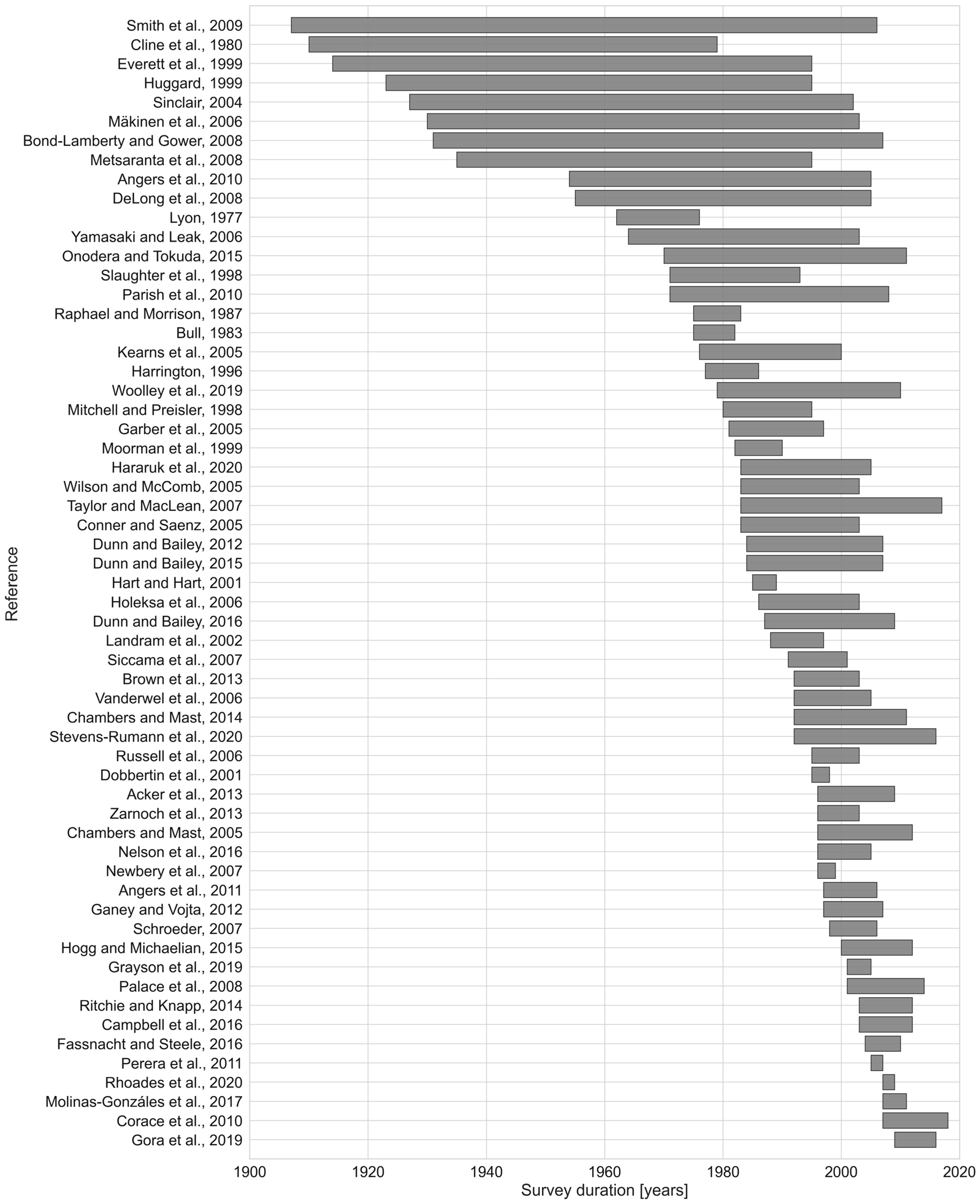
2.1.1. Literature Search and Data Extraction

We searched titles, keywords and abstracts in all databases of the Web of Science on the 11 November 2021, using the following combination of keywords and search operators: snag fall OR snag persistence OR snag fall rate* OR snag* longevity OR snag survival OR time from death to fall OR time since death snag OR snag survival OR standing snags dynamics OR dead wood abundance snag OR snag characteristics. We considered three types of studies applicable to derive the mean time to fall (MTF), ordered by increasing complexity:

• Studies based on counts of dead standing trees (DSTs) not distinguishing size classes;
• Studies based on counts of DSTs distinguished by size classes;
• Studies based on volume/dry mass of DSTs.

The MTF based on counts are hereinafter referred to as MTF_count (Section 2.3.1). For studies of DST counts distinguishing size classes, we calculated MTF_count and MTF_size, wherein the latter incorporates the total DST mass at time of death (Section 2.3.2), whereas the MTF based on volume/dry mass is referred to as MTF_m (Section 2.3.3).

The search resulted in 203 papers, of which 16 were duplicates, and we added another 7 papers from reference lists (Figure 1). We screened the abstracts of 194 papers and excluded 109 papers because they did not contain relevant data. Therefore, we assessed the full text of 85 publications, of which we excluded 15 because they were located at the same study location, had irrelevant outcomes or missed crucial data. In total, 70 papers were included in the analysis [7,10,22,26,28,45,48,49,50,51,52,53,54,55,56,57,58,59,60,61,62,63,64,65,66,67,68,69,70,71,72,73,74,75,76,77,78,79,80,81,82,83,84,85,86,87,88,89,90,91,92,93,94,95,96,97,98,99,100,101,102,103,104,105,106,107,108,109,110,111]. From each paper, we collected data that could be converted into the MTF (Section 2.2).

We assembled site geographical information such as country, region, site name and site coordinates. If exact coordinates were not presented, we estimated the study locations from maps or location descriptions. However, where information about fall times was only reported for regions or countries, we treated the location as missing.

Site properties recorded from studies included forest management history, elevation, dominant mortality cause and species characteristics. Authors reporting mean site data did not present individual species information. In these cases, we recorded the dominant species and the percentage of the dominant species’ contribution to the total species mix. Species were categorized into coniferous or broadleaved plant functional types (PFTs), and we determined the dominant PFT for sites by the prevalence of coniferous or broadleaved species (>50% of all DSTs on site).

Information on tree size was recorded as the mean diameter at breast height (DBH) per site, species or species size classes (number of publications (np) = 49). For papers reporting size classes of DSTs (np = 21), we calculated the mean DBH of species or sites using the average DBH of size classes and the number of DSTs per size class. If the maximum DBH of the largest DBH class was not reported, we estimated the mean of the largest DBH class by adding the average difference between size class means and the largest size class (np = 15). For publications wherein DBH was only given for all species or sites combined (np = 9), we assumed the same DBH class distribution (np = 9) for all sites and species, while maintaining relative species contributions to the total number of trees (e.g., [113]). We evaluated this assumption using data where the DBH distribution was reported by species individually and found that the mean absolute deviation of the mean DBH at the same site was on average 4 cm for the range of DBH (12–51 cm) when we applied this simplification, which we judged to be adequate for this analysis. If DBH class distribution was not reported by the authors, we estimated species DBH class distribution from other papers or published data from databases at the same location (np = 3;

Table A1. Source publications of MTF data for which we used additional references to determine the DBH distribution. We only selected studies that were conducted at the same locations. Time frames between MTF and DBH distribution source studies [114,115,116] did not overlap for 2 of 3 studies but were started within 1–2 years of studies from which we derived the MTF [52,65,69].

MTF Source		Description	DBH Distribution Source
Reference	Survey Duration		Reference	Survey Year(s) Used
Everett et al. (1999)	1914–1995 *	Same dataset. Number of trees/DBH class and species digitized from Figure 3 in Lehmkul et al. (2003).	Lehmkuhl et al. (2003)	1914–1995 *
Garber et al. (2005)	1981–1997	Tree based data from the NAT treatment (no intervention) from the 1999 inventory to estimate mean DBH by species for which Garber reported DBH specific DST survival curves and model coefficients (category 5; Table 2). DBH classes from grouping species’ DSTs into equally sized bins. Stand density to model DBH specific MTF by species also based on Kenefic et al. (2015).	Kenefic et al. (2015)	1999
Bull (1983)	1975–1982	DBH distribution based on Table 2 in Bull (1975) which includes all species.	Bull (1975)	1973–1974

* Based on time since fire.

) that were either based on the same dataset (np = 1; [114]) or conducted within 1–2 years of the MTF studies (np = 2 [115,116]), requested data from the studies’ principal investigators (np = 3; [74,78,94]) or estimated the DBH class distribution by using published generalized stand structure parameters which were applied by the authors themselves (np = 1; [111]).

Finally, we collected information about the authors’ methodology: the number of plots, plot size, number of DSTs included in the analysis and minimum DBH of dead standing trees to be included in the survey, total survey duration and re-measurement interval and the model form used by the authors to describe the fraction of DSTs remaining over time.

2.1.2. Ancillary Data

For each study site, we collected a range of supplementary variables considered important for decomposition: climate (temperature, soil moisture) and wood traits (substrate quality, tree size;

Table 1. Multiple linear regression covariates grouped by their effect on decomposition: climate (temperature, moisture) and wood traits (substrate quality, tree size) to avoid correlations of |r| > 0.7 between variables and thereby multicollinearity in regression models [125]. MAT—Mean annual air temperature. MAP—Mean annual precipitation. DBH—Diameter at breast height. DBH refers to the mean site and mean species DBH at site and species level, respectively (Figure 2). * PFT (plant functional type) is 1 if sites were dominated by coniferous trees (>50% trees) or 0 if sites were dominated by broadleaved trees. For species, PFT classified species as coniferous or broadleaved. † Variables only available for subset of observations at species level and analyzed separately. ‡ Variables only for a subset at both site and species level and analyzed separately.

Climate		Wood Traits
Temperature	Moisture	Substrate Quality	Tree Size
MAT	MAP	PFT *	DBH
MATsoil	Soil water ‡	Wood durability †
	Soil water max ‡

). We extracted mean annual air temperature (MAT) and mean annual precipitation (MAP) for each study site with reported location coordinates from three commonly used global gridded climate datasets of different resolutions and time periods. We aggregated six-hourly CRUNCEPv7 data (1901–2016; [117]) with a resolution of 0.5° × 0.5° over the standardized reference period, 1981–2010 (CRUclim), and over the observation period of each study if start and end year were reported (CRUobs; np = 56; Figure A1). We treated extensions of the observation periods beyond the temporal coverage of CRUNCEPv7 as missing data (np = 1; [100]) and used CRUclim for studies with location coordinates but missing information about the observation period (np = 9). We used bioclimatic data of different standardized reference periods of MAT and MAP from CHELSA (Climatologies at high resolution for the Earth’s land surface areas) aggregated for 1981–2010 at 30 arc seconds [118,119] and WorldClim2 at 10 m and 30 arc seconds over the standardized reference period, 1970–2000 [120]. Mean annual soil temperature (MATsoil) of the topsoil (0–5 cm) was extracted from the SoilTemp maps version 1 [121,122]. Mean and maximum annual soil water saturation of the topsoil layer (0–30 cm depth) covering the standardized reference period 1970–2014 were collected from SOIL-WATERGRIDS [123,124].

To capture wood substrate quality by species, we calculated species-specific mean values over all species entries for stem carbon content (mg/g) from the TRY Database [126]. We also used a wood durability dataset which rates species’ wood microbial and insect decay resistance from zero (not durable/non-resistant) to four (very durable/resistant) [40,41,42]. We used the methodology described by Oberle et al. [42] to fill gaps in the dataset. Wood durability could only be used in combination with species-specific MTFs (Supplementary Data S1).

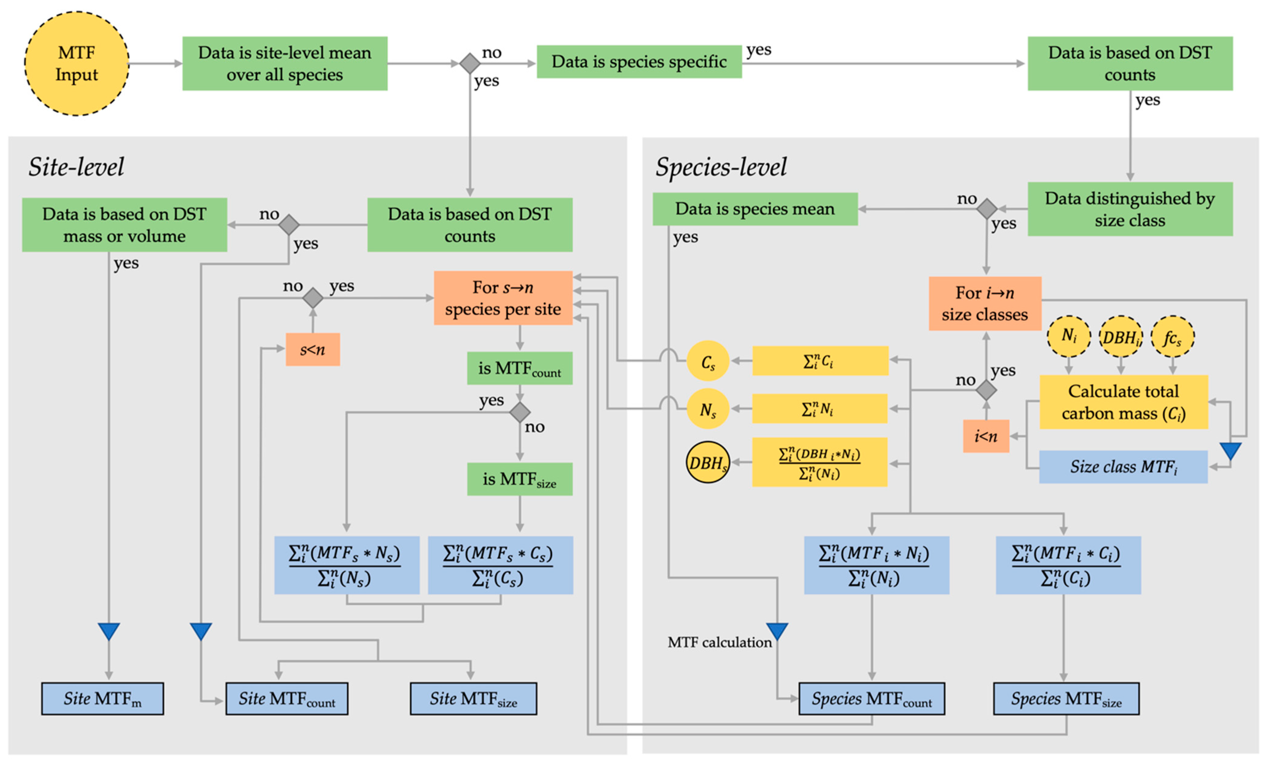
2.2. Primary MTF Calculation and Pre-Processing of Collected Data

The mean time to fall (MTF) of DSTs is analogous to the mean residence time (MRT). The MRT is based on the individual residence times of DSTs, which form a frequency–time distribution, the mean of which is the MRT. In cases of the single exponential model presented by Olson [127],

$$f=e^{-k\ast td}$$

(1)

where k is the rate constant describing the fraction of DSTs falling, td is time since death in years and f is the fraction of DSTs remaining standing over time, the MRT and MTF can be calculated as the following:

$$MTF=MRT=\frac{1}{k}$$

(2)

However, for studies using model forms other than the single exponential model, we approximated the MTF from interpolated time series of the fraction of DSTs remaining with time since death until 99% of DSTs had fallen, as follows:

$$MTF\approx {{\displaystyle \sum }}_{i=0}^n\left[\mathsf{∆}td\ast f_i\right]$$

(3)

where ∆td = 0.001 is the time step of the interpolation in years, f is the fraction of DSTs remaining for 0.01 ≤ f ≤ 1 and n is the number of time steps required such that $f_n\approx 0.01$. We evaluated the possible prediction bias of defining time series of the fraction of DSTs for 0.01 ≤ f ≤ 1 compared to the analytical solution in Equation (2) for different k and found that, independent of the order of magnitude of k, prediction bias was ~1% (Figure A2). We processed the collected data such that we could calculate the MTF using either Equation (2) or Equation (3), which required pre-processing depending on the type of the reported data (

Table 2. Reporting types, corresponding key assumptions and number of papers included from the literature search. Reporting types 1–4 were based on Olson [70]. Survival curves were based on statistical survival analysis using different model forms, persistence curves used different model forms fitted to the data and data simply reporting the number of DSTs remaining at each census interval. Number of papers (n_p) is not equal to papers in Figure 1 because two publications used different methods. Reporting types by reference are reported in Supplementary Data S1.

	Reporting Type	Key Assumption	np
1	mean residence time	steady state	4
2	decay constant k	single negative exponential decay	12
3	mean annual fall rate (F, % y−1)		8
4	single observations of percent of dead standing tree count, volume or mass remaining; single estimate of the probability to remain after n years (f)		15
5	survival or persistence curves; data	other	33

).

Studies were considered applicable if they reported information about how long dead trees remained standing since time of death, DST fall rates or the probability of DSTs to remain standing since time of death using one of the reporting types in Table 2. We considered the probability of one DST to remain standing at time t to be the fraction of the DST population to remain at time t. The MTF reporting types in Table 2 can be separated into two groups: (1) studies using single exponential decay dynamics originally presented by Olson ([70]; categories 1–4) and (2) studies publishing DST persistence over time by presenting raw data or persistence curves based on different models or statistical techniques (category 5). For the latter group to be considered applicable, we required that the data could be expressed as a fraction of dead tree count or volume/mass still standing since time of death. If authors reported the fraction of DSTs remaining over time, we required that at the end of the observation period DST fall had started. However, in cases where DST fall had started for all tree size classes except for the largest tree size class, we assumed the mean time to fall of the largest size class to be equal to the next smallest size class (n_p = 1; one species [96]).

Estimates of reporting type 1 and 2 did not require any pre-processing. Estimates based on reporting types 3 and 4 were converted to the fall rate k using the single exponential model (Equation (1) [70]). In cases where annual percentage fall rates (category 3, Table 2; F% y⁻¹) were reported, we assumed Equation (1) applied and converted fall rates to k as follows:

$$k=ln\left(-\frac{100}{F-100}\right)$$

(4)

In cases where the fraction of DSTs remaining after a fixed observation period or half-lives were reported, we assumed single exponential decline following Equation (1) and converted the observations to annual fall rates:

$$F=100\ast (1-f^{\frac{1}{td}})$$

(5)

If authors reported no more dead standing trees at time since death (n_p = 6), we assumed that time since death was equal to the time when ~99% of DST had fallen (t₉₉), which can be approximated as $t_{99}=\frac{5}{k}$, where t₉₉ using Equation (1) results in $f\left(t_{99}\right)=0.0067\approx 1\%$ for k > 0. Therefore, we approximated k in these cases as $k=\frac{5}{t_{99}}$. We tested the sensitivity of late observations on the estimated MTF using a range of k and time intervals of 5–15 years post t₉₉. Values of the MTF that were observed post t₉₉ differed 1–3 years in absolute terms from k-based MTF, independent of the order of magnitude of k. Therefore, the percentage bias to actual MTF decreased with increasing MTF, approaching 0 (Figure A3). In our collected data, mean survey intervals were 4 years with a maximum of 12.5 years; therefore, the probable mean prediction bias using t₉₉ to estimate k is <25% of the MTF or 1 year in absolute terms (Figure A3).

If authors, in addition to DST fall rates, reported lag times, i.e., the time before dead trees started falling, we assumed no falling of dead trees during that period and used Equations (1) and (4) to generate time series of the fraction of DSTs remaining since time of death and linearly interpolated between points such that ∆td = 0.001 (cf. Equation (3)). Lag times then preceded time series of the fraction of DSTs, which were then processed further to MTF using Equation (3).

The reporting type category 5 consisted of persistence or survival curves of DST counts or volume/mass based on fitted models (including generalized mixed linear models, logistic models, Weibull functions and survival analysis) applied to field data or tree counts by time since death. We first digitized the published data [128] and transformed the data to fractions of DST counts or mass/volume remaining over time, and linearly interpolated between points (∆td = 0.001) to yield time series of the fraction of DSTs remaining since time of death. If data were collected at discrete intervals, we assumed that dead trees had fallen at the midpoint between measurement intervals. In cases where the data indicated that >10% DSTs were still standing at the end of the study period (n_p = 9), we fitted a logistic model of the following form:

$$f=\frac{1}{a+e^{c\ast \left(td-b\right)}}$$

(6)

where a, b and c are fitted parameters and f is the fraction of DSTs remaining at time since death (td [years]). The resulting time series of the fraction of DSTs remaining was then generated for 0.01 ≤ f ≤ 1, i.e., until 1% of DSTs were remaining. Rate constants (k) and time series of the fraction of DSTs remaining since times of death were then processed to estimates of MTF using Equations (2) and (3).

2.3. MTF Calculation at Site and Species Level

We calculated the MTF at site and species levels, wherein site-level MTF is the mean site MTF and species-level MTF is the MTF averaged per individual species per site (Figure 2). We report all MTF values at site and species levels, as well as covariates and data citations, in Supplementary Data S1. Site-level MTFs were based on reported mean values by authors, or we aggregated all species-specific MTFs per site by weighing species’ MTFs by the number of DSTs of each species (Figure 2). Whilst we aimed to test species-level differences in MTF, not all studies report this level of information; thus, to maximize the geographic representation and overall sample size, we also investigated the site-level values. Furthermore, site- and species-level MTFs represent two levels of aggregation, and presenting both in this study enables assessment of how the level of aggregation might impact MTF predictions.

Based on rate constants (k) and the time series of the fraction of DST counts remaining over time, we determined the mean time for DSTs to fall (MTF_count; Figure 2; c.f. Section 2.2). When tree count data distinguished by size classes was available, we also calculated MTF_size, which better accounts for size effects on mean time to fall than MTF_count. When DST volume or mass was reported with time since death (n_p = 8), we determined MTF_m, which also incorporates mass loss with time since death. A total of 21 studies reported size classes and the remaining 41 studies reported tree counts at site or species levels. We found significant linear relationships (p < 0.05) between MTF_count and MTF_size at site and species levels (Figure A4), as well as when we separated species data by plant functional type (PFT; coniferous and broadleaved; Figure A5) using ordinary least squares regression. The linear regressions were forced through zero [129] and bootstrapped to estimate the 95% confidence interval of the mean slope using repeated sampling with replacement (n = 1000). We used site (Figure A4a) and plant-functional-type-specific (Figure A5) regression slopes to convert MTF_count to MTF_size for 44 studies at site and species levels, respectively.

2.3.1. Studies Based on Counts of Dead Standing Trees (MTF_count)

Dead standing tree (DST) fall rate constants (k) were converted to the mean time to fall (MTF_count) by taking the inverse of k (Equation (2)). For time series of digitized data in reporting category 5 (Table 2), which included site, species and species-size-class-specific data (Figure 2), MTF_count was calculated using Equation (3). Where we had size class data, we determined species-level MTF_count from species size class’ MTF_count by taking a weighted average using the number of dead standing trees of these size classes and similarly determined a mean site MTF_count by weighting individual species on site by their number of DSTs (Figure 2). We consider these mean-species and mean-site MTF_counts as equivalent to the estimates calculated from studies that did not distinguish by size classes (Figure 2).

2.3.2. Studies Based on Counts of Dead Standing Trees Distinguished by Size Classes (MTF_size)

For studies reporting DST fractions distinguished by size classes, we determined MTF_count as described in the previous section and then aggregated MTF_count by taking a weighted mean of size-class-specific MTF_count and the respective total carbon mass of each size class (C_i; Figure 2) at time of death to determine MTF_size by species and site, which we consider a better representation of the average time carbon remains in DSTs than MTF_count.

To determine MTF_size, we assumed DSTs to be whole trees at time of death and estimated total dry weight biomass of size classes from the mean DBH per size class using the generalized biomass equation and species-group-specific parameters presented by Chojnacky et al. [130]. We then applied species-specific mean carbon concentrations from the TRY Database [126] to estimate standing dead wood carbon of the average tree for each size class [131]. Using the number of DSTs within size classes per species, we estimated total species carbon mass at time of death for each site (C_s; Figure 2). We also used the mean DBH of species’ size classes (DBH_i; Figure 2) and the number of trees per size class (N_i; Figure 2) to calculate the mean weighted site-level DBH (DBH_s; Figure 2).

2.3.3. Studies Based on Volume/Dry Mass of the Dead Standing Trees (MTF_m)

Studies based on the volume/dry mass of DSTs report their findings as mean residence times of DST volume/dry mass (category 1, Table 2, e.g., Chambers et al., Palace et al., Gora et al. [22,95,132]) or as the mass/volume of DSTs remaining over time (category 5, Table 2, e.g., Akala [103]). These studies incorporate density loss due to decomposition either by measuring wood density of DSTs in decay classes [103] or by applying the steady-state assumption to measurements of influx into the dead standing wood pool (mortality), size of the standing dead wood pool and transfer of standing dead wood mass to downed woody debris [22]. Therefore, the studies in these categories incorporate mass loss and could be considered the closest estimate of the mean residence time of biomass in standing dead wood. None of the studies, however, converted their dry mass to carbon, and therefore we call the mean time to fall based on these studies MTF_m.

2.4. Relationships of MTF to Explanatory Variables

We analyzed the MTF of DST at site and species levels separately and distinguished between MTF_count and MTF_size due to autocorrelation caused by the conversion from MTF_count to MTF_size (Figure A4 and Figure A5). Since our aim in this study is to identify large-scale dynamics of DST fall, we considered all species per site as individual data points described by their plant functional type (PFT) and tree size (DBH), to find relationships that explain the species-level MTF on a generalized level.

All MTF data were log-transformed to meet the requirements of a normal distribution for statistical tests and linear regressions. We classified sites and species by their dominant mortality causes: fire (M_Fire), insects and associated fungi (M_Insects) or other mortality (M_Other), as well as by plant functional type (PFT) and if forests had a reported history of management or not. If authors had indicated that both managed and unmanaged forest stands had been used in their analysis, we treated their data as managed. Not-reported categories were treated as missing.

At site and species levels, we first tested whether the log-transformed MTF significantly differed (p < 0.05) between mortality causes (M_Fire, M_Insects, M_Other), management or PFT using pair-wise statistical testing, assuming independent samples. We confirmed the homogeneity of variances using the Levene test before performing t-tests (scipy v1.7.3 [129]), or if the prerequisite of homogeneity of variances was not fulfilled, we performed a Kruskal–Wallis test (scipy v1.7.3 [129]), to determine whether groups differed significantly from each other.

Next, we trained regression models to further explore the drivers and control for differences in background climate. To ensure comparability between them, we identified the largest data subset including no missing data across variable groups, shown in Table 1, and management. Wood durability was only available for a subset of our data, and therefore we used PFTs as proxies for wood substrate quality differences [37] for 64 and 107 data points at site and species levels, respectively. We grouped potential covariates by whether they described the temperature, moisture availability or substrate quality effect on decomposition (Table 1) to keep correlations between groups of variables to below |r| < 0.7 [125], and tested all possible variable combinations between groups using ordinary least squares multiple linear regression (statsmodels v0.13.2 [133]). We treated all covariates as fixed effects because interaction effects between covariates shown in Table 1, mortality cause and management, led to non-valid regression models, as judged by the variance inflation factor (VIF ≥ 5). To ensure homoscedasticity of model residuals, we performed post hoc White tests (scipy v1.7.3 [129], p < 0.05) and excluded all models that did not pass the test. If a variable combination included MAT or MAP, we determined the best model for each climate dataset (n = 5, CRU_clim, CRU_obs, CHELSA_30s, WorldClim_30s and WorldClim_10m).

We retained models when covariates were significant, with p < 0.01, and ranked models by the difference in Akaike Information Criterion (∆AIC [134]) with the model with lowest AIC. A ∆AIC of 2 is often used as a rule of thumb to identify models that are indistinguishable from each other. However, Richards [135] showed that there is 32% chance of the best model having a ∆AIC of more than 2, but this chance is reduced to 17%–5% when ∆AIC thresholds of 4–7 are used; therefore, we retain models with ∆AIC < 6. We then sorted and ranked models by ∆AIC, adjusted the coefficient of determination (R2) and the root-mean-squared error (RMSE) and preferred models with a lower number of covariates and lower RMSEs. Additionally, we standardized covariates to determine their relative effect on MTFs using their standard score and error.

We tested regression results for highly influential data points using Cook’s distance (statsmodels v0.13.2 [133]) and checked the data points with the highest leverage on regressions. Two data points with the highest leverage on species-level regressions were removed from the analysis because they were anomalous in several respects. Specifically, for both references, DSTs had died by fire, with one reference reporting re-burnt DST data [85], and for the other, the data was based on patches of DSTs with varying levels of retained basal area within an otherwise completely salvage-logged landscape [97], which was not reported by any other publication included in this study.

Using dominant mortality cause as a covariate in regression models did not lead to valid regression models (see above); therefore, we tested whether grouping data by mortality would result in a different model selection. We did not have enough data to consider M_Insects individually, and therefore tested whether M_Insects inclusion or exclusion would change resulting regression models. We tested 4 mortality groups: M_All, which included all mortality causes, M_Fire, which only included sites and species where trees died by fire, M_NoFire, which includes sites and species where the mortality was caused by insects and other causes, and M_Other, where insect and fire mortality were removed. To simplify the analysis, we analyzed M_Fire, M_NoFire, M_Other results only for MAT and MAP based on the best-performing climate dataset for M_All, for which we had the highest data availability.

The substrate quality variable wood durability was not available for all data points of the species subset; we therefore compared wood durability with plant functional type for the mortality cause where we had found a significant relationship with PFT and CRU_obs. We determined the best regression model for the substrate quality subset following the model selection method outlined above.

As a last step, we used the species regression model of the mortality group that excludes fire as well as insects (M_Other) to estimate the MTF at our 2 tropical sites (Figure 3) for which the DBH was missing and compare this with the reported MTF at these sites.

3. Results

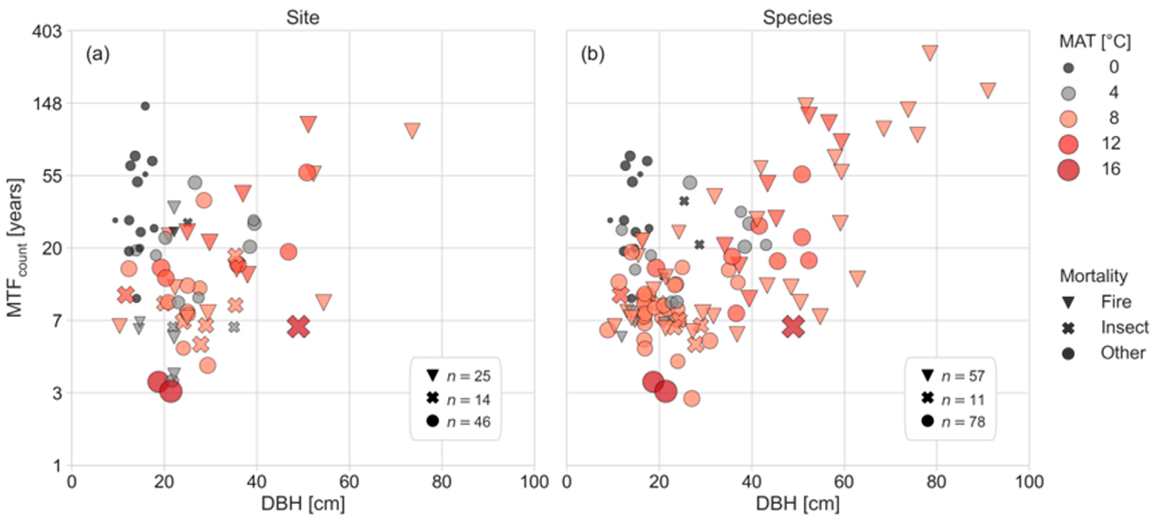
3.1. Overview the of Mean Time to Fall (MTF) for Dead Standing Trees (DST)

Of the 70 applicable publications identified (Figure 1,

Table 3. Overview of the MTF database (Supplementary Data S1) by continent for site and species levels. n_p is the number of publications. “All” is the number of sites or species (n). Plant functional type (PFT) is the fraction of sites dominated by conifers and the fraction of species that are coniferous at site and species levels, respectively. The percentage of sites and species impacted by fire mortality and management is presented. DBH is the mean site- or species-level DBH by continent. Values include regional studies which did not report exact locations but where we could assign continents based on countries. Missing values omitted. Regression analysis presented in Table 4 and Table 5 based on the largest data subset where MAT, PFT and DBH were reported (cf. Section 2.4).

Continent	np	Site					Species
		All	PFT	Mortality	Managed	DBH	All	PFT	Mortality	Managed	DBH
			Conifer	Fire				Conifer	Fire
	(n)	(n)	(%)	(%)	(%)	(cm)	(n)	(%)	(%)	(%)	(cm)
North America	57	113	84.1	25.7	15.9	23.2	153	68.6	40.5	22.2	26.9
Europe	10	15	93.3	13.3	33.3	26.2	17	70.6	11.8	23.5	23.6
Asia	1	1	100	0	0	27.6	7	28.6	0	0	26.4
Oceania	1	1	0	0	0	-	2	0	0	0	-
South America	1	1	0	0	0	-	-	-	-	-	-
All	70	131.0	84.0	23.7	17.6	23.5	179.0	66.5	35.8	24.1	26.8

), 80% reported data from North American sites, followed by Europe (16%), Asia (1.4%), South America (1.4%) and Oceania (1.4%), but we did not find any studies of DST fall in Africa (Figure 3a). Study locations were predominantly classified as taiga and temperate deciduous forest or grassland, with only two sites located in tropical forests based on the Whittaker biome model (Figure 3b). The most abundant coniferous tree families were spruce (Picea spp.), pine (Pinus spp.) and fir (Abies spp.), and broadleaved trees were mainly birch (Betula spp.) and poplar (Populus spp.).

For the entire dataset, the average species’ MTF_count was 48, 13 and 19 years for DSTs that died by fire, insects and other causes, respectively. When we accounted for the total DST carbon mass at time of death to calculate MTF_size (Figure 2), we found about two times longer standing times compared to count-based MTFs (Figure A4), indicating that residence times for standing carbon might not be well represented by MTF_count. The longer standing times for MTF_size compared to MTF_count were driven predominantly by coniferous species, for which we predicted 48% longer standing times when we accounted for tree size. However, broadleaved species only stood 23% longer when we accounted for tree size, which is caused by a smaller average size of broadleaved DSTs compared to coniferous trees in our dataset.

MTF data characterized by plant functional type (PFT) representing broadleaved and coniferous trees’ mortality cause (fire, insects and other causes) as well as management were unevenly distributed in the dataset (Figure 4;

Table A2. Covariate mean and range of multiple linear regressions for mortality groups at site and species levels distinguished by management presence which we report as managed “Yes” or “No”. MAT based on CRU_obs. The PFT value represents the fraction of sites dominated by conifers and species categorized as coniferous at site and species levels, respectively. Number of observations (N_obs) is the number of data points by mortality group used to derive mean and range of covariates.

	Mortality	Managed	MTFcount [Years]	DBH [cm]	MAT [°C]	PFT [-]	Nobs
Site	All	No	22.0 (4.0–148.0)	25.5 (9.4–73.6)	3.95 (−3.1–9.8)	0.93	46
		Yes	9.0 (3.0–49.0)	27.52 (14.7–49.0)	6.66 (−0.3–19.2)	0.89	18
	Fire	No	20.0 (4.0–110.0)	32.1 (14.5–73.6)	5.81 (0.3–8.5)	1.0	16
		Yes	7.0 (7.0–7.0)	14.73 (14.7–14.7)	0.9 (0.9–0.9)	1.0	1
	Insects	No	10.0 (7.0–18.0)	27.52 (11.7–35.4)	5.82 (1.0–9.1)	0.80	5
		Yes	9.0 (7.0–27.0)	29.81 (21.9–49.0)	6.8 (−0.3–19.2)	1.0	5
	No Fire	No	22.0 (7.0–148.0)	21.98 (9.4–50.9)	2.96 (−3.1–9.8)	0.90	30
		Yes	9.0 (3.0–49.0)	28.27 (18.7–49.0)	7.0 (−0.3–19.2)	0.88	17
	Other	No	26.0 (8.0–148.0)	20.87 (9.4–50.9)	2.38 (−3.1–9.8)	0.92	25
		Yes	9.0 (3.0–49.0)	27.63 (18.7–46.9)	7.08 (3.1–18.0)	0.83	12
Species	All	No	22.0 (4.0–299.0)	30.44 (8.9–91.1)	4.93 (−3.1–9.8)	0.87	75
		Yes	9.0 (2.0–49.0)	25.69 (14.7–52.4)	6.51 (−0.3–19.2)	0.53	32
	Fire	No	28.0 (6.0–299.0)	40.18 (11.9–91.1)	6.34 (1.3–8.5)	0.97	36
		Yes	7.0 (7.0–7.0)	14.73 (14.7–14.7)	0.9 (0.9–0.9)	1.0	1
	Insects	No	10.0 (9.0–11.0)	15.84 (11.7–20.0)	7.8 (6.5–9.1)	0.5	2
		Yes	11.0 (7.0–37.0)	28.68 (21.1–49.0)	5.71 (−0.3–19.2)	1.0	7
	No Fire	No	18.0 (4.0–74.0)	21.44 (8.9–50.9)	3.64 (−3.1–9.8)	0.77	39
		Yes	9.0 (2.0–49.0)	26.04 (16.6–52.4)	6.69 (−0.3–19.2)	0.52	31
	Other	No	18.0 (4.0–74.0)	21.74 (8.9–50.9)	3.41 (−3.1–9.8)	0.78	37
		Yes	9.0 (2.0–49.0)	25.27 (16.6–52.4)	6.98 (3.1–18.0)	0.38	24

), increasing difficulty for statistical inference. However, when testing for statistically significant differences between categories, we found that site-level MTF_count and MTF_size differed significantly between sites with a known management history and unmanaged or old-growth sites, but not between conifer- and broadleaf-dominated sites, or for sites where mortality of the DSTs was caused by fire versus other causes (Figure 4a; t-test, p < 0.05).

We refer to the MTF of species on a site as species-level MTF (Figure 2), which is characterized by its mean DBH and PFT and site properties such as mortality cause, management and climate. We found statistically significant differences between the species-level MTF of coniferous and broadleaved DSTs (Figure 4b; t-test, p < 0.001; Table A2), DSTs that died by fire or other causes (Kruskal–Wallis, p < 0.001; Table A2) and DSTs from managed and unmanaged sites (t-test, p < 0.001; Table A2).

The highest MTFs and tree sizes were generally connected to mortality by fire and the coniferous PFT (Figure 4, Figure 5 and Figure A8; Table A2). However, when we used pair-wise statistical tests to test mortality caused by insects (M_Insects) and other mortality causes (M_Other) against fire mortality (M_Fire), we found no significant difference (p < 0.05; Figure A6). There were, however, significant differences between the species’ MTFs that died by insect attack (M_Insects) and other causes (M_Other; Figure A6), where M_Insects had a lower mean and range than M_Other, suggesting that pooling mortality causes might obscure relationships of the MTF with mortality cause.

Generally, site-level MTFs and species-specific MTFs increased linearly with increasing tree size (DBH) after log transformation, whereas MTFs at MATs below 2 °C diverged markedly from this trend, showing high MTFs for small tree sizes (Figure 5).

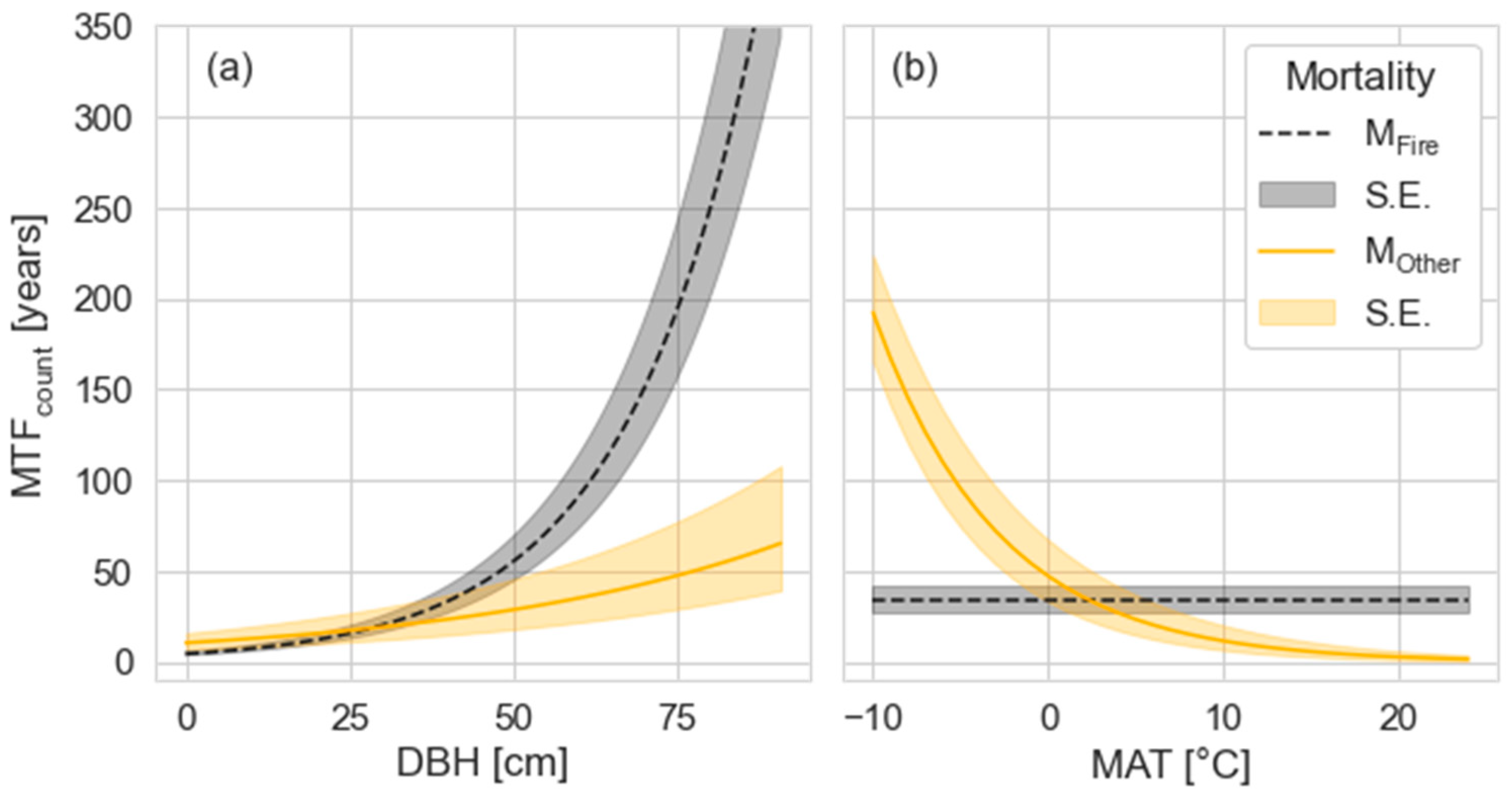
3.2. Drivers of Mean Time to Fall for Dead Standing Trees

We analyzed the drivers of the MTF of DSTs using multiple linear regression models using variables linked to decomposition and species traits (Table 1). We further distinguished by mortality group by way of analyzing all mortality causes together (M_All), fire mortality (M_Fire), mortality caused by other causes than fire including insects (M_NoFire) and other causes (M_Other). Species-level regression models of the MTF explained more variation than site-level models (

Table 5. Species- and site-level coefficients and standard errors of best models for log-transformed MTF_count and MTF_size by mortality groups for models presented in Table 4. PFT categorizes sites into dominated by coniferous (PFT = 1) or broadleaved species (PFT = 0) and species whether they are coniferous (PFT = 1) or broadleaved (PFT = 0). Management indicated whether sites had a known history of management (management = 1) or were reported as unmanaged or old growth (management = 0). Covariate mean and range at site and species levels and by mortality group displayed in Table A2.

	Mortality	Intercept		DBH		MAT		PFT		Managed
		Count	Size	Count	Size	Count	Size	Count	Size	Count	Size
Site	All	2.64 (0.22)	3.25 (0.23)	0.03 (0.01)	0.03 (0.01)	−0.09 (0.02)	−0.11 (0.02)	-	-	−0.69 (0.21)	−0.78 (0.22)
	Fire	1.44 (0.37)	2.13 (0.41)	0.05 (0.01)	0.05 (0.01)	-	-	-	-	-	-
	No Fire	3.25 (0.15)	3.90 (0.16)	-	-	−0.11 (0.02)	−0.13 (0.02)	-	-	-	-
	Other	3.40 (0.16)	4.07 (0.17)	-	-	−0.12 (0.03)	−0.15 (0.03)	-	-	-	-
Species	All	2.40 (0.13)	2.71 (0.15)	0.04 (0.00)	0.04 (0.00)	−0.12 (0.02)	−0.13 (0.02)	-	-	−0.45 (0.13)	−0.49 (0.15)
	Fire	1.51 (0.22)	1.83 (0.25)	0.05 (0.00)	0.05 (0.01)	-	-	-	-	-	-
	No Fire	2.52 (0.16)	2.83 (0.18)	0.02 (0.01)	0.02 (0.01)	−0.13 (0.02)	−0.14 (0.02)	0.44 (0.14)	0.43 (0.15)	-	-
	Other	2.54 (0.17)	2.87 (0.19)	0.02 (0.01)	0.02 (0.01)	−0.14 (0.02)	−0.15 (0.02)	0.52 (0.14)	0.52 (0.15)	-	-

,

Table A3. Best performing multiple linear regression models for data including all mortality causes (M_Other) at site (n = 37) and species-level (n = 107) for log-transformed MTF_count and MTF_size (Table 4 and Table A4) for 6 different climate datasets (p < 0.01). CRU_obs is the mean over the observation period while CRU_clim, CHELSA_30s and WorldClim2_30s and WorldClim_10m are based on climate periods. R² is the coefficient of determination and RMSE is the root mean squared error in years.

	Model	Climate	MTFcount		MTFsize
			R2	RMSE	R2	RMSE
Site	MAT + DBH + Managed	CRUclim	0.34	23.7	0.40	49.6
		CRUobs	0.36	23.4	0.42	49.3
		CHELSA30s	0.30	24.6	0.35	51.2
		WorldClim30s	0.34	24.5	0.40	51.2
		WorldClim10m	0.32	24.5	0.39	50.9
	MATSoil + DBH + Managed	SoilTemps	0.34	24.4	0.40	51.1
Species	MAT + DBH + Managed	CRUclim	0.61	26.0	0.57	44.0
		CRUobs	0.61	26.0	0.59	44.0
		CHELSA30s	0.58	26.3	0.57	43.3
		WorldClim30s	0.58	27.3	0.56	46.4
		WorldClim10m	0.55	27.4	0.54	45.4
	MATsoil + DBH + Managed	SoilTemps	0.62	27.4	0.59	45.9

and

Table A4. Multiple linear regression result for log-transformed MTF_count and MTF_size at site and species levels for the best performing variable combinations with significant parameters (p < 0.01) and ∆AIC < 6, ranked by R² and RMSE. Selected model shown in bold. R² is the coefficient of determination, AIC is the Akaike information criterion, ∆AIC is the difference in AIC to the best performing model and RMSE is the root mean squared error in years. N_obs is the number of observations by mortality type that included entries for MAT, tree size (DBH), management and plant functional type (PFT).

	Mortality Group	Model	R2		∆AIC		RMSE		Nobs	Climate
			Count	Size	Count	Size	Count	Size
Site	All	MAT + DBH + Managed	0.36	0.42	0	0	23.4	49.2	64	CRUobs
		MATsoil + DBH + Managed	0.34	0.40	1.6	1.3	24.4	51.1		-
	Fire	DBH	0.40	0.29	0	0	20.8	54.0	17	-
	No Fire	MATSoil	0.32	0.38	0	0	23.9	47.1	47	-
		MAT	0.32	0.37	0.1	0.8	23.0	45.0		CRUobs
	Other	MATSoil	0.37	0.46	0	0	25.9	51.1	37	-
		MAT	0.36	0.43	1.5	1.9	24.4	47.8		CRUobs
Species	All	MATSoil + DBH + Managed	0.62	0.59	0	0.2	26.8	46.0	107
		MAT + DBH + Managed	0.61	0.59	3.6	0	26.0	44.0		CRU
	Fire	DBH	0.76	0.72	0	0	34.0	58.8	37	-
	No Fire	MAT + DBH + PFT	0.54	0.54	0	0	12.4	18.8	70	CRUobs
		MAT + PFT	0.49	-	5.6	-	12.4	-		CRUobs
	Other	MAT + DBH + PFT	0.58	0.58	0	0	12.8	19.3	61	CRUobs

). DSTs that died by fire (M_Fire) generally showed the best-performing models and explained more variation than other mortality groups. Prediction errors (RMSEs) for MTF_size were a factor of ~2 higher than RMSEs of MTF_count (

Table 4. Best models for species and site by mortality group for log-transformed MTF_count and MTF_size. All models and covariates significant at p < 0.01. Corresponding coefficient values of the covariates are specified in Table 5. Coefficient of determination (R²) and root-mean-squared error RMSE (years) and number of observations (N_obs) as well as climate dataset for MAT. Covariate mean and range at site and species levels and by mortality group displayed in Table A2.

	Nobs	Mortality	Model	R2		RMSE		Climate
				Count	Size	Count	Size
Site	64	All	MAT + DBH + Managed	0.36	0.42	23.4	49.2	CRUobs
	17	Fire	DBH	0.54	0.47	21.0	54.9	-
	47	No Fire	MAT	0.32	0.37	23.0	45.0	CRUobs
	37	Other	MAT	0.36	0.43	24.4	47.8	CRUobs
Species	107	All	MAT + DBH + Managed	0.61	0.60	25.9	43.9	CRU
	37	Fire	DBH	0.70	0.65	38.4	67.8	-
	70	No Fire	MAT + DBH + PFT	0.54	0.54	12.4	18.8	CRUobs
	61	Other	MAT + DBH + PFT	0.58	0.58	12.5	19.0	CRUobs

), corresponding to the relative differences in regression slope in Figure A4.

MAT had a negative effect on the MTF across site and species levels (Table 4 and Table 5, Figure 6) and was included as a covariate in all site- and species-level mortality models except for DSTs that died by fire (M_Fire). Mean annual temperature (MAT) from CRU (CRU_clim, CRU_obs) and MAT of the soil (MAT_Soil; Table A3; Figure A7) explained similar levels of variance, but explained more variance compared to other climate datasets for both MTF_count and MTF_size. Models including MAT of the soil (MAT_Soil) explained similar levels of variance to MAT over the observation period (CRU_obs) but consistently showed higher RMSEs than models using MAT over the observation period and were therefore not selected as final models (Table A3 and Table A4).

Mean annual precipitation (MAP) had a negative influence on the MTF but was not a significant explanatory factor independent of the climate dataset. Similarly, increasing mean and maximum water saturation of the topsoil shortened the MTF, but were non-significant for the subset of data where it was available at site (n = 57) and species (n = 100) levels.

Tree size (DBH) and coniferous plant functional type (PFT) increased MTFs, but the importance of covariates differed between mortality groups (Table 4; Figure 6). Additionally, models of MTF mortality groups differed between site and species levels but not between MTF_count and MTF_size (Table 4).

3.3. Driving Factors of the MTF Differ by DST Mortality Cause

The best model wherein all causes of mortality (M_All) were considered explained MTFs at site and species levels with MAT, average DBH of DSTs and management (Table 4). Management had a negative effect on the MTF but was only selected as part of regression models when we did not distinguish by mortality causes (Table 4, Table 5 and

Table A5. Best models for DSTs that died by fire, other causes than fire (M_NoFire) and DSTs that died by other causes than fire and insects (M_Other) for the temperature range of DSTst that died by fire (M_Fire MAT subset; Table A2). M_Fire models equivalent to models shown in Table 4. Models for M_NoFire and M_Other maintain MAT as a significant predictor at site and species levels compared to models for the full temperature range covered by M_NoFire and M_Other (Table A2). Covariates significant for alpha = 0.01.

	Level	Nobs	Mortality	Model	R2		RMSE		Climate
					Count	Size	Count	Size
MFire MAT range	Site	17	Fire	DBH	0.54	0.47	21.0	54.9	-
		38	No Fire	MATSoil	0.24	0.29	25.6	50.4	-
		29	Other	MATSoil	0.22	0.28	18.7	37.6	-
	Species	37	Fire	DBH	0.70	0.65	38.4	67.8	-
		53	No Fire	MAT + DBH	0.36	0.40	12.0	18.1	CRUobs
		49	Other	MAT + DBH + PFT	0.43	-	11.4	-	CRUobs
				MAT + DBH	0.35	0.38	12.4	18.8	CRUobs

). However, for mortality caused by fire (M_Fire), managed sites were only represented by one site and species at site and species levels, respectively (Table A2); therefore, our results cannot assess a management effect on the MTF if DSTs died by fire (M_Fire).

The inclusion or exclusion of mortality by insects did not affect resulting regression models (M_NoFire and M_Other), but increased the model performance (R²), suggesting that insect mortality might confound results and should be treated separately from other DST mortality causes (Table 4).

MAT was a driver of the MTF in all models of M_All, M_NoFire and M_Other but not M_Fire. DSTs killed by fire covered a narrower temperature range than DSTs killed by other causes than fire (M_NoFire and M_Other), but when we re-ran the regression analysis at site and species levels for M_NoFire and M_Other within the M_Fire temperature range, we found that MAT remained a significant explanatory variable (Table A5). Replicating the MAT response of DSTs killed by other causes than fire (M_NoFire, M_Other) for the temperature range of M_Fire provides evidence of a robust response of the MTF to changes in MAT.

The MTF of fire-killed DSTs was instead explained by tree size (DBH), which showed an about four times larger z-score compared to DBH in MTF models for M_NoFire and M_Other at the species level (Figure 6). The large effect of DBH is caused by the very large species-level MTF and DBH values connected to fire mortality (Figure 5) that were not present for other causes of mortality (Table A2, Figure A8). Fire models at site and species levels explained the highest share of variation in the data, although these results were based on the lowest number of data points and showed the largest RMSEs (Table 4). Species-level models excluding fire mortality (M_NoFire and M_Other) had the lowest RMSEs and explained 54%–58% of the variation in MTF_count and MTF_size, using MAT, DBH and PFT as explanatory variables (Table 4). For M_NoFire and M_Other, MAT had the largest effect on the MTF as shown by its z-score (Figure 6 and Figure 7).

For mortality by other agents than fire (M_Other) where PFT was a significant covariate at the species level, we tested if wood durability was an explanatory variable where this variable was available (n = 60; Table 1). For this wood substrate quality subset and M_Other, the best-performing models were the same as those presented in Table 4, and wood durability was not included in the top models (

Table A6. Best species-level models (∆AIC < 6) for the wood quality subset (Table 1) of PFT, wood durability and C:N ratio. Covariates significant for alpha = 0.01.

	Mortality	Model	R2		∆AIC		RMSE		Nobs	Climate
			Count	Size	Count	Size	Count	Size
Species	Other	MAT + PFT + DBH	0.55	0.55	0	0	13.0	19.7	60	CRUobs
		MATSoil + DBH	-	0.50	-	5.2	-	21.8		-

).

3.4. Comparison of Regression Results with MTF_m Data from the Tropics

Two tropical sites in Panama and Brazil reported the MTF_m of DSTs, including data regarding fragmentation and decomposition, but provided no supporting site information such as mean site DBH [22]. At the sites in Panama and Brazil, MTF_m were 1.9 and 4.2 years, respectively, for a MAT of 26 °C, i.e., outside the range MAT in this study. Using the coefficients reported in Table 5 for the mortality group M_Other and a MAT of 26 °C, assuming broadleaved PFT and a mean DBH range of 80–200 cm, these models predict MTFs of ~3 and ~2 years for MTF_count and MTF_size, respectively, which is roughly consistent with the observed MTF_m estimates.

4. Discussion

We explained the mean time to fall (MTF) of dead standing trees (DSTs) using a combination of covariates considered important for woody decomposition. The most important explanatory variables were mean annual temperature (MAT) and tree size (DBH), with additional contributions from management and coniferous or broadleaved PFT. All things being equal, DSTs fell faster along gradients of increasing MAT and MAT had the largest influence on MTFs when DSTs died by other causes than fire (Figure 6 and Figure 7). However, we did not find a temperature effect on the MTF when DSTs’ mortality was caused by fire (Figure 6 and Figure 7). Larger tree size caused DSTs to stand longer, and this effect was especially strong when DSTs’ mortality cause was fire, but it influenced MTFs independently of mortality cause when we analyzed individual species’ MTFs across sites (Figure 6 and Figure 7).

We found that explaining DST fall is sensitive to aggregation level (site and species level), with species-level models explaining more variation than site-level models. Therefore, we recommend that species-level models should be used when modelling MTFs of DSTs. We further found indications that MTF drivers differed between mortality causes (Table 4, Figure 6).

4.1. Site- and Species-Level Differences

In our analysis, we considered mean site MTFs, which are means of all species on a site, and MTFs of individual species per site separately, which we refer to as site and species levels, respectively. Across mortality groups, species-level models explained 15%–29% more variation in the data compared to site-level models (Table 4), which is likely explained by site-level MTFs being aggregated over species’ MTFs (Figure 2). As such, Bradford et al. [24] showed that aggregating individual woody decomposition rates to the site level means reduced explanatory power, because within-site variation is averaged and the large-scale climate becomes more important relative to variation at the site scale, leading to overall lower explained variation.

For species-level MTFs, we explained 70 and 58% of the variation for mortality by fire (M_Fire) and other mortality (M_Other), respectively. It is possible that we can explain more variation of the MTF data compared to decomposition studies which only use climate and wood traits as predictors [137], because DST fall is also a function of the mechanical strength of the stem [42,138]. Mechanical strength, in turn, is a function of the mean DBH and a species’ or plant functional types’ decay resistance, which is typically higher in conifers than broadleaved species at the same site [37,38,39], and where tree size can even increase the decay resistance due to larger shares of heartwood and decay-resistant compounds within [15,36]. Additionally, decomposition rates are generally lower in DSTs than in wood that is in contact with the ground due to low moisture levels [15,139].

4.2. Management Effect on the MTF

Management-influenced MTFs were statistically significantly different from, and showed lower overall means than MTFs from unmanaged or old-growth sites at both site and species levels (Figure 4), where managed data points made up 28 and 29% of the data (Table A2), respectively. Management was also a significant covariate when we analyzed all mortality causes together (Table 4) and explained 10% and 4% of additional variation in the data at site and species levels, respectively. However, when we distinguished by mortality cause, management was not a driver of the MTF (Table 4). That management was not an effect when we distinguished by mortality cause either indicates that mortality cause may confound drivers of the MTF or that our dataset was too small to reliably distinguish a management effect.

Management might primarily affect MTFs through stand density and mean stand or species DBH, which was an important explanatory variable across groups and the only explanatory variable for MTFs that died by fire (Table 4, Figure 5). Individual studies have reported that management had either no effect on fall rates of DSTs [26,45] or that it accelerated fall rates [69,100,111,140], but none of these studies controlled for mortality cause. It is possible that other sites, which were reported as unmanaged, still influenced the MTF through legacy effects of management in the past, obscuring a larger management effect in the data. Importantly, the form and intensity of what is defined as management can also differ greatly. Accelerated fall rates of DSTs have been linked to increased management intensity [39,69], which we did not distinguish here. It would be valuable for future studies to investigate if management influences the MTF while controlling for tree size, mortality cause and stand density [39,44].

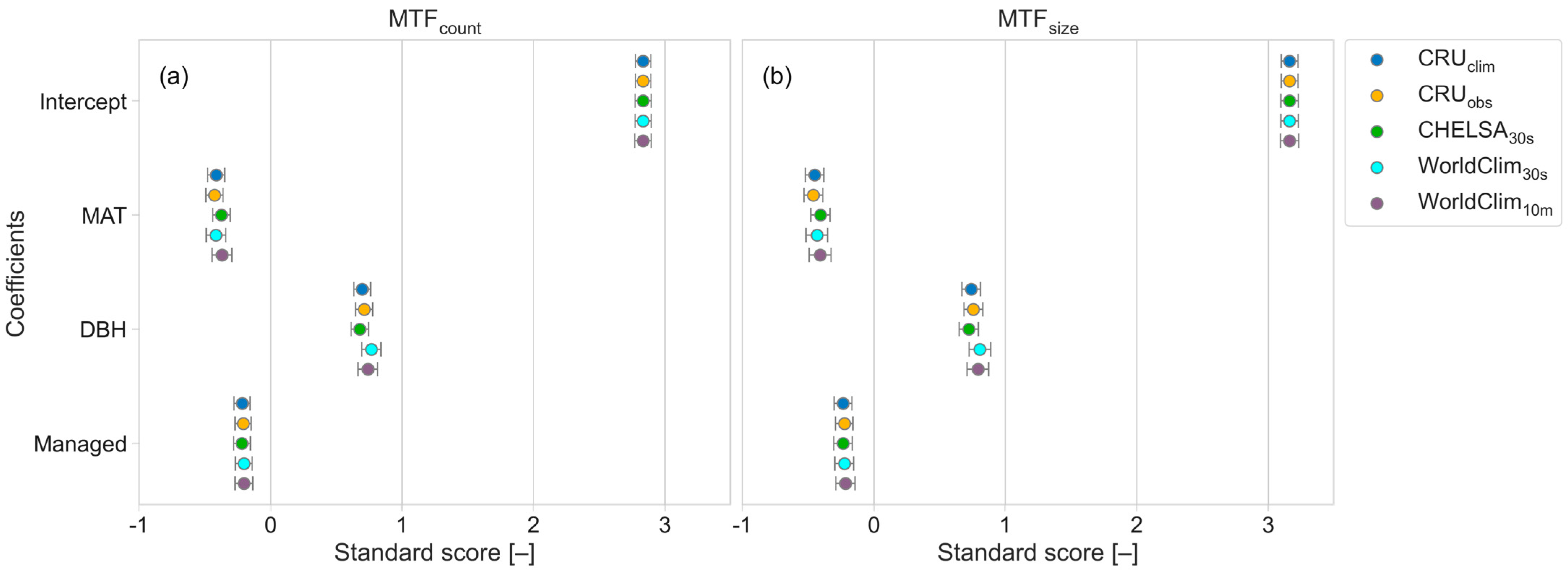
4.3. Climate Influence on the MTF

MAT accelerated DST fall, and MAT was the most important explanatory factor of the MTF for DSTs that died by other causes than fire (Table 4, Figure 6). In the literature, evidence is mixed. Two recent regional studies from Canada and Switzerland did not find a temperature effect on fall rates of DSTs [12], whereas a regional study from the western US also found that DSTs fell faster with increasing temperatures [42]. However, overall, the temperature range analyzed in this study is larger than in any of the cited regional studies, and temperature remained a significant explanatory variable when we tested it for the narrower temperature range of <10 °C, which is consistent with the subset of DSTs that died by fire (Figure 3; Table A2 and Table A5). We therefore find strong evidence for a temperature effect on the MTF of DSTs that died by other causes than fire. It is important to note, however, that at the species level, the MAT was only a significant covariate in combination with tree size (DBH).

As expected by our hypothesis, MAT over the observation period of the MTF (CRU_obs, Figure A1; Table A3) was generally a better explanatory variable than MAT from datasets of two different standardized reference periods (1981–2010 and 1970–2000) and different resolutions (Table A1; Figure A7), as well as soil temperature (MAT_soil; Table A3 and Table A4). Differences between CRU_clim and CRU_obs were marginal, with up to 2% additional explained variation when compared directly for M_All. CRU_obs explained up to 6% more variation than other climate datasets (Table A3). When we distinguished by mortality cause, CRU_obs reliably explained the largest variance in the data (Table A4). CRU_obs possibly performed better than MAT from climate reference periods because survey durations generally only covered a fraction of these standardized reference periods (cf. Figure A1). It is important to note that MAT_soil often explained similar variations in the data compared to CRU but consistently showed a higher RMSE (Table A3), and it was therefore not selected for the final models in Table 4. The high agreement between air and soil temperature has been explained by a generally linear correlation between these variables and the fact that the largest differences in MAT in the air and soil occur at higher latitudes due to snow cover, which insulates the soil from sub-zero temperatures [123]. However, since decomposition is slow at low temperatures, the differences between air and soil temperatures might not be substantial enough to affect DST fall. Wang et al. [141] measured the temperature of woody debris and found that the linear correlation between wood and air temperature broke down only in later decay stages, which are generally not reached for DSTs [7,42,49,77,142].

In this study, using large-scale gridded climate data, we did not detect any influence of moisture availability on the MTF. Of the regional scale DST fall studies [7,42,49,142], only one study explicitly analyzed precipitation as a driver of fall rates, but it did not find an effect [7]. The influence of moisture availability on the MTF in our dataset is not well resolved. Bradford et al. [139] found that soil moisture and wood moisture of wood samples were significant predictors of woody decomposition in DSTs and influenced fall rates. Importantly, wood moisture differed less between the two sites, but was mainly driven by the position of the wood relative to the soil. The variability of decomposition rates within plots has been shown by many studies [8,24] and is likely caused by soil moisture variability, which shows a much higher variation than does temperature at fine scales [24,143], making mean moisture availability from large-scale climate products such as precipitation a weak predictor of woody decomposition [24].

4.4. Substrate Quality Influence on the MTF

Larger tree sizes (DBHs) increased MTFs and, consistent with our expectation, was one of the most important explanatory variables, and was included in all selected species-level regression models independent of mortality group (Table 4 and Table 5; Figure 5 and Figure 6). DSTs standing longer with increasing tree size has been widely reported for local study sites and regions [33,42,74,78,94] and has been connected to lower surface-to-volume ratios, higher amounts of decay-resistant heart wood and higher resistance to breaking forces [15,36], but some studies also found no significant effect or found positive effects of tree size on fall rates [7,10,55]. Our dataset included studies reporting negative, positive and zero effect of tree size [10,55] leading us to conclude that the overall size effect on the MTF is robust when studies are considered together.

For DSTs killed by fire, tree size was the only explanatory factor, and was four times more important for explaining MTFs than for DSTs killed by other causes (M_Other and M_NoFire; Figure 6). It is important to note that the largest tree sizes in this dataset were reported for fire-killed DSTs, wherein the maximum tree size was almost twice as large as for DSTs killed by other causes (Table A2). However, Figure 7 reveals that, all other factors being equal, the MTF response of DSTs killed by fire and mortality by other causes diverge markedly from a DBH of 25 cm, which might suggest that mechanical strength to resist breaking forces is more important than factors driving decomposition for DSTs killed by fire. This interpretation is supported by abundant evidence that fire changes wood properties through heating and charring, which results in generally adverse effects on woody decomposition [144,145,146]. The heating-induced chemical changes of wood have been shown to lower moisture retention capacity [145,147], change wood chemical composition [144,145,148,149,150] and lower nitrogen availability for decomposers [47,147,151]]. In response to these changes, fungi showed lower colonization rates and growth on affected wood, and the negative effects on fungal growth and wood decay generally increased with fire intensity as well as the duration of heating [144,145,148,152,153]. However, the effect on decomposition rates depended on the species of fungi and trees and could range from no effect to substantially lower decomposition rates [152,153,154]. Importantly, increasing fire intensity has also been directly connected to both lower DST fall rates and decomposition rates in DST [75,91,155].

We found statistically significant differences between coniferous and broadleaved plant functional types and mortality causes at the species, but not at the site, level. Although our tests did not control for unbalanced sampling in the dataset, the differences in our regression models, which control for differences in MAT, support the robustness of the effects of fire, tree size and coniferous vs. broadleaved classification.

At the site level, no mortality group indicated plant functional type as a significant covariate. This is likely due to 90%–100% of sites being dominated by coniferous trees across mortality groups (Table A2). Our representation of the PFT at the site level was restricted to PFT dominance due to limited reported information about species composition when authors reported mean site MTFs (Section 2.1.1); therefore, it is possible that a more detailed representation of broadleaved DSTs could have revealed an effect. At the species level, however, the mortality groups M_NoFire and M_Other included plant functional type as a significant covariate, and PFT explained 9% of additional variation for these data groups. In these datasets, the share of coniferous species was 62%–78% (M_NoFire, M_Other; Table A2). Conversely, whereas M_Fire did not include PFT as a covariate, the dataset only included 2% of broadleaved species, making the relationships found for DSTs that died by fire only applicable to coniferous trees.

Coniferous species had higher MTF values than broadleaved species (Figure 4), although there is evidence that broadleaved species can have high decay resistance [40,41,49]. We tested decay resistance as a predictor of MTF for mortality caused by other causes than fire and insects at the species level (n = 60, Table A6) using a published dataset of wood durability, which we expanded using the same methodology (Section 2.1.2; [42]). Wood durability was not a significant covariate for any model; instead, PFT remained the most significant explanatory driver of substrate quality in this direct comparison, further supporting using the distinction into PFTs to explain MTFs (Table 4).

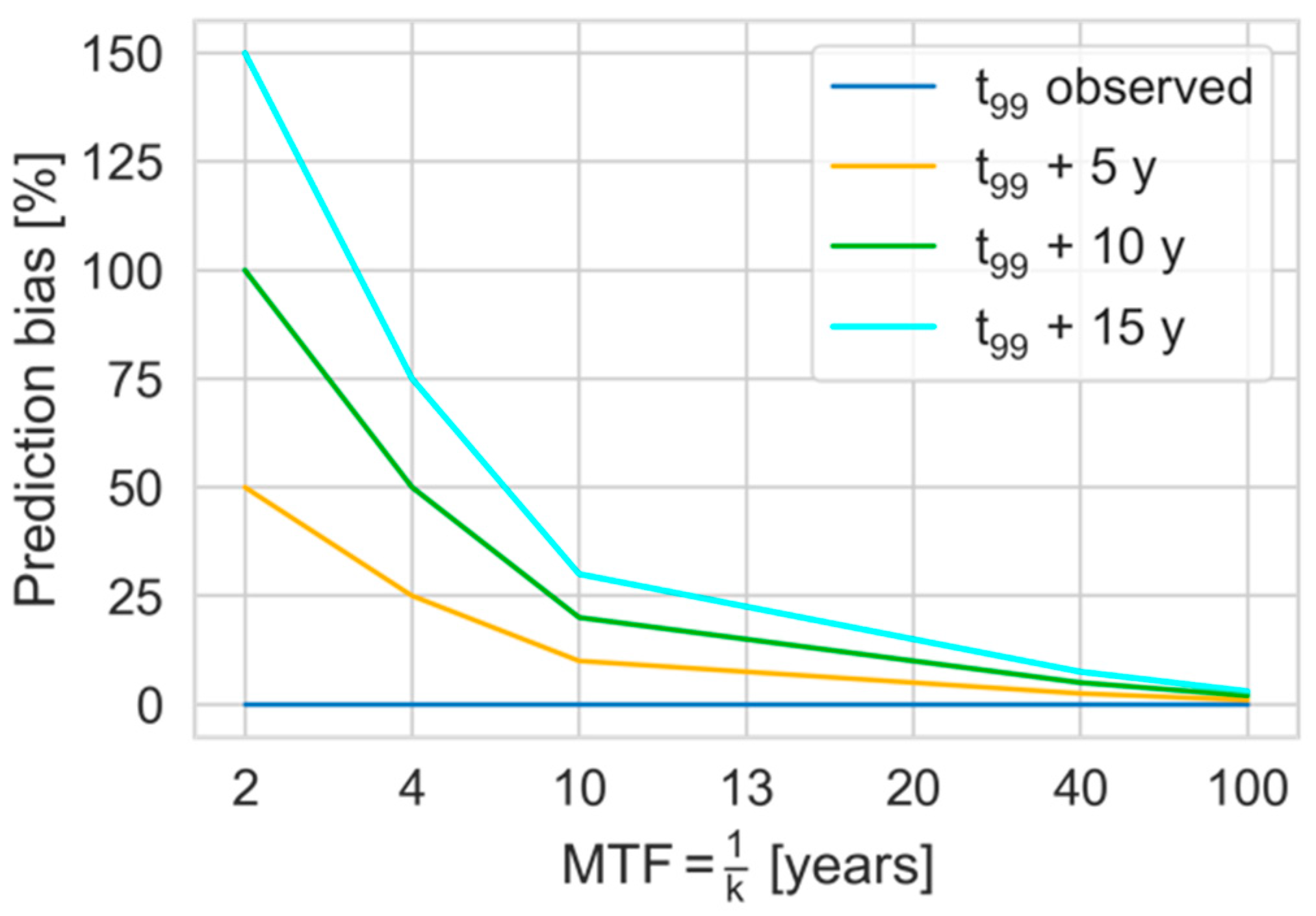
4.5. Analysis Limitations and Outlook

Our study was limited by a lack of reporting of data of DST fall that could be converted to the MTF for all continents except North America. As a result, the best applicability of the regression equations is for the areas of the northern hemisphere which are covered by the range of reported covariates (Table A2). We were able to estimate the MTF across our two tropical sites; however, further data is necessary to support these relationships. Our study was further limited by unstandardized reporting of DST fall data, a low number of observations of trees that died by fire from broadleaf-dominated sites, and short observation periods, which required that we make a range of assumptions. These assumptions might have influenced the estimated MTFs between 1 and 25% across the range reported here (see Equations (4) and (5)), in addition to errors from the original investigations. These uncertainties probably also contributed to high RMSEs, which could be reduced in future DST fall studies with longer observation periods and the reporting of variables that have explained much variation in DST fall in other studies, such as stand density [42,84]. Future studies could also benefit from consistent reporting of DST DBH resolved at the species level, which we suggest should always be part of DST fall studies when feasible.

5. Conclusions

We conducted the first large-scale re-analysis of dead standing tree (DST) fall data, which we express as the mean time to fall (MTF) based on DST counts (MTF_count) and DST counts weighted by the carbon mass at time of death (MTF_size). We presented regression models for different mortality groups, wherein species-level regressions described more variation than site-level regressions. The multiple linear regressions described the MTF as a function of variables important for mechanical resistance to breaking forces and decomposition, i.e., tree size (DBH) and mean annual temperature (MAT). Additional variation was explained by plant functional type and management, though we were unable to test this definitively due to low data availability of broadleaved DST fall and difficulty controlling for potential confounding factors not included here. Further investigation would be valuable to help identify the magnitude of any management effect, and more studies on DST fall of broadleaved trees are needed. The database on DST fall is relatively small in a global context, and a large-scale understanding of DST fall would benefit from data outside North America, especially from the tropics.

References

1. Pan, Y.; Birdsey, R.A.; Fang, J.; Houghton, R.; Kauppi, P.E.; Kurz, W.A.; Phillips, O.L.; Shvidenko, A.; Lewis, S.L.; Canadell, J.G.; et al. A Large and Persistent Carbon Sink in the World’s Forests. Science 2011, 333, 988–993. [Google Scholar] [CrossRef] [PubMed] [Green Version]
2. Pugh, T.A.M.; Arneth, A.; Kautz, M.; Poulter, B.; Smith, B. Important Role of Forest Disturbances in the Global Biomass Turnover and Carbon Sinks. Nat. Geosci. 2019, 12, 730–735. [Google Scholar] [CrossRef] [PubMed]
3. Hubau, W.; Lewis, S.L.; Phillips, O.L.; Affum-Baffoe, K.; Beeckman, H.; Cuní-Sanchez, A.; Daniels, A.K.; Ewango, C.E.N.; Fauset, S.; Mukinzi, J.M.; et al. Asynchronous Carbon Sink Saturation in African and Amazonian Tropical Forests. Nature 2020, 579, 80–87. [Google Scholar] [CrossRef] [PubMed] [Green Version]
4. Tagesson, T.; Schurgers, G.; Horion, S.; Ciais, P.; Tian, F.; Brandt, M.; Ahlström, A.; Wigneron, J.P.; Ardö, J.; Olin, S.; et al. Recent Divergence in the Contributions of Tropical and Boreal Forests to the Terrestrial Carbon Sink. Nat. Ecol. Evol. 2020, 4, 202–209. [Google Scholar] [CrossRef]
5. Seidl, R.; Thom, D.; Kautz, M.; Martin-Benito, D.; Peltoniemi, M.; Vacchiano, G.; Wild, J.; Ascoli, D.; Petr, M.; Honkaniemi, J.; et al. Forest Disturbances under Climate Change. Nat. Clim. Chang. 2017, 7, 395–402. [Google Scholar] [CrossRef] [Green Version]
6. Mackensen, J.; Bauhus, J.; Webber, E. Decomposition Rates of Coarse Woody Debris - A Review with Particular Emphasis on Australian Tree Species. Aust J Bot 2003, 51, 27–37. [Google Scholar] [CrossRef]
7. Hararuk, O.; Kurz, W.A.; Didion, M. Dynamics of Dead Wood Decay in Swiss Forests. For. Ecosyst. 2020, 7, 36. [Google Scholar] [CrossRef]
8. Harmon, M.E.; Fasth, B.G.; Yatskov, M.; Kastendick, D.; Rock, J.; Woodall, C.W. Release of Coarse Woody Detritus-Related Carbon: A Synthesis across Forest Biomes. Carbon Balance Manag. 2020, 15, 1. [Google Scholar] [CrossRef]
9. Yatskov, M.; Harmon, M.E.; Krankina, O.N. A Chronosequence of Wood Decomposition in the Boreal Forests of Russia. Can. J. For. Res. 2003, 33, 1211–1226. [Google Scholar] [CrossRef]
10. Vanderwel, M.C.; Malcolm, J.R.; Smith, S.M. An Integrated Model for Snag and Downed Woody Debris Decay Class Transitions. Ecol. Manag. 2006, 234, 48–59. [Google Scholar] [CrossRef]
11. Mukhortova, L.V.; Kirdianov, A.V.; Myglan, V.S.; Guggenberger, G. Wood Transformation in Dead-Standing Trees in the Forest-Tundra of Central Siberia. Biol. Bull. 2009, 36, 70–78. [Google Scholar] [CrossRef]
12. Hararuk, O.; Shaw, C.; Kurz, W.A. Constraining the Organic Matter Decay Parameters in the CBM-CFS3 Using Canadian National Forest Inventory Data and a Bayesian Inversion Technique. Ecol. Model. 2017, 364, 1–12. [Google Scholar] [CrossRef]
13. Song, Z.; Dunn, C.; Lü, X.-T.T.; Qiao, L.; Pang, J.-P.P.; Tang, J.-W.W. Coarse Woody Decay Rates Vary by Physical Position in Tropical Seasonal Rainforests of SW China. Ecol. Manag. 2017, 385, 206–213. [Google Scholar] [CrossRef] [Green Version]
14. Gora, E.M.; Lucas, J.M.; Yanoviak, S.P. Microbial Composition and Wood Decomposition Rates Vary with Microclimate From the Ground to the Canopy in a Tropical Forest. Ecosystems 2019, 22, 1206–1219. [Google Scholar] [CrossRef]
15. Oberle, B.; Covey, K.R.; Dunham, K.M.; Hernandez, E.J.; Walton, M.L.; Young, D.F.; Zanne, A.E. Dissecting the Effects of Diameter on Wood Decay Emphasizes the Importance of Cross-Stem Conductivity in Fraxinus Americana. Ecosystems 2018, 21, 85–97. [Google Scholar] [CrossRef]
16. Woodall, C.W.; Domke, G.M.; MacFarlane, D.W.; Oswalt, C.M. Comparing Field-and Model-Based Standing Dead Tree Carbon Stock Estimates across Forests of the US. Forestry 2012, 85, 125–133. [Google Scholar] [CrossRef] [Green Version]
17. Aakala, T.; Kuuluvainen, T.; Gauthier, S.; De Grandpré, L. Standing Dead Trees and Their Decay-Class Dynamics in the Northeastern Boreal Old-Growth Forests of Quebec. Ecol. Manag. 2008, 255, 410–420. [Google Scholar] [CrossRef]
18. Linder, P. Structural Changes in Two Virgin Boreal Forest Stands in Central Sweden over 72 Years. Scand. J. For. Res. 1998, 13, 451–461. [Google Scholar] [CrossRef]
19. Josefsson, T.; Gunnarson, B.; Liedgren, L.; Bergman, I.; Östlund, L. Historical Human Influence on Forest Composition and Structure in Boreal Fennoscandia. Can. J. For. Res. 2010, 40, 872–884. [Google Scholar] [CrossRef]
20. Cook, G.D.; Liedloff, A.C.; Meyer, C.P.M.; Richards, A.E.; Bray, S.G. Standing Dead Trees Contribute Significantly to Carbon Budgets in Australian Savannas. Int. J. Wildland Fire 2020, 29, 215–228. [Google Scholar] [CrossRef]
21. Delaney, M.; Brown, S.; Lugo, A.E.; Torres-Lezama, A.; Quintero, N.B. The Quantity and Turnover of Dead Wood in Permanent Forest Plots in Six Life Zones of Venezuela 1. Biotropica 1998, 30, 2–11. [Google Scholar] [CrossRef]
22. Gora, E.M.; Kneale, R.C.; Larjavaara, M.; Muller-Landau, H.C. Dead Wood Necromass in a Moist Tropical Forest: Stocks, Fluxes, and Spatiotemporal Variability. Ecosystems 2019, 22, 1189–1205. [Google Scholar] [CrossRef]
23. Harmon, M.E.; Krankina, O.N.; Sexton, J. Decomposition Vectors: A New Approach to Estimating Woody Detritus Decomposition Dynamics. Can. J. For. Res. 2000, 30, 76–84. [Google Scholar] [CrossRef]
24. Bradford, M.A.; Warren, R.J.; Baldrian, P.; Crowther, T.W.; Maynard, D.S.; Oldfield, E.E.; Wieder, W.R.; Wood, S.A.; King, J.R. Climate Fails to Predict Wood Decomposition at Regional Scales. Nat. Clim. Chang. 2014, 4, 625–630. [Google Scholar] [CrossRef] [Green Version]
25. Krankina, O.N.; Harmon, M.E. Dynamics of the Dead Wood Carbon Pool in Northwestern Russian Boreal Forests. Water Air Soil Pollut. 1995, 82, 227–238. [Google Scholar] [CrossRef]
26. Storaunet, K.O.; Rolstad, J. Time since Death and Fall of Norway Spruce Logs in Old-Growth and Selectively Cut Boreal Forest. Can. J. For. Res. 2002, 32, 1801–1812. [Google Scholar] [CrossRef]
27. Boulanger, Y.; Sirois, L. Postfire Dynamics of Black Spruce Coarse Woody Debris in Northern Boreal Forest of Quebec. Can. J. For. Res. 2006, 36, 1770–1780. [Google Scholar] [CrossRef] [Green Version]
28. Angers, V.A.; Drapeau, P.; Bergeron, Y. Snag Degradation Pathways of Four North American Boreal Tree Species. Ecol. Manag. 2010, 259, 246–256. [Google Scholar] [CrossRef]
29. Friedlingstein, P.; Jones, M.W.; O’Sullivan, M.; Andrew, R.M.; Bakker, D.C.E.; Hauck, J.; Le Quéré, C.; Peters, G.P.; Peters, W.; Pongratz, J.; et al. Global Carbon Budget 2021. Earth Syst. Sci. Data 2022, 14, 1917–2005. [Google Scholar] [CrossRef]
30. Brienen, R.J.W.; Phillips, O.L.; Feldpausch, T.R.; Gloor, E.; Baker, T.R.; Lloyd, J.; Lopez-Gonzalez, G.; Monteagudo-Mendoza, A.; Malhi, Y.; Lewis, S.L.; et al. Long-Term Decline of the Amazon Carbon Sink. Nature 2015, 519, 344–348. [Google Scholar] [CrossRef] [PubMed] [Green Version]
31. van Mantgem, P.J.; Stephenson, N.L.; Byrne, J.C.; Daniels, L.D.; Franklin, J.F.; Fulé, P.Z.; Harmon, M.E.; Larson, A.J.; Smith, J.M.; Taylor, A.H.; et al. Widespread Increase of Tree Mortality Rates in the Western United States. Science 2009, 323, 521–524. [Google Scholar] [CrossRef] [PubMed] [Green Version]
32. Peltola, H.M. Mechanical Stability of Trees under Static Loads. Am. J. Bot. 2006, 93, 1501–1511. [Google Scholar] [CrossRef] [PubMed]
33. Harmon, M.E.; Franklin, J.F.; Swanson, F.J.; Sollins, P.; Gregory, S.V.; Lattin, J.D.; Anderson, N.H.; Cline, S.P.; Aumen, N.G.; Sedell, J.R.; et al. Ecology of Coarse Woody Debris in Temperate Ecosystems. Adv. Ecol. Res. 1986, 15, 135–305. [Google Scholar] [CrossRef]
34. Zanne, A.E.; Oberle, B.; Dunham, K.M.; Milo, A.M.; Walton, M.L.; Young, D.F. A Deteriorating State of Affairs: How Endogenous and Exogenous Factors Determine Plant Decay Rates. J. Ecol. 2015, 103, 1421–1431. [Google Scholar] [CrossRef] [Green Version]
35. Hu, Z.; Michaletz, S.T.; Johnson, D.J.; McDowell, N.G.; Huang, Z.; Zhou, X.; Xu, C. Traits Drive Global Wood Decomposition Rates More than Climate. Glob. Chang. Biol. 2018, 24, 5259–5269. [Google Scholar] [CrossRef]
36. Tuomi, M.; Laiho, R.; Repo, A.; Liski, J. Wood Decomposition Model for Boreal Forests. Ecol. Model. 2011, 222, 709–718. [Google Scholar] [CrossRef]
37. Weedon, J.T.; Cornwell, W.K.; Cornelissen, J.H.C.C.; Zanne, A.E.; Wirth, C.; Coomes, D.A. Global Meta-Analysis of Wood Decomposition Rates: A Role for Trait Variation among Tree Species? Ecol. Lett. 2009, 12, 45–56. [Google Scholar] [CrossRef]
38. Kahl, T.; Baber, K.; Otto, P.; Wirth, C.; Bauhus, J. Drivers of CO2 Emission Rates from Dead Wood Logs of 13 Tree Species in the Initial Decomposition Phase. Forests 2015, 6, 2484–2504. [Google Scholar] [CrossRef] [Green Version]
39. Kipping, L.; Gossner, M.M.; Koschorreck, M.; Muszynski, S.; Maurer, F.; Weisser, W.W.; Jehmlich, N.; Noll, M. Emission of CO2 and CH4 From 13 Deadwood Tree Species Is Linked to Tree Species Identity and Management Intensity in Forest and Grassland Habitats. Glob. Biogeochem. Cycles 2022, 36, e2021GB007143. [Google Scholar] [CrossRef]
40. Scheffer, T.C.; Cowling, E.B. Natural Resistance of Wood to Microbial Deterioration. Annu. Rev. Phytopathol. 1966, 4, 147–168. [Google Scholar] [CrossRef]
41. Scheffer, T.C.; Morrell, J.J. Natural Durability of Wood: A Worldwide Checklist of Species; Research Contribution 22; Forest Research Laboratory, Oregon State University: Corvallis, OR, USA, 1998. [Google Scholar]
42. Oberle, B.; Ogle, K.; Zanne, A.E.; Woodall, C.W. When a Tree Falls: Controls on Wood Decay Predict Standing Dead Tree Fall and New Risks in Changing Forests. PLoS ONE 2018, 13, e0196712. [Google Scholar] [CrossRef] [PubMed] [Green Version]
43. Josefsson, T.; Olsson, J.; Östlund, L. Linking Forest History and Conservation Efforts: Long-Term Impact of Low-Intensity Timber Harvest on Forest Structure and Wood-Inhabiting Fungi in Northern Sweden. Biol. Conserv. 2010, 143, 1803–1811. [Google Scholar] [CrossRef]
44. Pastorelli, R.; Paletto, A.; Agnelli, A.E.; Lagomarsino, A.; De Meo, I. Microbial Diversity and Ecosystem Functioning in Deadwood of Black Pine of a Temperate Forest. Forests 2021, 12, 1418. [Google Scholar] [CrossRef]
45. Mitchell, R.G.; Preisler, H.K. Fall Rate of Lodgepole Pine Killed by the Mountain Pine Beetle in Central Oregon. West. J. Appl. For. 1998, 13, 23–26. [Google Scholar] [CrossRef] [Green Version]
46. Wei, X.; Kimmins, J.P. Asymbiotic Nitrogen Fixation in Harvested and Wildfire-Killed Lodgepole Pine Forests in the Central Interior of British Columbia. Ecol. Manag. 1998, 109, 343–353. [Google Scholar] [CrossRef]
47. Hanula, J.L.; Ulyshen, M.D.; Wade, D.D. Impacts of Prescribed Fire Frequency on Coarse Woody Debris Volume, Decomposition and Termite Activity in the Longleaf Pine Flatwoods of Florida. Forests 2012, 3, 317–331. [Google Scholar] [CrossRef]
48. Schroeder, L.M. Retention or Salvage Logging of Standing Trees Killed by the Spruce Bark Beetle Ips Typographus: Consequences for Dead Wood Dynamics and Biodiversity. Scand. J. For. Res. 2007, 22, 524–530. [Google Scholar] [CrossRef]
49. Hilger, A.B.; Shaw, C.H.; Metsaranta, J.M.; Kurz, W.A. Estimation of Snag Carbon Transfer Rates by Ecozone and Lead Species for Forests in Canada. Ecol. Appl. 2012, 22, 2078–2090. [Google Scholar] [CrossRef]
50. Smith, C.Y.; Moroni, M.T.; Warkentin, I.G. Snag Dynamics in Post-Harvest Landscapes of Western Newfoundland Balsam Fir-Dominated Boreal Forests. Ecol. Manag. 2009, 258, 832–839. [Google Scholar] [CrossRef]
51. Cline, S.P.; Berg, A.B.; Wight, H.M. Snag Characteristics and Dynamics in Douglas-Fir Forests, Western Oregon. J. Wildl. Manag. 1980, 44, 773. [Google Scholar] [CrossRef]
52. Everett, R.; Lehmkuhl, J.; Schellhaas, R.; Ohlson, P.; Keenum, D.; Riesterer, H.; Spurbeck, D. Snag Dynamics in a Chronosequence of 26 Wildfires on the East Slope of the Cascade Range in Washington State, USA. Int. J. Wildland Fire 1999, 9, 223–234. [Google Scholar] [CrossRef]
53. Huggard, D.J. Static Life-Table Analysis of Fall Rates of Subalpine Fir Snags. Ecol. Appl. 1999, 9, 1009–1016. [Google Scholar] [CrossRef]
54. Sinclair, R. Persistence of Dead Trees and Fallen Timber in the Arid Zone: 76 Years of Data from the T.G.B. Osborn Vegetation Reserve, Koonamore, South Australia. Rangel. J. 2004, 26, 111–122. [Google Scholar] [CrossRef]
55. Mäkinen, H.; Hynynen, J.; Siitonen, J.; Sievänen, R. Predicting the Decomposition of Scots Pine, Norway Spruce, and Birch Stems in Finland. Ecol. Appl. 2006, 16, 1865–1879. [Google Scholar] [CrossRef] [PubMed]
56. Bond-Lamberty, B.; Gower, S.T. Decomposition and Fragmentation of Coarse Woody Debris: Re-Visiting a Boreal Black Spruce Chronosequence. Ecosystems 2008, 11, 831–840. [Google Scholar] [CrossRef]
57. Metsaranta, J.M.; Lieffers, V.J.; Wein, R.W. Dendrochronological Reconstruction of Jack Pine Snag and Downed Log Dynamics in Saskatchewan and Manitoba, Canada. Ecol. Manag. 2008, 255, 1262–1270. [Google Scholar] [CrossRef]
58. DeLong, S.C.; Sutherland, G.D.; Daniels, L.D.; Heemskerk, B.H.; Storaunet, K.O. Temporal Dynamics of Snags and Development of Snag Habitats in Wet Spruce-Fir Stands in East-Central British Columbia. Ecol. Manag. 2008, 255, 3613–3620. [Google Scholar] [CrossRef]
59. Lyon, L.J. Attrition of Lodgepole Pine Snags on the Sleeping Child Burn, Montana; Department of Agriculture, Forest Service, Intermountain Forest and Range Experiment Station: Ogden, UT, USA, 1977; Volume 219.
60. Yamasaki, M.; Leak, W.B. Snag Longevity in Managed Northern Hardwoods. North. J. Appl. For. 2006, 23, 215–217. [Google Scholar] [CrossRef] [Green Version]
61. Onodera, K.; Tokuda, S. Do Larger Snags Stand Longer?—Snag Longevity in Mixed Conifer–Hardwood Forests in Hokkaido, Japan. Ann. Sci. 2015, 72, 621–629. [Google Scholar] [CrossRef] [Green Version]
62. Slaughter, K.W.; Grigal, D.F.; Ohmann, L.F. Carbon Storage in Southern Boreal Forests Following Fire. Scand. J. For. Res. 1998, 13, 119–127. [Google Scholar] [CrossRef]
63. Parish, R.; Antos, J.A.; Ott, P.K.; Lucca, C.M. Di Snag Longevity of Douglas-Fir, Western Hemlock, and Western Redcedar from Permanent Sample Plots in Coastal British Columbia. Ecol. Manag. 2010, 259, 633–640. [Google Scholar] [CrossRef]
64. Raphael, M.; Morrison, M. Decay and Dynamics of Snags in the Sierra Nevada, California. For. Sci. 1987, 33, 774–783. [Google Scholar]
65. Bull, E.B. Longevity of Snags and Their Use by Woodpeckers. In Snag Habitat Management: Proceedings of the Symposium, USDA Forestry Service General Technical Report RM-99; Coordinators, T., Davis, J., Goodwin, G., Ockenfels, R., Eds.; U.S. Department of Agriculture, Forest Service, Rocky Mountain Research Station: Fort Collins, CO, USA, 1983; pp. 64–67. [Google Scholar]
66. Kearns, H.S.J.; Jacobi, W.R.; Johnson, D.W. Persistence of Pinyon Pine Snags and Logs in Southwestern Colorado. West. J. Appl. For. 2005, 20, 247–252. [Google Scholar] [CrossRef] [Green Version]
67. Harrington, M.G. Fall Rates of Prescribed Fire-Killed Ponderosa Pine; United States Department of Agriculture-Forest Service: Washington, DC, USA, 1996.
68. Woolley, T.; Shaw, D.C.; Hollingsworth, L.W.T.; Agne, M.C.; Fitzgerald, S.; Eglitis, A.; Kurth, L. Beyond Red Crowns: Complex Changes in Surface and Crown Fuels and Their Interactions 32 Years Following Mountain Pine Beetle Epidemics in South-Central Oregon, USA. Fire Ecol. 2019, 15, 4. [Google Scholar] [CrossRef]
69. Garber, S.M.; Brown, J.P.; Wilson, D.S.; Maguire, D.A.; Heath, L.S. Snag Longevity under Alternative Silvicultural Regimes in Mixed-Species Forests of Central Maine. Can. J. For. Res. 2005, 35, 787–796. [Google Scholar] [CrossRef]
70. Moorman, C.E.; Russell, K.R.; Sabin, G.R.; Guynn, D.C., Jr. Snag Dynamics and Cavity Occurrence in the South Carolina Piedmont. Ecol. Manag. 1999, 118, 37–48. [Google Scholar] [CrossRef]
71. Wilson, B.F.; McComb, B.C. Dynamics of Dead Wood over 20 Years in a New England Oak Forest. Can. J. For. Res. 2005, 35, 682–692. [Google Scholar] [CrossRef]
72. Taylor, S.L.; MacLean, D.A. Dead Wood Dynamics in Declining Balsam Fir and Spruce Stands in New Brunswick, Canada. Can. J. For. Res. 2007, 37, 750–762. [Google Scholar] [CrossRef]
73. Conner, R.N.; Saenz, D. The Longevity of Large Pine Snags in Eastern Texas. Wildl. Soc. Bull. 2005, 33, 700–705. [Google Scholar] [CrossRef]
74. Dunn, C.J.; Bailey, J.D. Temporal Dynamics and Decay of Coarse Wood in Early Seral Habitats of Dry-Mixed Conifer Forests in Oregon’s Eastern Cascades. Ecol. Manag. 2012, 276, 71–81. [Google Scholar] [CrossRef]
75. Dunn, C.J.; Bailey, J.D. Temporal Fuel Dynamics Following High-Severity Fire in Dry Mixed Conifer Forests of the Eastern Cascades, Oregon, USA. Int. J. Wildland Fire 2015, 24, 470–483. [Google Scholar] [CrossRef]
76. Hart, J.H.; Hart, D.L. Heartrot Fungi’s Role in Creating Picid Nesting Sites in Living Aspen. In Sustaining Aspen in Western Landscapes: Symposium; U.S. Department of Agriculture, Forest Service, Rocky Mountain Research Station: Fort Collins, CO, USA, 2001; pp. 207–213. [Google Scholar]
77. Holeksa, J.; Zielonka, T.; Zywiec, M. Modeling the Decay of Coarse Woody Debris in a Subalpine Norway Spruce Forest of the West Carpathians, Poland. Can. J. For. Res. 2008, 38, 415–428. [Google Scholar] [CrossRef]
78. Dunn, C.J.; Bailey, J.D. Tree Mortality and Structural Change Following Mixed-Severity Fire in Pseudotsuga Forests of Oregon’s Western Cascades, USA. Ecol. Manag. 2016, 365, 107–118. [Google Scholar] [CrossRef]
79. Landram, F.M.; Laudenslayer, W.F.; Atzet, T. Demography of Snags in Eastside Pine Forests of California. In General Technical Report PSW-GTR-181, Proceedings of the Symposium on the Ecology and Management of Dead Wood in Western Forests, Reno, NV, USA, 2–4 November 1999; U.S. Department of Agriculture, Forest Service, Pacific Southwest Research Station: Albany, CA, USA, 2002. [Google Scholar]
80. Siccama, T.G.; Fahey, T.J.; Johnson, C.E.; Sherry, T.W.; Denny, E.G.; Girdler, E.B.; Likens, G.E.; Schwarz, P.A. Population and Biomass Dynamics of Trees in a Northern Hardwood Forest at Hubbard Brook. Can. J. For. Res. 2007, 37, 737–749. [Google Scholar] [CrossRef]
81. Brown, M.J.; Kertis, J.; Huff, M.H. Natural Tree Regeneration and Coarse Woody Debris Dynamics after a Forest Fire in the Western Cascade Range; United States Department of Agriculture, Forest Service, Pacific Northwest Research Station: Portland, OR, USA, 2013; Volume 592, pp. 1–50. [CrossRef] [Green Version]
82. Chambers, C.L.; Mast, J.N. Snag Dynamics and Cavity Excavation after Bark Beetle Outbreaks in Southwestern Ponderosa Pine Forests. For. Sci. 2014, 60, 713–723. [Google Scholar] [CrossRef]
83. Stevens-Rumann, C.S.; Hudak, A.T.; Morgan, P.; Arnold, A.; Strand, E.K. Fuel Dynamics Following Wildfire in US Northern Rockies Forests. Front. For. Glob. Chang. 2020, 3, 51. [Google Scholar] [CrossRef]
84. Russell, R.E.; Saab, V.A.; Dudley, J.G.; Rotella, J.J. Snag Longevity in Relation to Wildfire and Postfire Salvage Logging. Ecol. Manag. 2006, 232, 179–187. [Google Scholar] [CrossRef]
85. Dobbertin, M.; Baltensweiler, A.; Rigling, D. Tree Mortality in an Unmanaged Mountain Pine (Pinus Mugo Var. Uncinata) Stand in the Swiss National Park Impacted by Root Rot Fungi. Ecol. Manag. 2001, 145, 79–89. [Google Scholar] [CrossRef]
86. Acker, S.A.; Kertis, J.; Bruner, H.; O’Connell, K.; Sexton, J. Dynamics of Coarse Woody Debris Following Wildfire in a Mountain Hemlock (Tsuga Mertensiana) Forest. Ecol. Manag. 2013, 302, 231–239. [Google Scholar] [CrossRef]
87. Zarnoch, S.J.; Vukovich, M.A.; Kilgo, J.C.; Blake, J.I. Snag Characteristics and Dynamics Following Natural and Artificially Induced Mortality in a Managed Loblolly Pine Forest. Can. J. For. Res. 2013, 43, 817–825. [Google Scholar] [CrossRef]
88. Chambers, C.L.; Mast, J.N. Ponderosa Pine Snag Dynamics and Cavity Excavation Following Wildfire in Northern Arizona. Ecol. Manag. 2005, 216, 227–240. [Google Scholar] [CrossRef]
89. Nelson, K.N.; Turner, M.G.; Romme, W.H.; Tinker, D.B. Landscape Variation in Tree Regeneration and Snag Fall Drive Fuel Loads in 24-Year Old Post-Fire Lodgepole Pine Forests. Ecol. Appl. 2016, 26, 2422–2436. [Google Scholar] [CrossRef] [PubMed]
90. Newbery, J.E.; Lewis, K.J.; Walters, M.B. Inonotus Tomentosus and the Dynamics of Unmanaged and Partial-Cut Wet Sub-Boreal Spruce-Fir Forests. Can. J. For. Res. 2007, 37, 2663–2676. [Google Scholar] [CrossRef]
91. Angers, V.A.; Gauthier, S.; Drapeau, P.; Jayen, K.; Bergeron, Y. Tree Mortality and Snag Dynamics in North American Boreal Tree Species after a Wildfire: A Long-Term Study. Int. J. Wildland Fire 2011, 20, 751. [Google Scholar] [CrossRef]
92. Ganey, J.L.; Vojta, S.C. Trends in Snag Populations in Drought-Stressed Mixed-Conifer and Ponderosa Pine Forests (1997–2007). Int. J. For. Res. 2012, 2012, 1–8. [Google Scholar] [CrossRef] [Green Version]
93. Hogg, E.H.; Michaelian, M. Factors Affecting Fall down Rates of Dead Aspen (Populus Tremuloides) Biomass Following Severe Drought in West-Central Canada. Glob. Chang. Biol. 2015, 21, 1968–1979. [Google Scholar] [CrossRef]
94. Grayson, L.M.; Cluck, D.R.; Hood, S.M. Persistence of Fire-Killed Conifer Snags in California, USA. Fire Ecol. 2019, 15, 1–14. [Google Scholar] [CrossRef] [Green Version]
95. Palace, M.; Keller, M.; Silva, H. Necromass Production: Studies in Undisturbed and Logged Amazon Forests. Ecol. Appl. 2008, 18, 873–884. [Google Scholar] [CrossRef] [PubMed]
96. Ritchie, M.W.; Knapp, E.E. Establishment of a Long-Term Fire Salvage Study in an Interior Ponderosa Pine Forest. J. For. 2014, 112, 395–400. [Google Scholar] [CrossRef]
97. Campbell, J.L.; Fontaine, J.B.; Donato, D.C. Carbon Emissions from Decomposition of Fire-Killed Trees Following a Large Wildfire in Oregon, United States. J. Geophys. Res. Biogeosci. 2016, 121, 718–730. [Google Scholar] [CrossRef]
98. Fassnacht, K.S.; Steele, T.W. Snag Dynamics in Northern Hardwood Forests under Different Management Scenarios. Ecol. Manag. 2016, 363, 267–276. [Google Scholar] [CrossRef] [Green Version]
99. Perera, A.H.; Dalziel, B.D.; Buse, L.J.; Routledge, R.G.; Brienesse, M. What Happens to Tree Residuals in Boreal Forest Fires and What Causes the Changes? Forest Research Report No. 174; Ontario Ministry of Natural Resources: Sault Ste. Marie, ON, Canada, 2011; ISBN 0381-3924 978-1-4435-7268-2. [Google Scholar]
100. Rhoades, C.C.; Hubbard, R.M.; Hood, P.R.; Starr, B.J.; Tinker, D.B.; Elder, K. Snagfall the First Decade after Severe Bark Beetle Infestation of High-Elevation Forests in Colorado, USA. Ecol. Appl. 2020, 30, e02059. [Google Scholar] [CrossRef] [PubMed]
101. Molinas-González, C.R.; Leverkus, A.B.; Marañón-Jiménez, S.; Castro, J. Fall Rate of Burnt Pines across an Elevational Gradient in a Mediterranean Mountain. Eur. J. Res. 2017, 136, 401–409. [Google Scholar] [CrossRef]
102. Corace, R.G.; Seefelt, N.E.; Goebel, P.C.; Shaw, H.L. Snag Longevity and Decay Class Development in a Recent Jack Pine Clearcut in Michigan. North. J. Appl. For. 2010, 27, 125–131. [Google Scholar] [CrossRef] [Green Version]
103. Aakala, T. Coarse Woody Debris in Late-Successional Picea Abies Forests in Northern Europe: Variability in Quantities and Models of Decay Class Dynamics. Ecol. Manag. 2010, 260, 770–779. [Google Scholar] [CrossRef]
104. Alexeyev, V.A.; Birdsey, R.A. (Eds.) Carbon Storage in Forests and Peatlands of Russia; General Technical Report NE-244; U.S. Department of Agriculture, Forest Service, Northeastern Research Station: Radnor, PA, USA, 1998; 137p.
105. Hagemann, U.; Moroni, M.T.; Shaw, C.H.; Kurz, W.A.; Makeschin, F. Comparing Measured and Modelled Forest Carbon Stocks in High-Boreal Forests of Harvest and Natural-Disturbance Origin in Labrador, Canada. Ecol. Model. 2010, 221, 825–839. [Google Scholar] [CrossRef]
106. Hall, S.A.; Burke, C.; Hobbs, N.T. Litter and Dead Wood Dynamics in Ponderosa Pine Forests along a 160-Year Chronosequence. Ecol. Appl. 2006, 16, 2344–2355. [Google Scholar] [CrossRef]
107. Lee, P. Dynamics of Snags in Aspen-Dominated Midboreal Forests. Ecol. Manag. 1998, 105, 263–272. [Google Scholar] [CrossRef]
108. Mellen, K.; Ager, A. A Coarse Wood Dynamics Model for the Western Cascades. In General Technical Report PSW-GTR-181, Proceedings of the Symposium on the Ecology and Management of Dead Wood in Western Forests, Reno, NV, USA, 2–4 November 1999; U.S. Department of Agriculture, Forest Service, Pacific Southwest Research Station: Albany, CA, USA, 2002; Volume 97801, pp. 503–516. [Google Scholar]
109. Moroni, M.T. Disturbance History Affects Dead Wood Abundance in Newfoundland Boreal Forests. Can. J. For. Res. 2006, 36, 3194–3208. [Google Scholar] [CrossRef]
110. Storaunet, K.O.; Rolstad, J. How Long Do Norway Spruce Snags Stand? Evaluating Four Estimation Methods. Can. J. For. Res. 2004, 34, 376–383. [Google Scholar] [CrossRef]
111. Vanderwel, M.C.; Caspersen, J.P.; Woods, M.E. Snag Dynamics in Partially Harvested and Unmanaged Northern Hardwood Forests. Can. J. For. Res. 2006, 36, 2769–2779. [Google Scholar] [CrossRef] [Green Version]
112. Moher, D.; Liberati, A.; Tetzlaff, J.; Altman, D.G. Preferred Reporting Items for Systematic Reviews and Meta-Analyses: The PRISMA Statement. BMJ 2009, 339, 332–336. [Google Scholar] [CrossRef] [PubMed] [Green Version]
113. Ritchie, M.W.; Knapp, E.E.; Skinner, C.N. Snag Longevity and Surface Fuel Accumulation Following Post-Fire Logging in a Ponderosa Pine Dominated Forest. Ecol. Manag. 2013, 287, 113–122. [Google Scholar] [CrossRef]
114. Lehmkuhl, J.F.; Everett, R.L.; Schellhaas, R.; Ohlson, P.; Keenum, D.; Riesterer, H.; Spurbeck, D. Cavities in Snags along a Wildfire Chronosequence in Eastern Washington. J. Wildl. Manag. 2003, 219–228. [Google Scholar] [CrossRef]
115. Kenefic, L.; Brissette, J.; Russell, M.; Puhlick, J. Overstory Tree and Regeneration Data from the “Silvicultural Effects on Composition, Structure, and Growth”. In Penobscot Experimental Forest, 2nd ed.; Forest Service Research Data Archive; U.S. Department of Agriculture, Forest Service, Rocky Mountain Research Station: Fort Collins, CO, USA, 2015. [Google Scholar]
116. Bull, E.L. Habitat Utilization of the Pileated Woodpecker, Blue Mountains, Oregon. Master’s Thesis, Oregon State University, Corvallis, OR, USA, 1975. [Google Scholar]
117. Viovy, N. CRUNCEP Version 7—Atmospheric Forcing Data for the Community Land Model. Available online: https://rda.ucar.edu/datasets/ds314.3/ (accessed on 27 April 2022).
118. Karger, D.N.; Conrad, O.; Böhner, J.; Kawohl, T.; Kreft, H.; Soria-Auza, R.W.; Zimmermann, N.E.; Linder, H.P.; Kessler, M. Climatologies at High Resolution for the Earth’s Land Surface Areas. Sci. Data 2017, 4, 170122. [Google Scholar] [CrossRef] [PubMed] [Green Version]
119. Karger, D.N.; Conrad, O.; Böhner, J.; Kawohl, T.; Kreft, H.; Soria-Auza, R.W.; Zimmermann, N.E.; Linder, H.P.; Kessler, M. Climatologies at High Resolution for the Earth’s Land Surface Areas [Data Set]. EnviDat. Available online: https://envidat.ch/#/metadata/chelsa-climatologies (accessed on 21 April 2022).
120. Fick, S.E.; Hijmans, R.J. WorldClim 2: New 1-Km Spatial Resolution Climate Surfaces for Global Land Areas. Int. J. Climatol. 2017, 37, 4302–4315. [Google Scholar] [CrossRef]
121. Lembrechts, J.J.; van den Hoogen, J.; Aalto, J.; Ashcroft, M.B.; De Frenne, P.; Kemppinen, J.; Kopecký, M.; Luoto, M.; Maclean, I.M.D.; Crowther, T.W.; et al. Global Maps of Soil Temperature. Glob. Chang. Biol. 2022, 28, 3110–3144. [Google Scholar] [CrossRef] [PubMed]
122. van den Hoogen, J.; Lembrechts, J.; Nijs, I.; Lenoir, J. Global Soil Bioclimatic Variables at 30 Arc Second Resolution Version 1 [Data Set]. Available online: https://zenodo.org/record/4558732#.ZGIJLqVByUk (accessed on 21 April 2022).
123. Guglielmo, M.; Tang, F.H.M.; Pasut, C.; Maggi, F. SOIL-WATERGRIDS, Mapping Dynamic Changes in Soil Moisture and Depth of Water Table from 1970 to 2014. Sci. Data 2021, 8, 263. [Google Scholar] [CrossRef]
124. Maggi, F.; Guglielmo, M.; Tang, F.H.M.M.; Pasut, C. SOIL-WATERGRIDS v1, Mapping Dynamic Changes in Soil Moisture and Depth of Water Table from 1970 to 2014, Dataset and Modelling (Version v1) [Data Set]. Available online: https://zenodo.org/record/4997453#.ZGIJ3qVByUk (accessed on 25 January 2023).
125. Dormann, C.F.; Elith, J.; Bacher, S.; Buchmann, C.; Carl, G.; Carré, G.; Marquéz, J.R.G.; Gruber, B.; Lafourcade, B.; Leitão, P.J.; et al. Collinearity: A Review of Methods to Deal with It and a Simulation Study Evaluating Their Performance. Ecography 2013, 36, 27–46. [Google Scholar] [CrossRef]
126. Kattge, J.; Bönisch, G.; Díaz, S.; Lavorel, S.; Prentice, I.C.; Leadley, P.; Tautenhahn, S.; Werner, G.D.A.; Aakala, T.; Abedi, M.; et al. TRY Plant Trait Database – Enhanced Coverage and Open Access. Glob. Chang. Biol. 2020, 26, 119–188. [Google Scholar] [CrossRef] [Green Version]
127. Olson, J.S. Energy Storage and the Balance of Producers and Decomposers in Ecological Systems. Ecology 1963, 44, 322–331. [Google Scholar] [CrossRef] [Green Version]
128. Rohatgi, A. Webplotdigitizer: Version 4.6 [Computer Software]. Available online: https://automeris.io/WebPlotDigitizer (accessed on 22 September 2021).
129. Virtanen, P.; Gommers, R.; Oliphant, T.E.; Haberland, M.; Reddy, T.; Cournapeau, D.; Burovski, E.; Peterson, P.; Weckesser, W.; Bright, J.; et al. SciPy 1.0: Fundamental Algorithms for Scientific Computing in Python. Nat. Methods 2020, 17, 261–272. [Google Scholar] [CrossRef] [Green Version]
130. Chojnacky, D.C.; Heath, L.S.; Jenkins, J.C. Updated Generalized Biomass Equations for North American Tree Species. Forestry 2014, 87, 129–151. [Google Scholar] [CrossRef] [Green Version]
131. Kershaw, J.A.; Ducey, M.J.; Beers, T.W.; Husch, B. Forest Mensuration; Wiley-Blackwell: Oxford, UK, 2017; ISBN 9781118902035. [Google Scholar]
132. Chambers, J.Q.; Higuchi, N.; Schimel, J.P.; Ferreira, L.V.; Melack, J.M. Decomposition and Carbon Cycling of Dead Trees in Tropical Forests of the Central Amazon. Oecologia 2000, 122, 380–388. [Google Scholar] [CrossRef] [PubMed]
133. Seabold, S.; Perktold, J. Statsmodels: Econometric and Statistical Modeling with Python. In Proceedings of the 9th Python in Science Conference, Austin, TX, USA, 28 June–3 July 2010. [Google Scholar]
134. Burnham, K.P.; Anderson, D. Model Selection and Multimodel Inference, 2nd ed.; Springer: New York, NY, USA, 2002. [Google Scholar]
135. Richards, S.A. Testing Ecological Theory Using the Information-Theoretic Approach: Examples and Cautionary Results. Ecology 2005, 86, 2805–2814. [Google Scholar] [CrossRef]
136. Whittaker, R.H. Communities and Ecosystems; Macmillan: New York, NY, USA, 1970. [Google Scholar]
137. Lustenhouwer, N.; Maynard, D.S.; Bradford, M.A.; Lindner, D.L.; Oberle, B.; Zanne, A.E.; Crowther, T.W. A Trait-Based Understanding of Wood Decomposition by Fungi. Proc. Natl. Acad. Sci. USA 2020, 117, 11551–11558. [Google Scholar] [CrossRef]
138. Jurgensen, M.; Reed, D.; Page-Dumroese, D.; Laks, P.; Collins, A.; Mroz, G.; Degórski, M. Wood Strength Loss as a Measure of Decomposition in Northern Forest Mineral Soil. Eur. J. Soil Biol. 2006, 42, 23–31. [Google Scholar] [CrossRef]
139. Bradford, M.A.; Maynard, D.S.; Crowther, T.W.; Frankson, P.T.; Mohan, J.E.; Steinrueck, C.; Veen, G.F.; King, J.R.; Warren, R.J. Belowground Community Turnover Accelerates the Decomposition of Standing Dead Wood. Ecology 2021, 102, e03484. [Google Scholar] [CrossRef]
140. Oettel, J.; Zolles, A.; Gschwantner, T.; Lapin, K.; Kindermann, G.; Schweinzer, K.M.; Gossner, M.M.; Essl, F. Dynamics of Standing Deadwood in Austrian Forests under Varying Forest Management and Climatic Conditions. J. Appl. Ecol. 2023, 60, 696–713. [Google Scholar] [CrossRef]
141. Wang, C.; Bond-Lamberty, B.; Gower, S.T. Environmental Controls on Carbon Dioxide Flux from Black Spruce Coarse Woody Debris. Oecologia 2002, 132, 374–381. [Google Scholar] [CrossRef]
142. Oettel, J.; Lapin, K.; Kindermann, G.; Steiner, H.; Schweinzer, K.M.; Frank, G.; Essl, F. Patterns and Drivers of Deadwood Volume and Composition in Different Forest Types of the Austrian Natural Forest Reserves. Ecol. Manag. 2020, 463, 118016. [Google Scholar] [CrossRef]
143. Loescher, H.; Ayres, E.; Duffy, P.; Luo, H.; Brunke, M. Spatial Variation in Soil Properties among North American Ecosystems and Guidelines for Sampling Designs. PLoS ONE 2014, 9, e83216. [Google Scholar] [CrossRef] [PubMed] [Green Version]
144. Vidholdová, Z.; Kačík, F.; Reinprecht, L.; Kučerová, V.; Luptáková, J. Changes in Chemical Structure of Thermally Modified Spruce Wood Due to Decaying Fungi. J. Fungi 2022, 8, 739. [Google Scholar] [CrossRef] [PubMed]
145. Cantera, L.; Alonso, R.; Lupo, S.; Bettucci, L.; Amilivia, A.; Martínez, J.; Dieste, A. Decay Resistance of Thermally Modified Eucalyptus Grandis Wood against Wild Strains of Trametes Versicolor and Pycnoporus Sanguineus. Wood Mater. Sci. Eng. 2022, 17, 478–487. [Google Scholar] [CrossRef]
146. Ananyev, V.A.; Timofeeva, V.V.; Kryshen’, A.M.; Pekkoev, A.N.; Kostina, E.E.; Ruokolainen, A.V.; Moshnikov, S.A.; Medvedeva, M.V.; Polevoi, A.V.; Humala, A.E. Fire Severity Controls Successional Pathways in a Fire-Affected Spruce Forest in Eastern Fennoscandia. Forests 2022, 13, 1775. [Google Scholar] [CrossRef]
147. Hernández, D.L.; Hobbie, S.E. Effects of Fire Frequency on Oak Litter Decomposition and Nitrogen Dynamics. Oecologia 2008, 158, 535–543. [Google Scholar] [CrossRef]
148. Edman, M.; Eriksson, A.M. Competitive Outcomes between Wood-Decaying Fungi Are Altered in Burnt Wood. FEMS Microbiol. Ecol. 2016, 92, fiw068. [Google Scholar] [CrossRef] [Green Version]
149. Hakkou, M.; Pétrissans, M.; Gérardin, P.; Zoulalian, A. Investigations of the Reasons for Fungal Durability of Heat-Treated Beech Wood. Polym. Degrad. Stab. 2006, 91, 393–397. [Google Scholar] [CrossRef]
150. Wengel, M.; Kothe, E.; Schmidt, C.M.; Heide, K.; Gleixner, G. Degradation of Organic Matter from Black Shales and Charcoal by the Wood-Rotting Fungus Schizophyllum Commune and Release of DOC and Heavy Metals in the Aqueous Phase. Sci. Total Environ. 2006, 367, 383–393. [Google Scholar] [CrossRef]
151. Monleon, V.J.; Cromack, K.J.; Landsberg, J.D. Short- and Long-Term Effects of Prescribed Underburning on Nitrogen Availability in Ponderosa Pine Stands in Central Oregon. Can. J. For. Res. 1997, 27, 369–378. [Google Scholar] [CrossRef]
152. Ascough, P.L.; Sturrock, C.J.; Bird, M.I. Investigation of Growth Responses in Saprophytic Fungi to Charred Biomass. Isot. Environ. Health Stud. 2010, 46, 64–77. [Google Scholar] [CrossRef] [PubMed] [Green Version]
153. Kymäläinen, M.; Havimo, M.; Keriö, S.; Kemell, M.; Solio, J. Biological Degradation of Torrefied Wood and Charcoal. Biomass Bioenergy 2014, 71, 170–177. [Google Scholar] [CrossRef]
154. Presley, G.; Cappellazzi, J.; Eastin, I. Durability of Thermally Modified Western Hemlock Lumber Against Wood Decay Fungi. Front. For. Glob. Chang. 2022, 5, 30. [Google Scholar] [CrossRef]
155. Boulanger, Y.; Sirois, L.; Hébert, C. Fire Severity as a Determinant Factor of the Decomposition Rate of Fire-Killed Black Spruce in the Northern Boreal Forest. Can. J. For. Res. 2011, 41, 370–379. [Google Scholar] [CrossRef]
Figure 1. PRISMA diagram [112] of the literature search and subsequent screening and selection procedure used in this article.
Forests 14 01017 g001
Figure 2. Scheme illustrating analysis flow of MTF input and auxiliary data depending on MTF properties at site and species level. Green boxes refer to MTF properties and lead to decision points (grey diamonds): if “yes” is the only possible decision than “no” is not applicable. Dark blue triangles refer to the primary calculation of MTF from input using Equation (1) or Equation (3), which are described in Section 2.1. Remaining blue-colored boxes represent aggregations to species- and site-level MTF using weighted means. Dashed yellow boxes are input for the scheme. Remaining yellow boxes show auxiliary calculations of DST total carbon mass (Ci), the total number of DSTs (N) and mean diameter at breast height (DBH) and species’ wood carbon fraction (fcs). Red boxes refer to loops over species’ size classes (i) or species (s) per site. Variables with solid black outlines are input for MTF regression analysis.
Forests 14 01017 g002
Figure 3. Geographical extent of study locations in this re-analysis distinguished by DSTs that died by fire (MFire) and other causes than fire (MNoFire): (a) world map and (b) Whittaker biome model using CRU climate data over the observation period (CRUobs). Data points only shown for local study sites (n = 115). Whittaker biome model redrawn from Whittaker and others [136].
Forests 14 01017 g003
Figure 4. Observed data distributions and kernel density estimate of log-transformed MTFcount at (a) site and (b) species level distinguished by the categorical variables plant functional type (PFT, coniferous or broadleaved), mortality (fire or other causes including insect mortality) or management (managed; yes or no). Y-axis values backtransformed and rounded to years. At site level, plant functional type (PFT) refers to the dominance of either broadleaved or coniferous species. Dashed and dotted lines show the median and quartiles, respectively. Statistical difference within categories tested for data subsets with no missing values of MAT, DBH and PFT using two-sample t-tests (n = 5) or Kruskal–Wallis (n = 1; species mortality category): * significant with p < 0.05; *** significant with p < 0.001; ns—not significant. Kernel density estimate smoothed with a bandwidth of 0.4.
Forests 14 01017 g004
Figure 5. Log-transformed MTFcount at (a) site and (b) species level. Mortality indicates whether dead standing trees (DSTs) died by fire, insects or other causes, and DBH is the mean DST DBH at site and species levels. Number of data points (n) by mortality cause given in each subplot. Mean annual temperature (MAT) shown in size and color of markers. MTFsize showed the same pattern.
Forests 14 01017 g005
Figure 6. Standardized coefficients and standard errors of best model covariates by mortality group at species level for MTFcount (Table 4). Corresponding unstandardized coefficients shown in Table 5. MAll includes data of all mortality causes; MFire includes only DSTs that died by fire. MNoFire excludes fire mortality but includes DSTs that died by insects and associated fungi, and MOther excludes both fire and insect mortality. MTFsize showed same pattern (not shown).
Forests 14 01017 g006
Figure 7. MTFcount species-level models of DSTs that died by fire (MFire) and DSTs that died by other causes than fire and insects (MOther) by (a) DBH and (b) MAT (CRUobs). Displayed models minimize confounding between mortality causes. For detailed information about models, refer to Table 4 and Table 5. Standard errors (S.E.) shown by shading. MTFsize exhibited the same patterns.
Forests 14 01017 g007