
Spatiotemporal Features and Time-Lagged Effects of Drought on Terrestrial Ecosystem in Southwest China

 , , , ,
Abstract
:1. Introduction
2. Materials and Methods
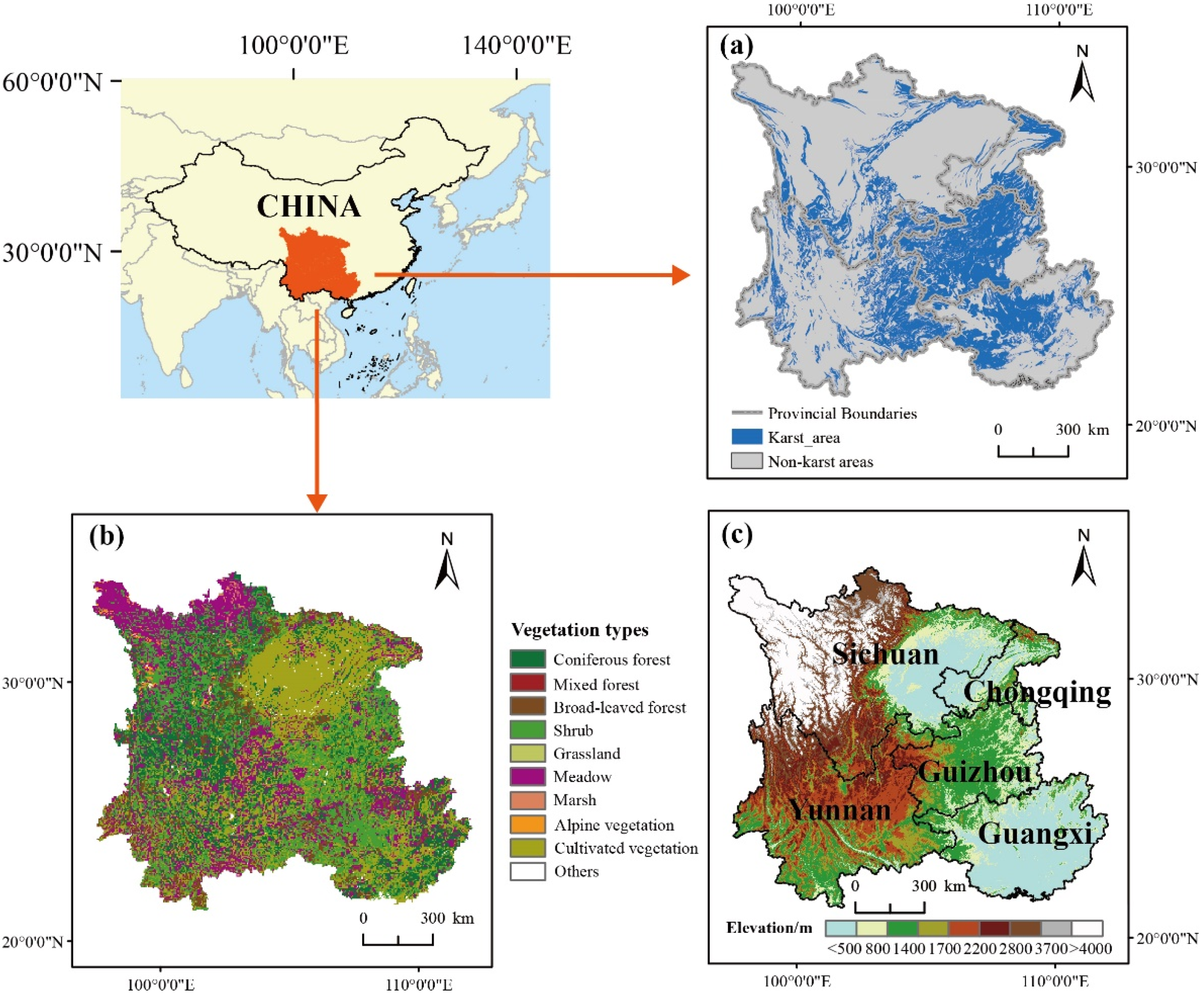
2.1. Study Area
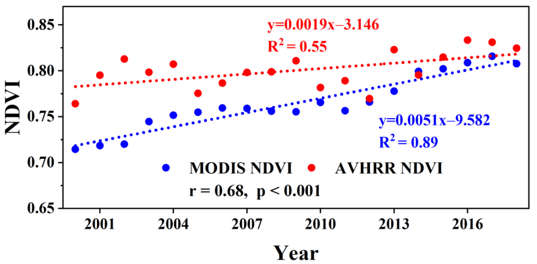
2.2. Data
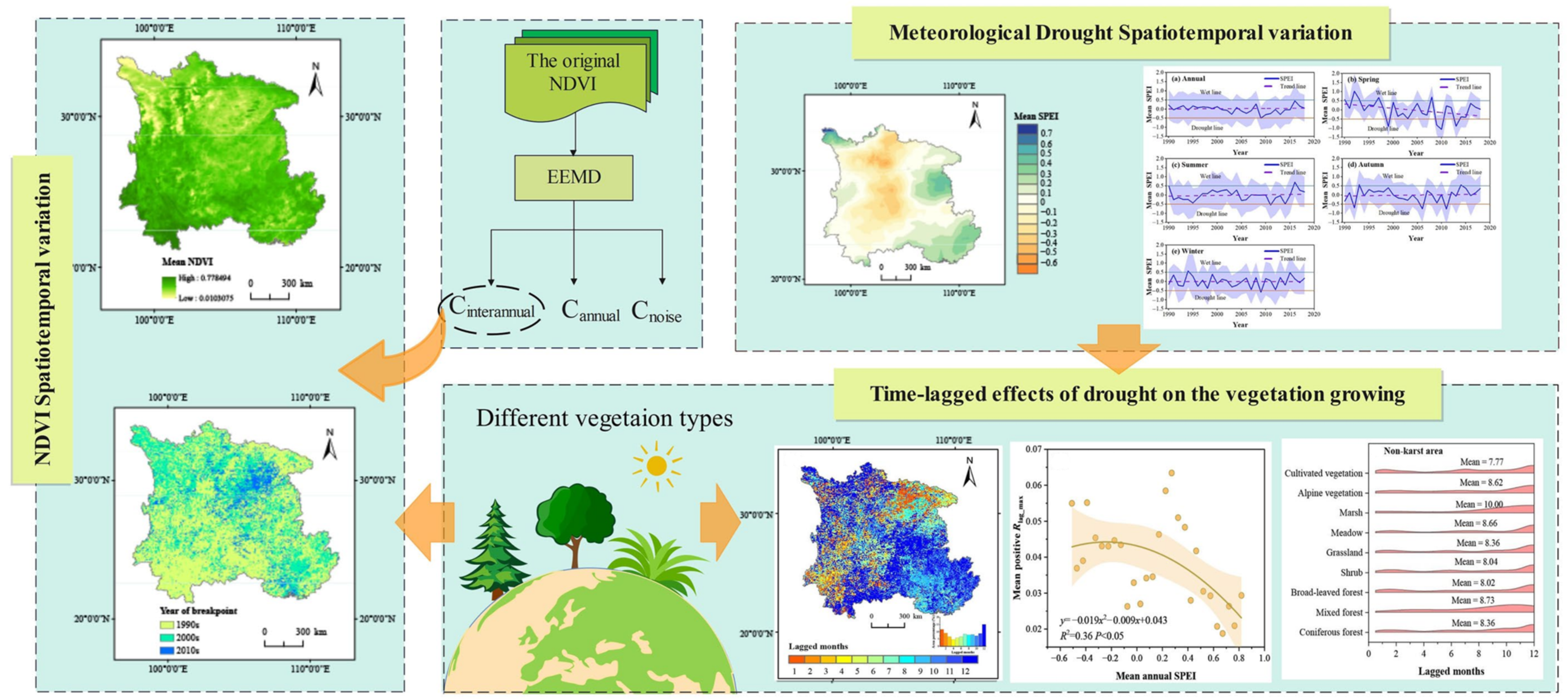
2.3. Methodology
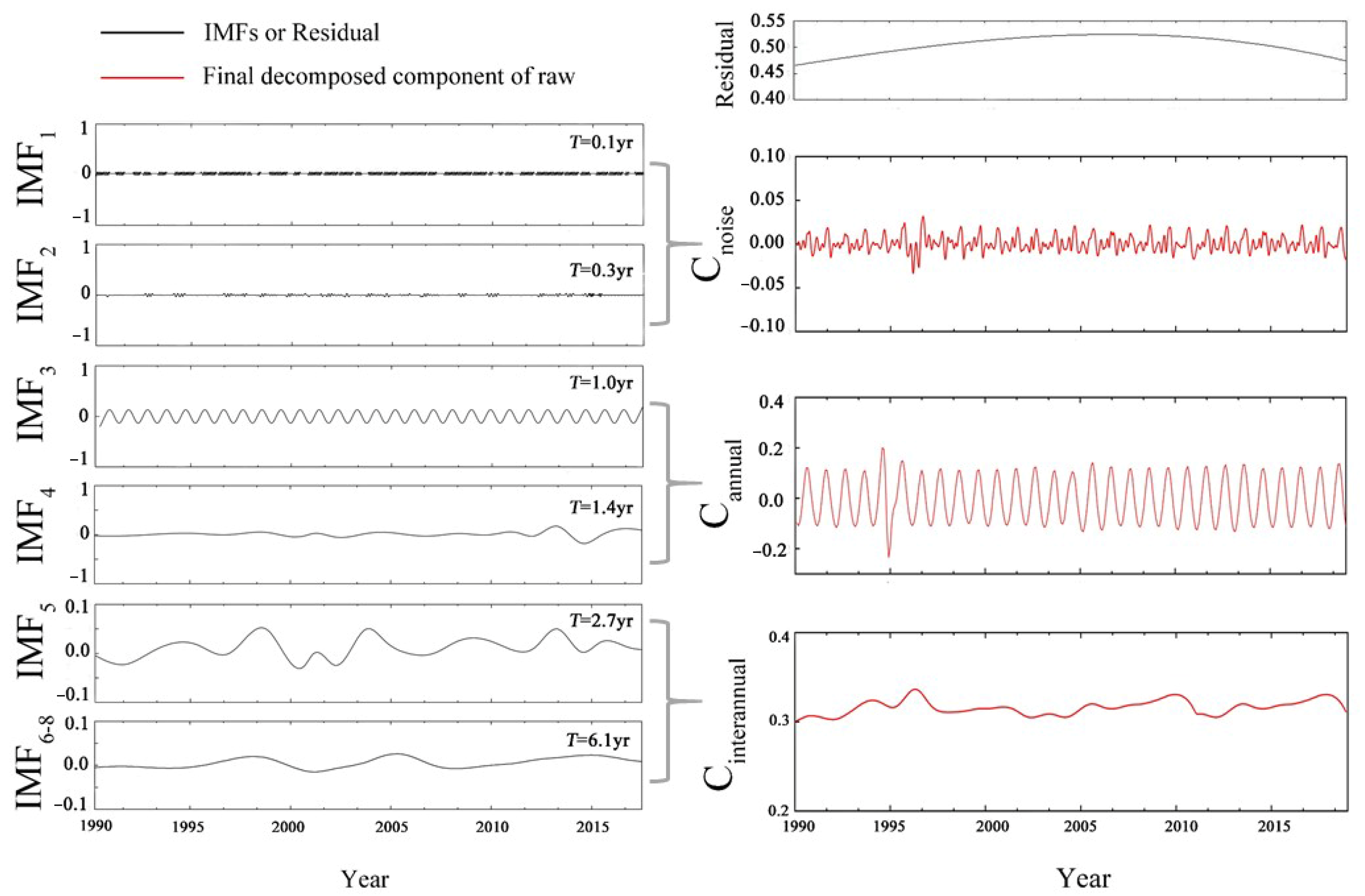
2.3.1. Reconstructing NDVI Time-Series Based on EEMD
2.3.2. Analyzing Linear and Nonlinear Trends in Interannual NDVI
2.3.3. Calculating Standardized Precipitation and Evapotranspiration Index (SPEI)
2.3.4. Determining the Time-Lagged Effect of Drought on Vegetation
3. Results
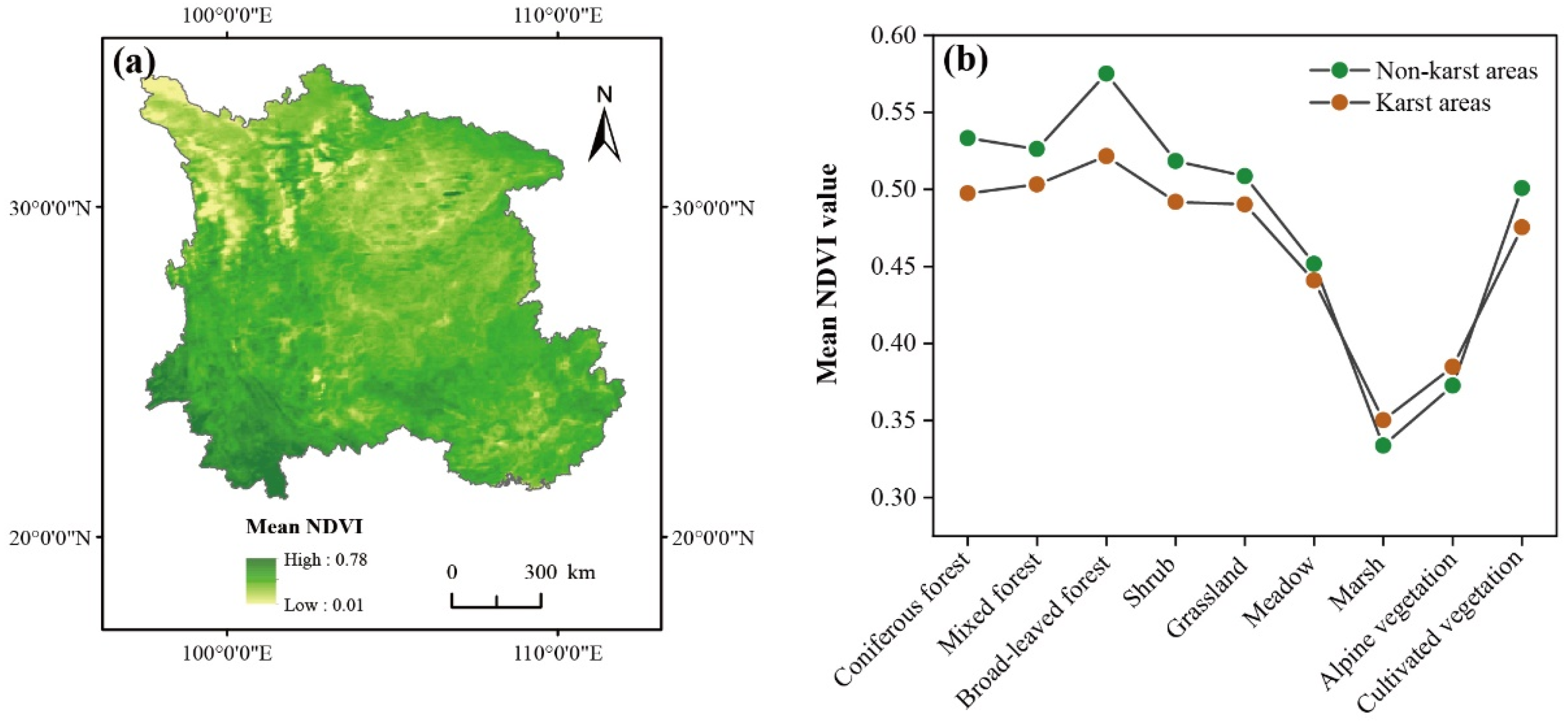
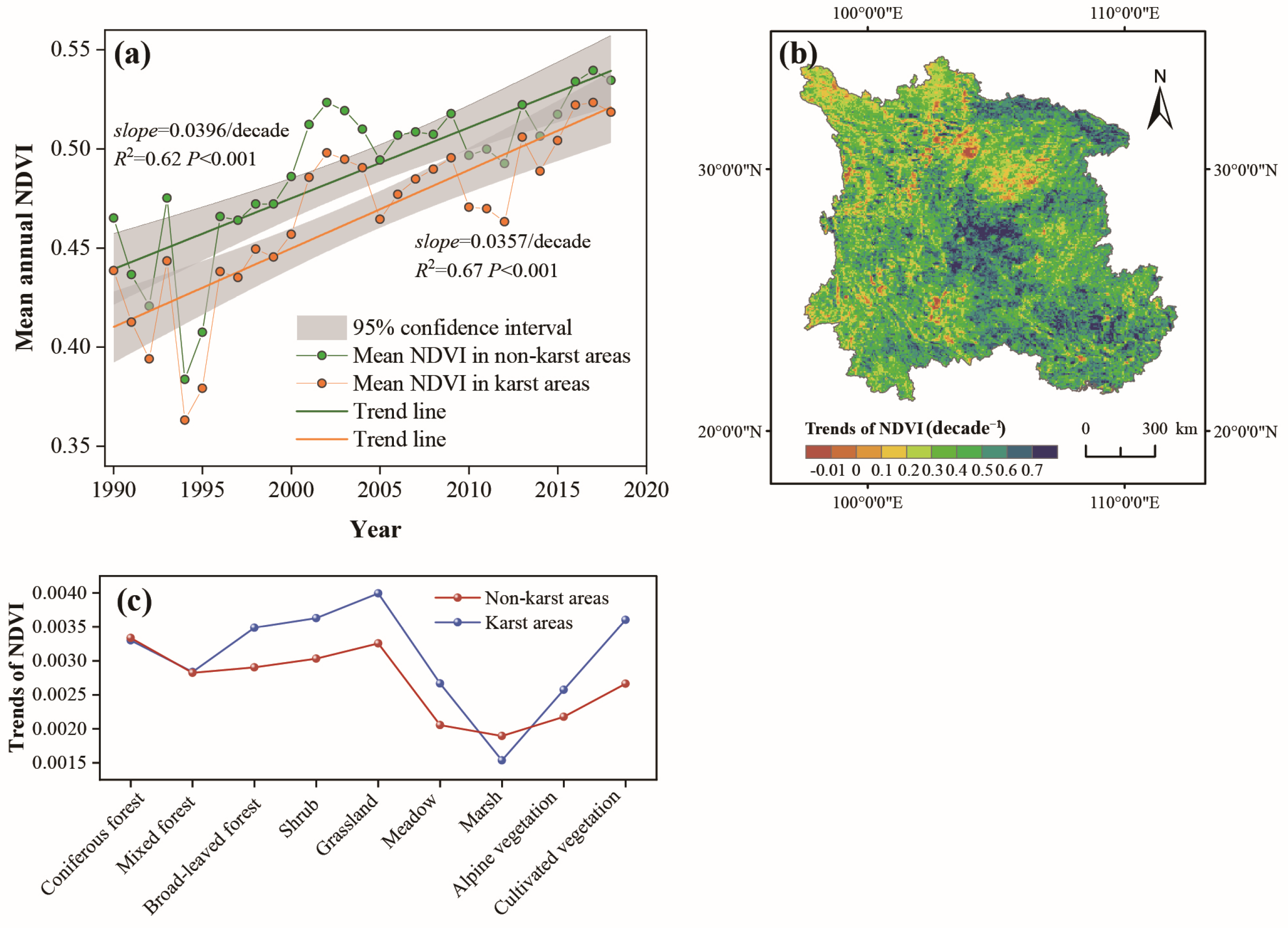
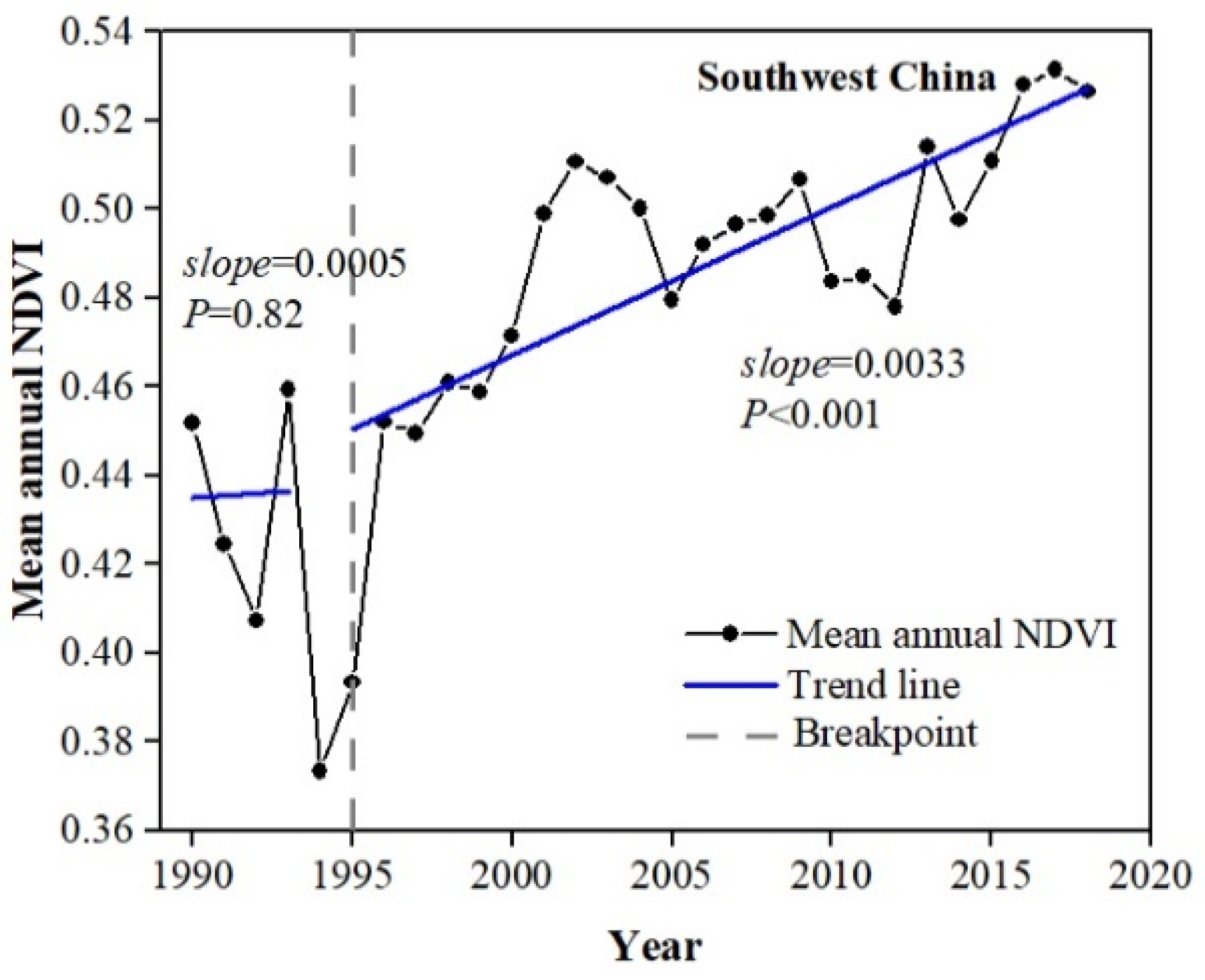
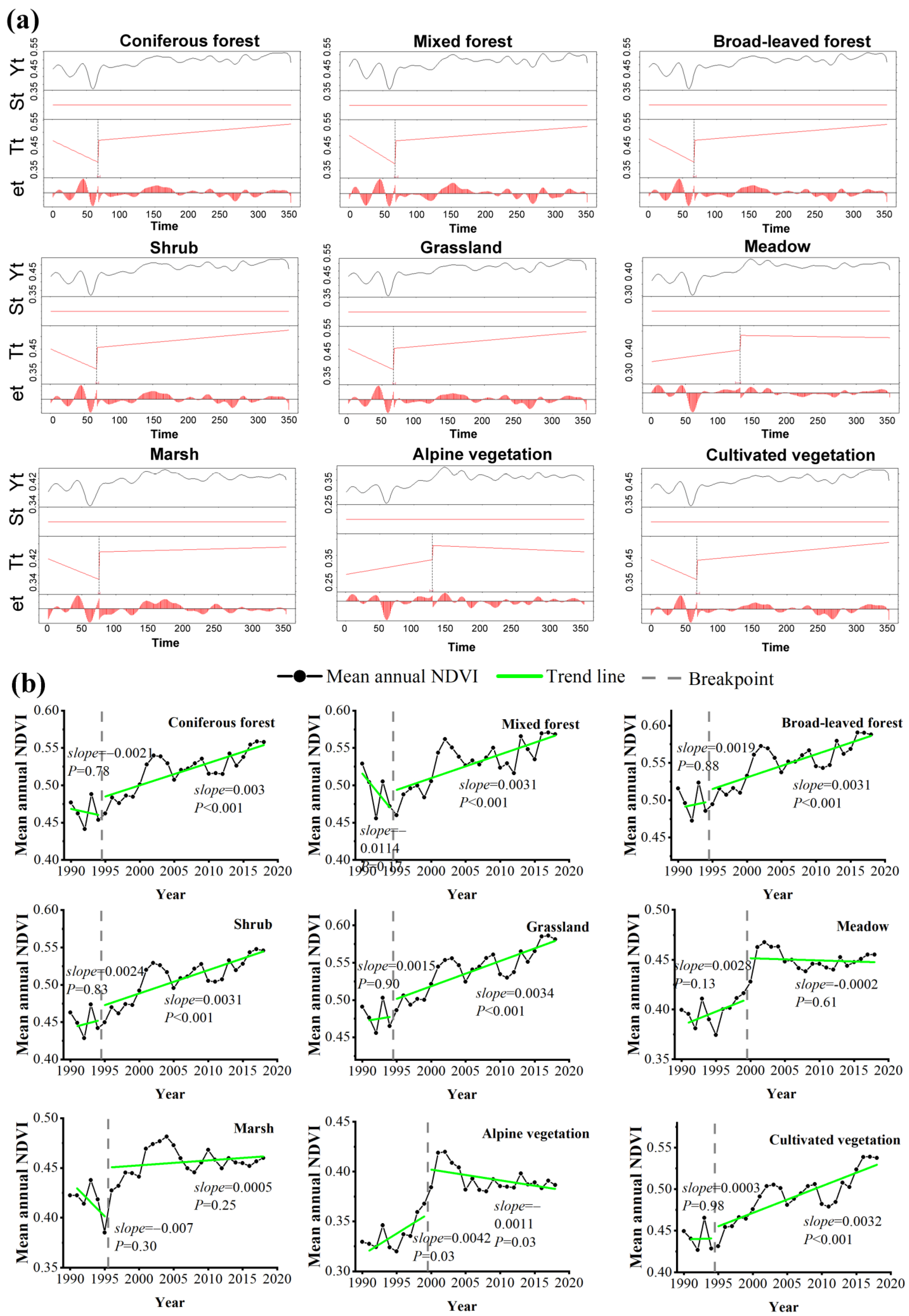
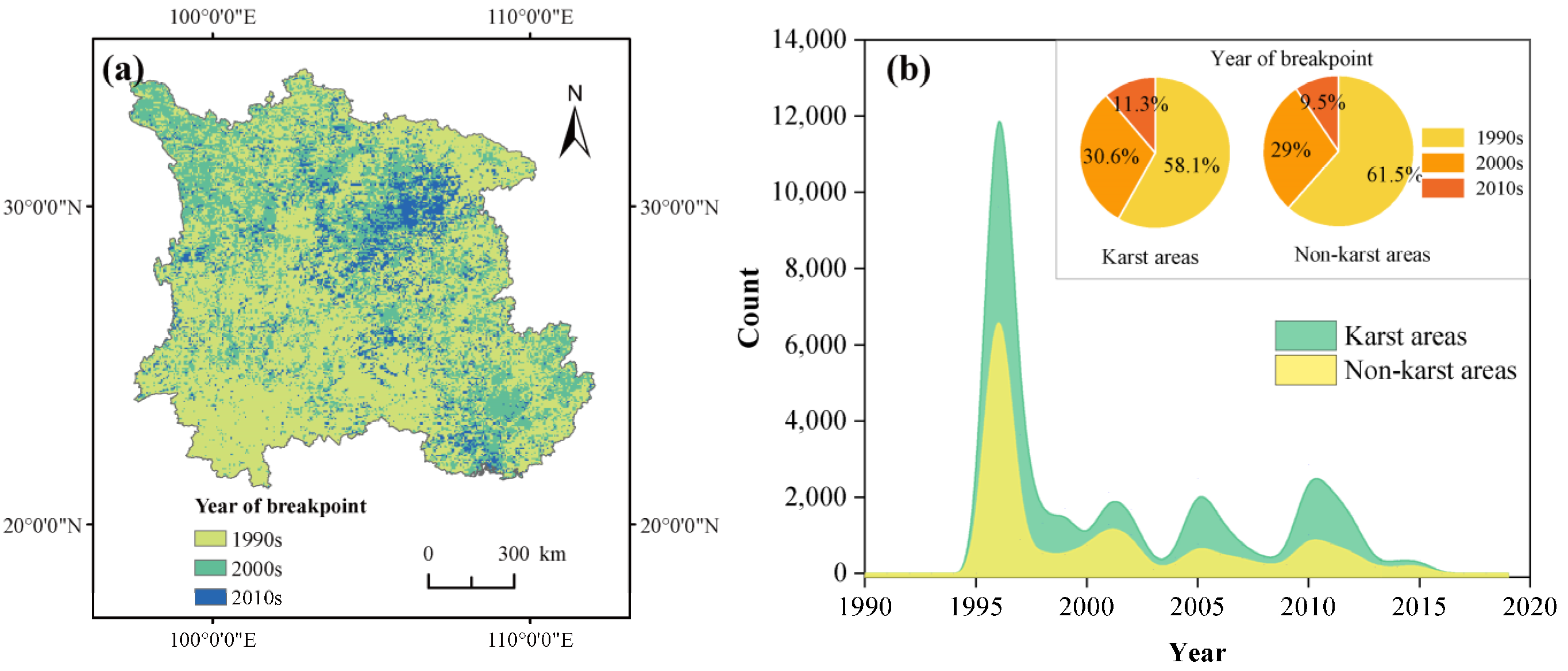
3.1. Spatiotemporal Variations and Abrupt Change in Vegetation Growth
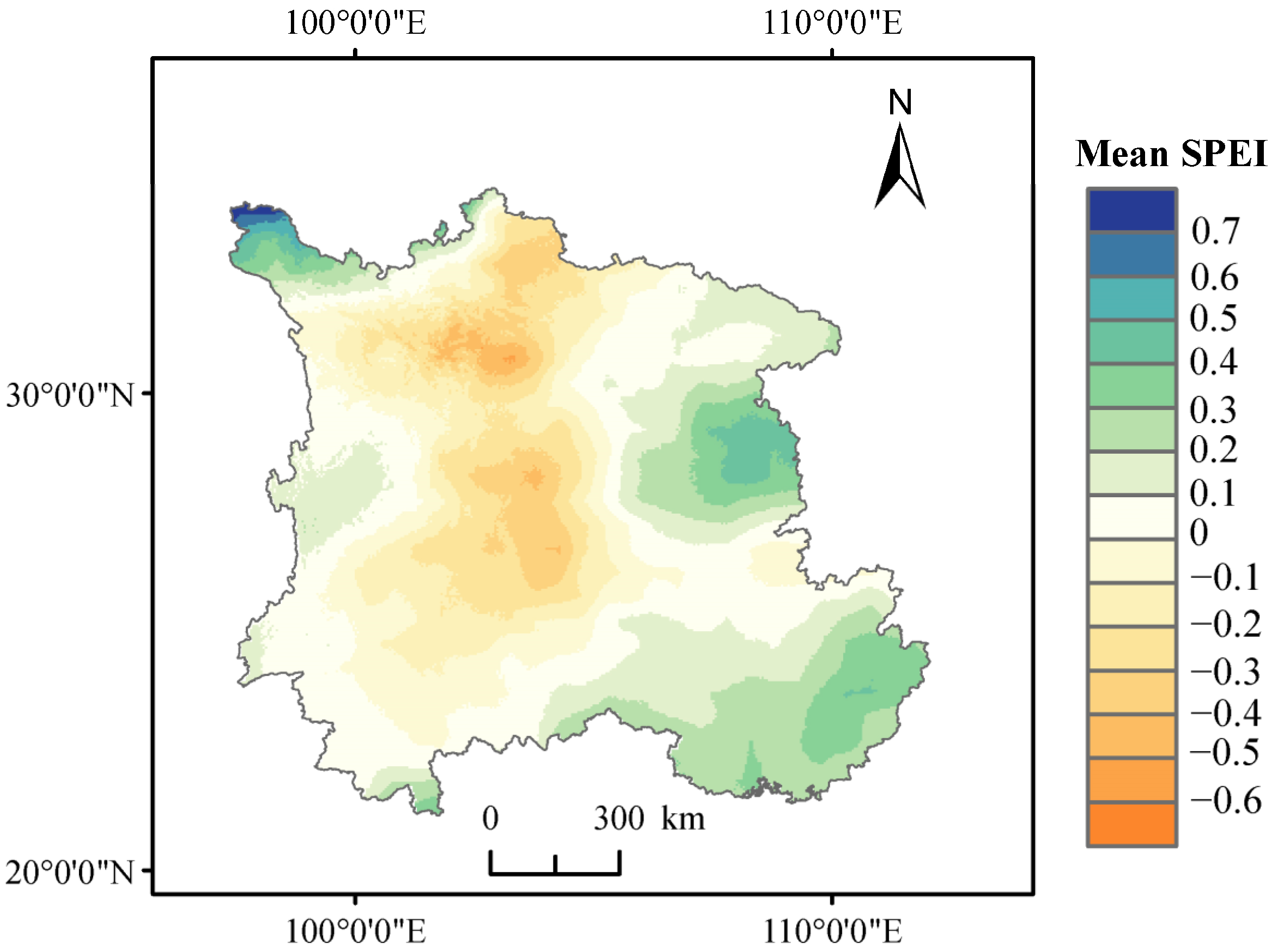
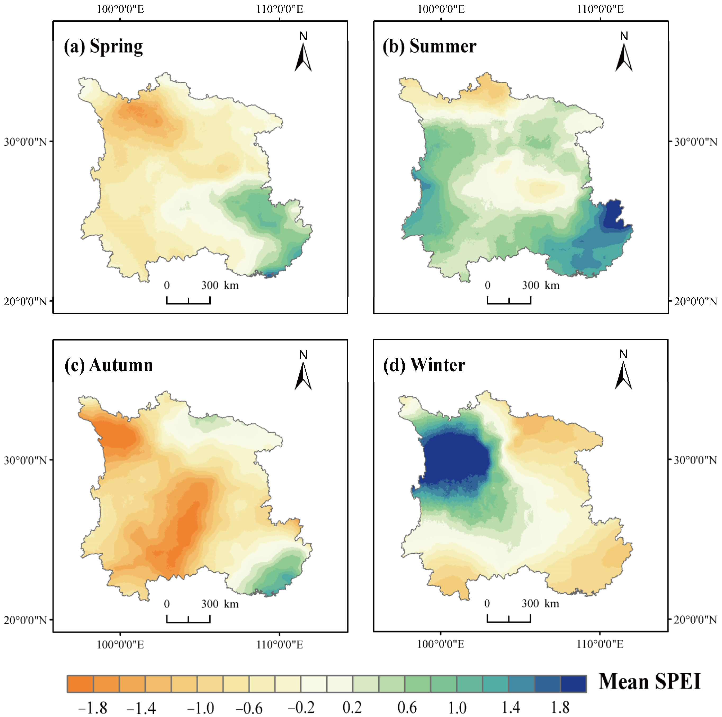
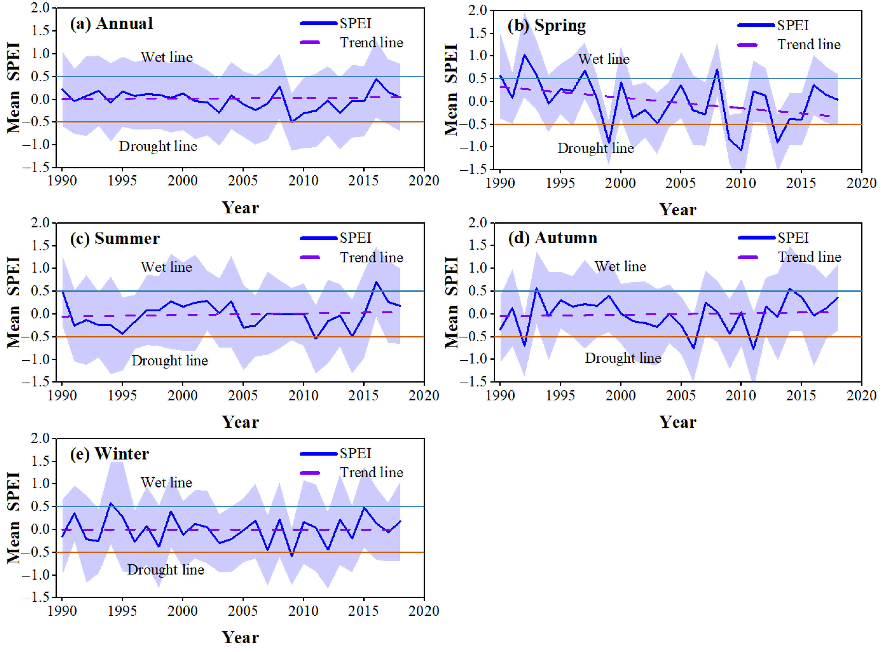
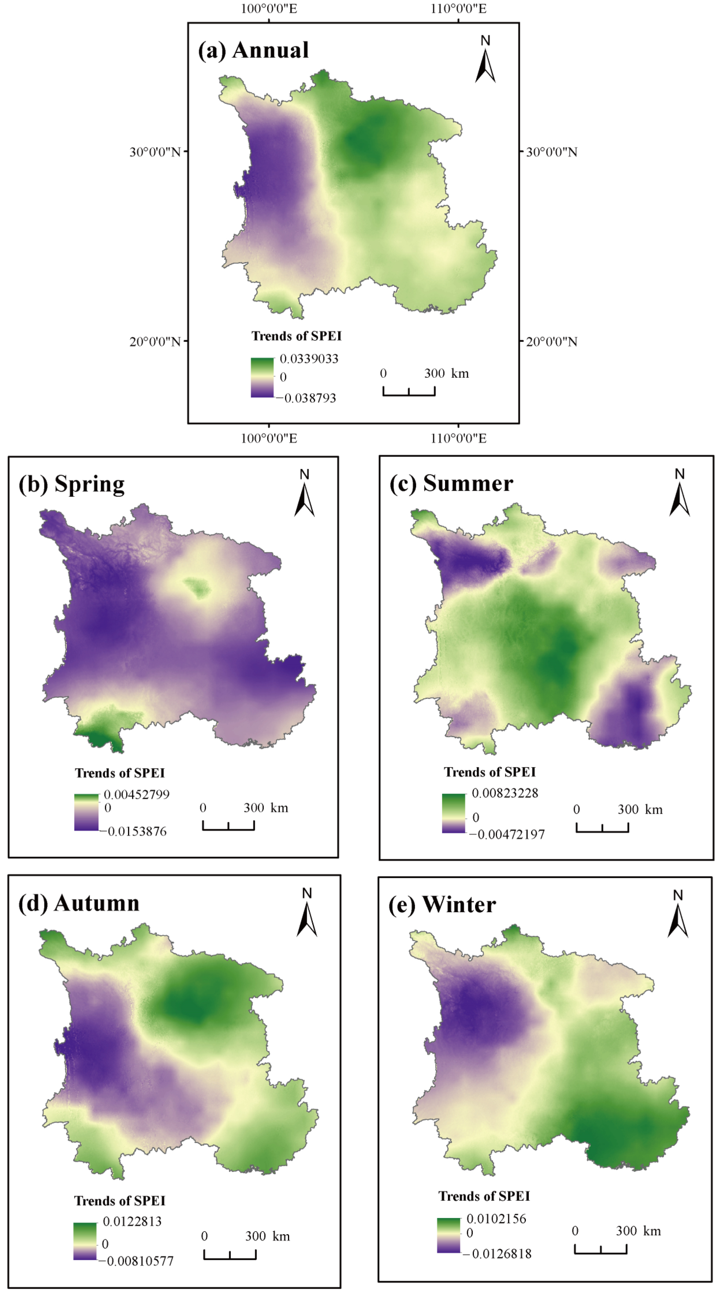
3.2. Meteorological Drought Spatiotemporal Changes
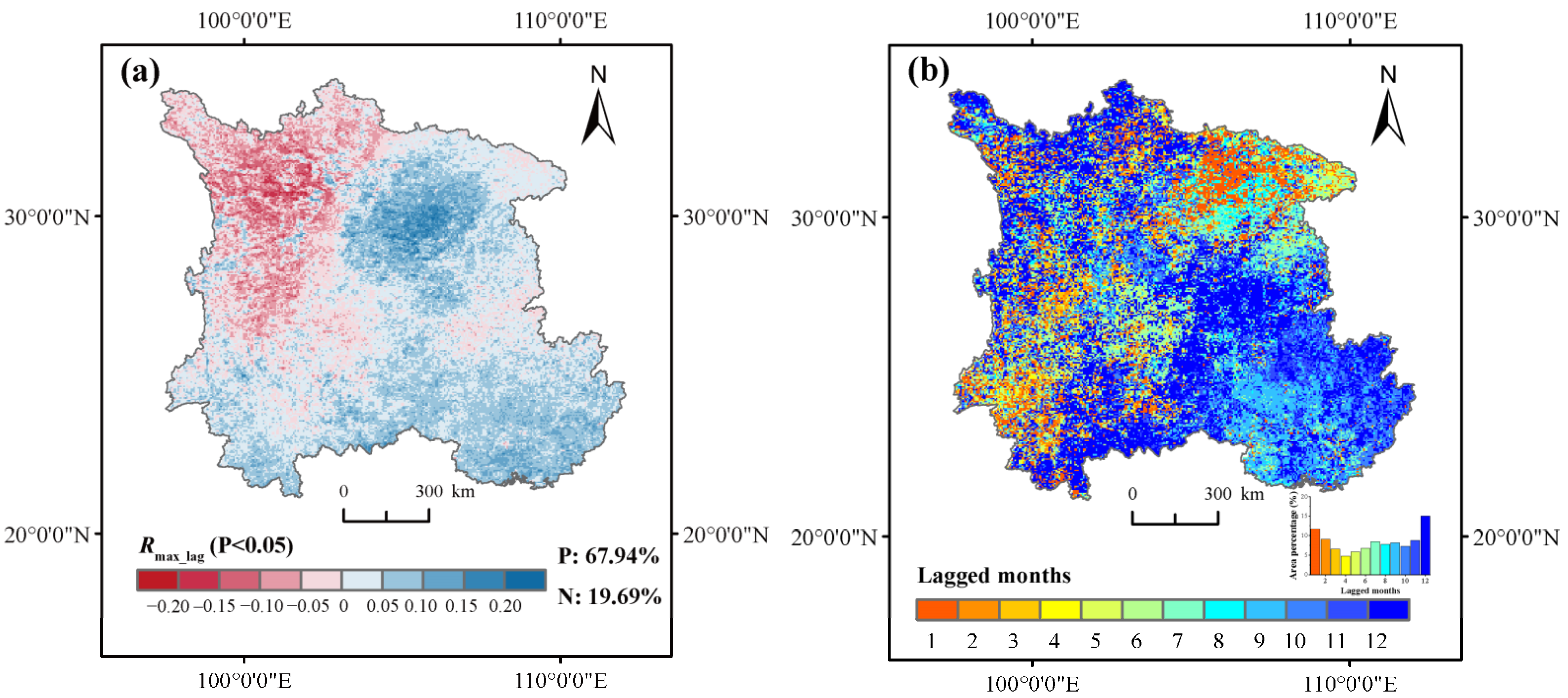
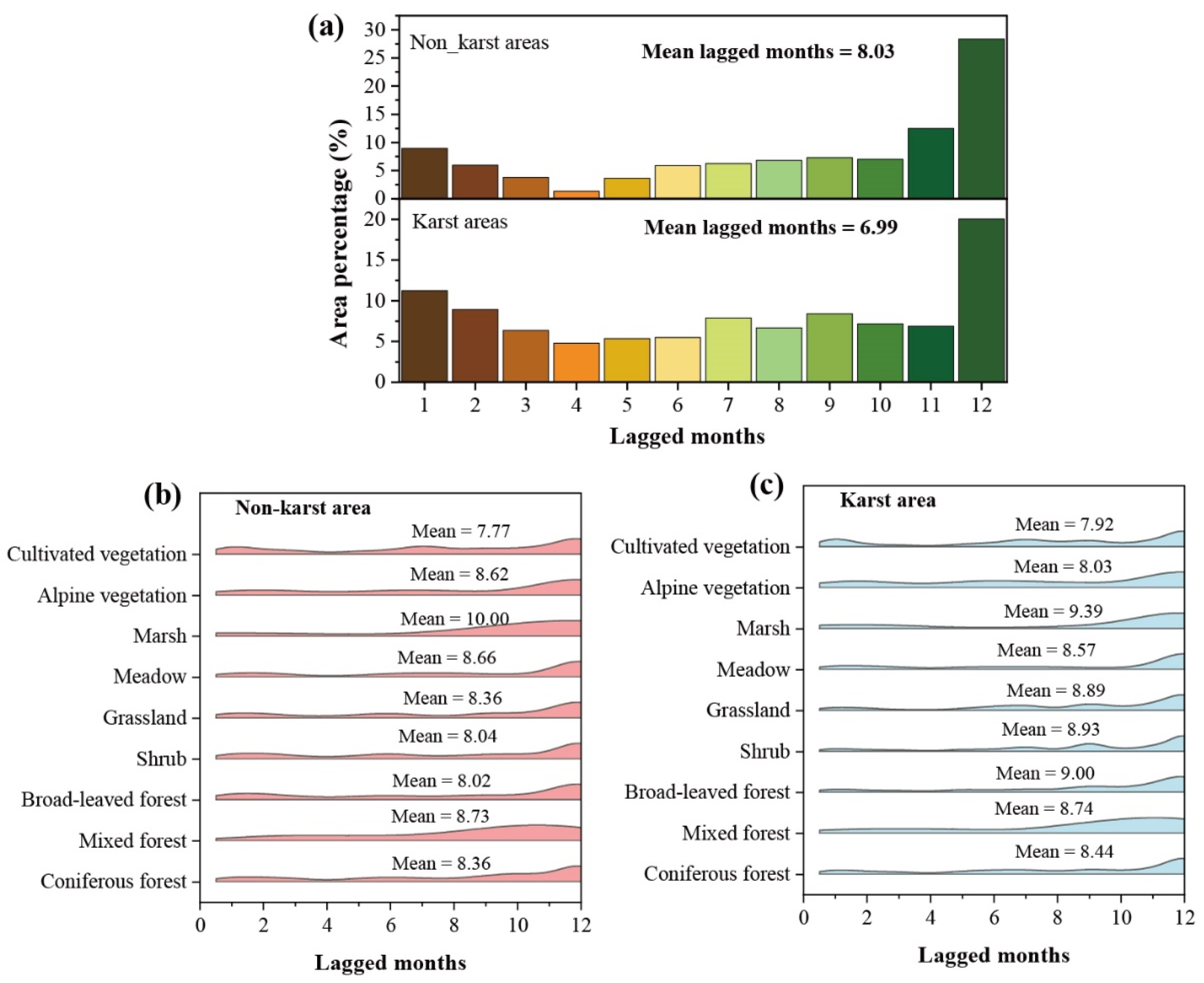
3.3. Time-Lagged Effect of Drought on Vegetation
4. Discussion
5. Conclusions
Author Contributions
Funding
Institutional Review Board Statement
Informed Consent Statement
Data Availability Statement
Acknowledgments
Conflicts of Interest
References
- Wen, Z.F.; Wu, S.J.; Chen, J.L.; Lu, M.Q. NDVI indicated long-term interannual changes in vegetation activities and their responses to climatic and anthropogenic factors in the Three Gorges Reservoir Region, China. Sci. Total Environ. 2017, 574, 947–959. [Google Scholar] [CrossRef]
- Komatsu, K.J.; Avolio, M.L.; Lemoine, N.P.; Isbell, F.; Isbell, F.; Grman, E.; Houseman, G.R.; Koerner, S.E.; Johnson, D.S.; Wilcox, K.R.; et al. Global change effects on plant communities are magnified by time and the number of global change factors imposed. Proc. Natl. Acad. Sci. USA 2019, 116, 17867–17873. [Google Scholar] [CrossRef] [Green Version]
- Shi, Y.; Jin, N.; Ma, X.L.; Wu, B.Y.; He, Q.S.; Yue, C.; Yu, Q. Attribution of climate and human activities to vegetation change in China using machine learning techniques. Agric. For. Meteorol. 2020, 294, 108146. [Google Scholar] [CrossRef]
- Xu, L.; Samanta, A.; Costa, M.H.; Ganguly, S.; Nemani, R.R.; Myneni, R.B. Widespread decline in greenness of Amazonian vegetation due to the 2010 drought. Geophys. Res. Lett. 2011, 38, L07402. [Google Scholar] [CrossRef] [Green Version]
- De Jong, R.; Verbesselt, J.; Schaepman, M.E.; De Bruin, S. Trend changes in global greening and browning: Contribution of short-term trends to longer-term change. Global Chang. Biol. 2012, 18, 642–655. [Google Scholar] [CrossRef]
- Nouri, H.; Anderson, S.J.; Sutton, P.C.; Beecham, S.; Nagler, P.L.; Jarchow, C.J.; Roberts, D.A. NDVI, scale invariance and the modifiable areal unit problem: An assessment of vegetation in the Adelaide Parklands. Sci. Total Environ. 2017, 584, 11–18. [Google Scholar] [CrossRef] [PubMed]
- Yang, L.Q.; Guan, Q.Y.; Lin, J.K.; Tian, J.; Tan, Z.; Li, H.C. Evolution of NDVI secular trends and responses to climate change: A perspective from nonlinearity and nonstationarity characteristics. Remote Sens. Environ. 2021, 254, 112247. [Google Scholar] [CrossRef]
- Zhang, Y.; Gentine, P.; Luo, X.Z.; Lian, X.; Liu, Y.L.; Zhou, S.; Michalak, A.M.; Sun, W.; Fisher, J.B.; Piao, S.L.; et al. Increasing sensitivity of dryland vegetation greenness to precipitation due to rising atmospheric CO2. Nat. Commun. 2022, 13, 4875. [Google Scholar] [CrossRef]
- Sha, Z.Y.; Bai, Y.F.; Li, R.R.; Lan, H.; Zhang, X.L.; Li, J.T.; Liu, X.F.; Chang, S.J.; Xie, Y.C. The global carbon sink potential of terrestrial vegetation can be increased substantially by optimal land management. Commun. Earth Environ. 2022, 3, 8. [Google Scholar] [CrossRef]
- Chen, C.; Park, T.; Wang, X.H.; Piao, S.L.; Xu, B.D.; Chaturvedi, R.K.; Fuchs, R.; Brovkin, V.; Ciais, P.; Fensholt, R. China and India lead in greening of the world through land-use management. Nat. Sustain. 2019, 2, 122–129. [Google Scholar] [CrossRef]
- Xue, S.Y.; Xu, H.Y.; Mu, C.C.; Wu, T.H.; Li, W.P.; Zhang, W.X.; Streletskaya, I.; Grebenets, V.; Sokratov, S.; Kizyakov, A.; et al. Changes in different land cover areas and NDVI values in northern latitudes from 1982 to 2015. Adv. Clim. Chang. Res. 2021, 12, 456–465. [Google Scholar] [CrossRef]
- Forzieri, G.; Dakos, V.; McDowell, N.G.; Ramdane, A.; Cescatti, A. Emerging signals of declining forest resilience under climate change. Nature 2022, 608, 534. [Google Scholar] [CrossRef] [PubMed]
- Smith, T.; Traxl, D.; Boers, N. Empirical evidence for recent global shifts in vegetation resilience. Nat. Clim. Chang. 2022, 12, 477. [Google Scholar] [CrossRef]
- Nunes, C.A.; Berenguer, E.; Frana, F.; Ferreira, J.; Lees, A.C.; Louzada, J.; Sayer, E.; Solar, R.; Smth, C.C.; Aragao, L.E.O.C.; et al. Linking land-use and land-cover transitions to their ecological impact in the Amazon. Proc. Natl. Acad. Sci. USA 2022, 119, e2202310119. [Google Scholar] [CrossRef] [PubMed]
- Song, X.P.; Hansen, M.C.; Stehman, S.V.; Potapov, P.V.; Tyukavina, A.; Vermote, E.F.; Townshend, J.R. Global land change from 1982 to 2016. Nature 2018, 563, E26. [Google Scholar] [CrossRef] [Green Version]
- Yang, Y.J.; Wang, S.J.; Bai, X.Y.; Tan, Q.; Li, Q.; Wu, L.H.; Tian, S.Q.; Hu, Z.Y.; Li, C.J.; Deng, Y.H. Factors Affecting Long-Term Trends in Global NDVI. Forests 2019, 10, 372. [Google Scholar] [CrossRef] [Green Version]
- Pasquarella, V.J.; Arevalo, P.; Bratley, K.H.; Bullock, E.L.; Gorelick, N.; Yang, Z.Q.; Kennedy, R.E. Demystifying LandTrendr and CCDC temporal segmentation. Int. J. Appl. Earth Obs. 2022, 110, 102806. [Google Scholar] [CrossRef]
- Diao, J.J.; Feng, T.; Li, M.S.; Zhu, Z.L.; Liu, J.X.; Biging, G.; Zheng, G.; Shen, W.J.; Wang, H.; Wang, J.R.; et al. Use of vegetation change tracker, spatial analysis, and random forest regression to assess the evolution of plantation stand age in Southeast China. Ann. Forest Sci. 2020, 77, 27. [Google Scholar] [CrossRef]
- Browning, D.M.; Maynard, J.J.; Karl, J.W.; Peters, D.C. Breaks in MODIS time series portend vegetation change: Verification using long-term data in an arid grassland ecosystem. Ecol. Appl. 2017, 27, 1677–1693. [Google Scholar] [CrossRef]
- Jamali, S.; Jonsson, P.; Eklundh, L.; Ardo, J.; Seaquist, J. Detecting changes in vegetation trends using time series segmentation. Remote Sens. Environ. 2015, 156, 182–195. [Google Scholar] [CrossRef]
- Verbesselt, J.; Hyndman, R.; Zeileis, A.; Culvenor, D. Phenological change detection while accounting for abrupt and gradual trends in satellite image time series. Remote Sens. Environ. 2010, 114, 2970–2980. [Google Scholar] [CrossRef] [Green Version]
- Ma, J.N.; Zhang, C.; Guo, H.; Chen, W.L.; Yun, W.J.; Gao, L.L.; Wang, H. Analyzing Ecological Vulnerability and Vegetation Phenology Response Using NDVI Time Series Data and the BFAST Algorithm. Remote Sens. 2020, 12, 3371. [Google Scholar] [CrossRef]
- Pan, N.Q.; Feng, X.M.; Fu, B.J.; Wang, S.; Ji, F.; Pan, S.F. Increasing global vegetation browning hidden in overall vegetation greening: Insights from time-varying trends. Remote Sens. Environ. 2018, 214, 59–72. [Google Scholar] [CrossRef]
- Hawinkel, P.; Swinnen, E.; Lhermitte, S.; Verbist, B.; Van Orshoven, J.; Muys, B. A time series processing tool to extract climate-driven interannual vegetation dynamics using Ensemble Empirical Mode Decomposition (EEMD). Remote Sens. Environ. 2015, 169, 375–389. [Google Scholar] [CrossRef] [Green Version]
- Kong, Y.L.; Meng, Y.; Li, W.; Yue, A.Z.; Yuan, Y. Satellite Image Time Series Decomposition Based on EEMD. Remote Sens. 2015, 7, 15583–15604. [Google Scholar] [CrossRef] [Green Version]
- Xue, P.; Liu, H.Y.; Zhang, M.Y.; Gong, H.B.; Cao, L. Nonlinear Characteristics of NPP Based on Ensemble Empirical Mode Decomposition from 1982 to 2015-A Case Study of Six Coastal Provinces in Southeast China. Remote Sens. 2022, 14, 15. [Google Scholar] [CrossRef]
- Mcdowell, N.G.; Sapes, G.; Pivovaroff, A.; Adams, H.D.; Allen, D.; Anderegg, W.R.L.; Arend, M.; Breshears, D.D.; Brodribb, T.L.; Choat, B.; et al. Mechanisms of woody-plant mortality under rising drought, CO2 and vapour pressure deficit. Nat. Rev. Earth Environ. 2022, 3, 294–308. [Google Scholar] [CrossRef]
- Deng, Y.; Wang, X.H.; Wang, K.; Ciais, P.; Tang, S.C.; Jin, L.; Li, L.L.; Piao, S.L. Responses of vegetation greenness and carbon cycle to extreme droughts in China. Agric. For. Meteorol. 2021, 298–299, 108307. [Google Scholar] [CrossRef]
- Zampieri, M.; Ceglar, A.; Dentener, F.; Toreti, A. Wheat yield loss attributable to heat waves, drought and water excess at the global, national and subnational scales. Environ. Res. Lett. 2017, 12, 64008. [Google Scholar] [CrossRef]
- Rashid, I.; Majeed, U.; Najar, N.A.; Bhat, I.A. Retreat of Machoi glacier, Kashmir Himalaya between 1972 and 2019 using remote sensing methods and field observations. Sci. Total Environ. 2021, 785, 147376. [Google Scholar] [CrossRef]
- Tang, W.X.; Liu, S.G.; Kang, P.; Peng, X.; Li, Y.Y.; Guo, R.; Jia, J.N.; Liu, M.C.; Zhu, L.J. Quantifying the lagged effects of climate factors on vegetation growth in 32 major cities of China. Ecol. Indic. 2021, 132, 108290. [Google Scholar] [CrossRef]
- Wu, D.H.; Zhao, X.; Liang, S.L.; Zhou, T.; Huang, K.C.; Tang, B.J.; Zhao, W.Q. Time-lag effects of global vegetation responses to climate change. Global Chang. Biol. 2015, 21, 3520–3531. [Google Scholar] [CrossRef]
- Wei, X.N.; He, W.; Zhou, Y.L.; Ju, W.M.; Xiao, J.F.; Li, X.; Liu, Y.B.; Xu, S.H.; Bi, W.J.; Zhang, X.Y.; et al. Global assessment of lagged and cumulative effects of drought on grassland gross primary production. Ecol. Indic. 2022, 136, 108646. [Google Scholar] [CrossRef]
- Zhao, A.Z.; Yu, Q.Y.; Feng, L.L.; Zhang, A.B.; Pei, T. Evaluating the cumulative and time-lag effects of drought on grassland vegetation: A case study in the Chinese Loess Plateau. J. Environ. Manag. 2020, 261, 110214. [Google Scholar] [CrossRef]
- Anderegg, W.R.L.; Schwalm, C.; Biondi, F.; Camarero, J.J.; Koch, G.; Litvak, M.; Ogle, K.; Shaw, J.F.; Shevliakova, E.; Williams, A.P.; et al. Pervasive Drought Legacy Effects in Forest Ecosystems and their Carbon Cycle Implications. Science 2015, 349, 528–532. [Google Scholar] [CrossRef] [PubMed] [Green Version]
- Tong, X.W.; Brandt, M.; Yue, Y.M.; Horion, S.; Wang, K.L.; De Keersmaecker, K.; Tian, F.; Schurgers, G.; Xiao, X.M.; Luo, Y.Q.; et al. Increased vegetation growth and carbon stock in China karst via ecological engineering. Nat. Sustain. 2018, 1, 44–50. [Google Scholar] [CrossRef]
- Zhang, X.M.; Brandt, M.; Yue, Y.M.; Tong, X.W.; Wang, K.L.; Fensholt, R. The Carbon Sink Potential of Southern China After Two Decades of Afforestation. Earth’s Future 2022, 10, e2022EF002674. [Google Scholar] [CrossRef] [PubMed]
- Liu, Y.Y.; Hu, Z.Z.; Wu, R.G.; Yuan, X. Causes and Predictability of the 2021 Spring Southwestern China Severe Drought. Adv. Atmos. Sci. 2022, 39, 1766–1776. [Google Scholar] [CrossRef]
- Feng, Q.; Zhou, Z.F.; Zhu, C.L.; Luo, W.L.; Zhang, L. Quantifying the Ecological Effectiveness of Poverty Alleviation Relocation in Karst Areas. Remote Sens. 2022, 14, 5920. [Google Scholar] [CrossRef]
- Peng, D.W.; Zhou, Q.W.; Tang, X.; Yan, W.H.; Chen, M. Changes in soil moisture caused solely by vegetation restoration in the karst region of southwest China. J. Hydrol. 2022, 613, 128460. [Google Scholar] [CrossRef]
- Song, Z.H.; Xia, J.; She, D.X.; Li, L.C.; Hu, C.; Hong, S. Assessment of meteorological drought change in the 21st century based on CMIP6 multi-model ensemble projections over mainland China. J. Hydrol. 2021, 601, 126643. [Google Scholar] [CrossRef]
- Cheng, Q.P.; Gao, L.; Zhong, F.L.; Zuo, X.A.; Ma, M.M. Spatiotemporal variations of drought in the Yunnan-Guizhou Plateau, southwest China, during 1960–2013 and their association with large-scale circulations and historical records. Ecol. Indic. 2020, 112, 106041. [Google Scholar] [CrossRef]
- Wang, K.L.; Zhang, C.H.; Chen, H.S.; Yue, Y.M.; Zhang, W.; Zhang, M.Y.; Qi, X.K.; Fu, Z.Y. Karst landscapes of China: Patterns, ecosystem processes and services. Landsc. Ecol. 2019, 34, 2743–2763. [Google Scholar] [CrossRef] [Green Version]
- NOAA CDR Program NOAA Climate Data Record (CDR) of AVHRR Normalized Difference Vegetation Index (NDVI), Version 5. Available online: http://www.geodata.cn (accessed on 21 September 2022).
- Holben, N.B. Characteristics of maximum-value composite images from temporal AVHRR data. Int. J. Remote Sens. 1986, 7, 1417–1434. [Google Scholar] [CrossRef]
- Fensholt, R.; Proud, S.R. Evaluation of earth observation based global long term vegetation trends—Comparing GIMMS and MODIS global NDVI time series. Remote Sens. Environ. 2012, 119, 131–147. [Google Scholar] [CrossRef]
- Tian, F.; Fensholt, R.; Verbesselt, J.; Grogan, K.; Horion, S.; Wang, Y.J. Evaluating temporal consistency of long-term global NDVI datasets for trend analysis. Remote Sens. Environ. 2015, 163, 326–340. [Google Scholar] [CrossRef]
- 1-km Monthly Mean Temperature Dataset for China (1901–2021). Available online: http://data.tpdc.ac.cn/zh-hans/ (accessed on 22 August 2022).
- Peng, S.Z.; Ding, Y.X.; Liu, W.Z.; Li, Z. 1 km monthly temperature and precipitation dataset for China from 1901 to 2017. Earth Syst. Sci. Data 2019, 11, 1931–1946. [Google Scholar] [CrossRef] [Green Version]
- McColl, K.A. Practical and Theoretical Benefits of an Alternative to the Penman-Monteith Evapotranspiration Equation. Water Resour. Res. 2020, 56, e2020WR027106. [Google Scholar] [CrossRef]
- Proutsos, N.D.; Tsiros, I.X.; Nastos, P.; Tsaousidis, A. A note on some uncertainties associated with Thornthwaite’s aridity index introduced by using different potential evapotranspiration methods. Atmos. Res. 2021, 260, 105727. [Google Scholar] [CrossRef]
- Hargreaves, G.H.; Allen, R.G. History and evaluation of Hargreaves evapotranspiration equation. J. Irrig. Drain. Eng. 2003, 129, 53–63. [Google Scholar] [CrossRef]
- Su, Y.J.; Guo, Q.H.; Hu, T.Y.; Guan, H.C.; Jin, S.C.; An, S.Z.; Chen, X.L.; Guo, K.; Hao, Z.Q.; Hu, Y.M.; et al. An updated Vegetation Map of China (1:1000000). Sci. Bull. 2020, 65, 1125–1136. [Google Scholar] [CrossRef]
- Wu, Z.H.; Huang, N.E. Ensemble empirical mode decomposition: A noise-assisted data analysis method. Adv. Adapt. Data Anal. 2009, 1, 1793. [Google Scholar] [CrossRef]
- Lambert, J.; Drenou, C.; Denux, J.P.; Balent, G.; Cheret, V. Monitoring forest decline through remote sensing time series analysis. Gisci. Remote Sens. 2013, 50, 437–457. [Google Scholar]
- Vicente-Serrano, S.M.; Begueria, S.; Lopez-Moreno, J.I. A Multiscalar Drought Index Sensitive to Global Warming: The Standardized Precipitation Evapotranspiration Index. J. Clim. 2010, 23, 1696–1718. [Google Scholar] [CrossRef] [Green Version]
- Peng, J.; Wu, C.Y.; Zhang, X.Y.; Wang, X.Y.; Gonsamo, A. Satellite detection of cumulative and lagged effects of drought on autumn leaf senescence over the Northern Hemisphere. Global Chang. Biol. 2019, 25, 2174–2188. [Google Scholar] [CrossRef]
- Jiang, S.S.; Chen, X.; Smettem, K.; Wang, T.J. Climate and land use influences on changing spatiotemporal patterns of mountain vegetation cover in southwest China. Ecol. Indic. 2021, 121, 107193. [Google Scholar] [CrossRef]
- Martin, B.; Yue, Y.M.; Wigneron, J.P.; Tong, X.W.; Tian, F.; Jepsen, M.R.; Xiao, X.M.; Verger, A.; Mialin, A.; Al-Yaari, A.; et al. Satellite-observed Major Greening and Biomass Increase in South China Karst During Recent Decade. Earth’s Future 2018, 6, 1017–1028. [Google Scholar]
- Yang, H.; Hu, J.; Zhang, S.; Xiong, L.; Xu, Y. Climate Variations vs. Human Activities: Distinguishing the Relative Roles on Vegetation Dynamics in the Three Karst Provinces of Southwest China. Front. Earth Sci. 2022, 10, 799493. [Google Scholar] [CrossRef]
- Chu, H.S.; Venevsky, S.; Wu, C.; Wang, M.H. NDVI-based vegetation dynamics and its response to climate changes at Amur-Heilongjiang River Basin from 1982 to 2015. Sci. Total Environ. 2018, 650, 2051–2062. [Google Scholar] [CrossRef]
- Ding, Z.; Zheng, H.; Liu, Y.; Zeng, S.D.; Yu, P.J.; Shi, W.; Tang, X.G. Spatiotemporal Patterns of Ecosystem Restoration Activities and Their Effects on Changes in Terrestrial Gross Primary Production in Southwest China. Remote Sens. 2021, 13, 1209. [Google Scholar] [CrossRef]
- Li, Y.J.; Ren, F.M.; Li, Y.P.; Wang, P.L.; Yan, H.M. Characteristics of the Regional Meteorological Drought Events in Southwest China During 1960–2010. J. Meteorol. Res. 2014, 28, 381–392. [Google Scholar] [CrossRef]
- Wang, L.; Chen, W.; Zhou, W.; Huang, G. Understanding and detecting super-extreme droughts in Southwest China through an integrated approach and index. Q. J. R. Meteorol. Soc. 2016, 142, 529–535. [Google Scholar] [CrossRef]
- Sun, H.; Wang, X.P.; Fan, D.Y.; Sun, O.J.X. Contrasting vegetation response to climate change between two monsoon regions in Southwest China: The roles of climate condition and vegetation height. Sci. Total Environ. 2021, 802, 149643. [Google Scholar] [CrossRef]
- Li, G.; Li, C.Y.; Zhou, W.; Wen, B. Climatic Characteristics of Rainfall over Southwest China during Spring and Spring Months. Clim. Environ. Res. 2020, 25, 575–587. [Google Scholar]
- Mei, S.L.; Chen, S.F.; Li, Y.; Aru, H. Interannual Variations of Rainfall in Late Spring over Southwest China and Associated Sea Surface Temperature and Atmospheric Circulation Anomalies. Atmosphere 2022, 13, 735. [Google Scholar] [CrossRef]
- Zhang, L.; Xiao, J.F.; Li, J.; Wang, K.; Lei, L.P.; Guo, H.D. The 2010 spring drought reduced primary productivity in southwestern China. Environ. Res. Lett. 2012, 7, 045706. [Google Scholar] [CrossRef] [Green Version]
- Lian, X.; Piao, S.L.; Li, L.Z.X.; Li, Y.; Huntingford, C.; Cuais, P.; Cescatti, A.; Janssens, I.A.; Penuela, J.; Buermann, W.; et al. Summer soil drying exacerbated by earlier spring greening of northern vegetation. Sci. Adv. 2020, 6, eaax0255. [Google Scholar] [CrossRef] [Green Version]
- Xu, X.J.; Liu, H.Y.; Lin, Z.S.; Jiao, F.S.; Gong, H.B. Relationship of Abrupt Vegetation Change to Climate Change and Ecological Engineering with Multi-Timescale Analysis in the Karst Region, Southwest China. Remote Sens. 2019, 11, 1564. [Google Scholar] [CrossRef] [Green Version]
- Vicente-Serrano, S.M.; Gouveia, C.; Camarero, J.J.; Begueria, S.; Trigo, R.; Lopez-Moreno, J.I.; Azorin-Molina, C.; Pasho, E.; Lorenzo-Lacruz, J.; Revuelto, J.; et al. Response of vegetation to drought time-scales across global land biomes. Proc. Natl. Acad. Sci. USA 2013, 110, 52–57. [Google Scholar] [CrossRef] [Green Version]
- Yan, W.M.; Zhong, Y.Q.W.; Shangguan, Z.P. Responses of different physiological parameter thresholds to soil water availability in four plant species during prolonged drought. Agric. Forest Meteorol. 2017, 247, 311–319. [Google Scholar] [CrossRef]
- Ma, Z.Q.; Guo, D.L.; Xu, X.L.; Lu, M.Z.; Bardgett, R.D.; Eissenstat, D.M.; Mccormack, M.L.; Hedin, L.O. evolutionary history resolves global organization of root functional traits. Nature 2018, 555, 94–97. [Google Scholar] [CrossRef] [PubMed] [Green Version]
- Chen, W.; Bai, S.; Zhao, H.M.; Han, X.R.; Li, L.H. Spatiotemporal analysis and potential impact factors of vegetation variation in the karst region of Southwest China. Environ. Sci. Pollut. Res. 2021, 28, 61258–61273. [Google Scholar] [CrossRef]


| SPEI Values | Class |
|---|---|
| 0.5 ≤ SPEI | No drought |
| −0.5 ≤ SPEI < 0.5 | Semi-arid or semi humid |
| −1.0 ≤ SPEI < −0.5 | Mild drought |
| −1.5 ≤ SPEI < −1.0 | Moderate drought |
| SPEI ≤ −1.5 | Severe drought |
Disclaimer/Publisher’s Note: The statements, opinions and data contained in all publications are solely those of the individual author(s) and contributor(s) and not of MDPI and/or the editor(s). MDPI and/or the editor(s) disclaim responsibility for any injury to people or property resulting from any ideas, methods, instructions or products referred to in the content. |
© 2023 by the authors. Licensee MDPI, Basel, Switzerland. This article is an open access article distributed under the terms and conditions of the Creative Commons Attribution (CC BY) license (https://creativecommons.org/licenses/by/4.0/).
Share and Cite
Jiang, P.; Wang, Y.; Yang, Y.; Gu, X.; Huang, Y.; Liu, L.; Liu, L. Spatiotemporal Features and Time-Lagged Effects of Drought on Terrestrial Ecosystem in Southwest China. Forests 2023, 14, 781. https://doi.org/10.3390/f14040781
Jiang P, Wang Y, Yang Y, Gu X, Huang Y, Liu L, Liu L. Spatiotemporal Features and Time-Lagged Effects of Drought on Terrestrial Ecosystem in Southwest China. Forests. 2023; 14(4):781. https://doi.org/10.3390/f14040781
Chicago/Turabian StyleJiang, Pan, Yuxi Wang, Yang Yang, Xinchen Gu, Yi Huang, Lei Liu, and Liang Liu. 2023. "Spatiotemporal Features and Time-Lagged Effects of Drought on Terrestrial Ecosystem in Southwest China" Forests 14, no. 4: 781. https://doi.org/10.3390/f14040781