Forest Fire Prediction Based on Long- and Short-Term Time-Series Network

Abstract

Modeling and prediction of forest fire occurrence play a key role in guiding forest fire prevention. From the perspective of the whole world, forest fires are a natural disaster with a great degree of hazard, and many countries have taken mountain fire prediction as an important measure for fire prevention and control, and have conducted corresponding research. In this study, a forest fire prediction model based on LSTNet is proposed to improve the accuracy of forest fire forecasts. The factors that influence forest fires are obtained through remote sensing satellites and GIS, and their correlation is estimated using Pearson correlation analysis and testing for multicollinearity. To account for the spatial aggregation of forest fires, the data set was constructed using oversampling methods and proportional stratified sampling, and the LSTNet forest fire prediction model was established based on eight influential factors. Finally, the predicted data were incorporated into the model and the predicted risk map of forest fires in Chongli, China was drawn. This paper uses metrics such as RMSE to compare with traditional machine learning methods, and the results show that the LSTNet model proposed in this paper has high accuracy (ACC 0.941). This study illustrates that the model can effectively use spatial background information and the periodicity of forest fire factors, and is a novel method for spatial prediction of forest fire susceptibility.

1. Introduction

One of the most destructive natural disasters in the world, forest fires are distinguished by their extreme suddenness and difficulty in rescue. There are more than 100,000 forest fires around the world every year, and the burned forest area has reached more than 1 million hectares. In the past half-century in China, there have been more than 730,000 forest fires, and the burned forest area has reached more than 30 million hectares. Forest fires seriously endanger people’s lives and the security of their property, in addition to endangering the forest’s natural resources.

From a global perspective, forest fires usually do not occur in polar regions above 70 degrees north latitude and 70 degrees south latitude, and more and more occur in tropical regions. However, global climate change may have a far-reaching and unexpected impact on future global forest fire activity. The average length of the global forest fire season has increased by 20% in recent decades due to global warming [1,2], which has led to higher temperatures, more frequent droughts, and lower air humidity [3]. The spatial extent of the effects of forest fires has also increased [4,5], and both the frequency and intensity of forest fires are increasing globally [6,7]. As a result, there is a long-term risk of forest fires occurring anywhere in the world. Therefore, the development of forest fire prediction technology with high accuracy plays a huge role in forest fire early warning.

Traditional forest fire prediction is mainly divided into statistical-based empirical models and machine learning. Statistical-based methods include statistical analysis, fire for fire, and correlation methods. Statistical analysis is to collect meteorological data related to historical fires; statistically analyze meteorological factors such as weather conditions, time, terrain, and frequency of historical fires; determine the correlation between fires and various meteorological factors; and obtain the law of fire occurrence. Baranovskiy et al. [8] predicted the forest fire risk near the Russian railway through a computer program. Barmpoutis et al. [9] established a fire early warning model through optical remote sensing technology. Sakr et al. [10] used two weather parameters to effectively predict the occurrence of forest fires in developing countries. Pradeep et al. [11] used GIS to divide the forest fire danger zone in India’s Eravikulam National Park. A study found that river flow is a reliable indicator of forest fire risk in Tasmania Wilderness World Heritage Area in temperate Australia [12]. Gülçin et al. [13] drew the forest fire risk map of the Manisa area in Turkey based on GIS. Maffei et al. [14] combined multi-spectrum and thermal remote sensing to predict the characteristics of forest fires. Jin et al. [15] used remote sensing data and GIS to investigate the characteristics of forest fires in North Korea. Tian et al. [16] monitored the spread of forest fires based on multi-source remote-sensing images.

As the simplest mathematical approach for machine learning, linear models were first developed. Cunningham et al. [17] fitted Poisson regression models to the Sioux Lookout forest fires in northern Ontario and used them to forecast the danger of future fires. Shi et al. [18] established a model of wildfire risk assessment and line trip probability estimation in the Hubei power line corridor by using logistic regression. The experimental results show that the established logistic regression model can well predict the occurrence of wildfire and line trips. Kalantar et al. [19] predicted forest fire susceptibility based on a machine learning model and resampling algorithm. Ye et al. [20] used Double-Side Twin SVM for multiview learning. Dampage et al. [21] used wireless sensors and machine learning to establish a forest fire detection system. Qiu et al. [22] used Landsat time series data and machine learning to quantitatively analyze forest fires in the Daxinanling area of Northeast China. Liu et al. [23] established a forest fire detection system based on integrated learning. In the vicinity of Vietnam’s Geba National Park, Biu et al. [24] employed logistic regression to map the susceptibility to tropical forest fires in the region. Chang et al. [25] used logistic regression to predict fire risk in Heilongjiang Province.

Since the 1980s, as a result of the quick advancement of computers and the emergence of artificial intelligence, numerous novel models have been steadily introduced into the study of forest fires. Bisquert et al. [26] used artificial neural networks to forecast. Oliveira et al. [27] simulated regional patterns of fire incidence in Mediterranean Europe using multiple regression and random forest. Şatır et al. [28] created a map of the likelihood of forest fires in Mediterranean woodland using multiple data evaluation techniques. Fan et al. [29] established lightweight forest fire detection based on deep learning. Sathishkumar et al. [30] conducted forest fire detection based on deep learning. In order to estimate the vulnerability of forest fires in tropical areas, Biu et al. [31] used a neuro-fuzzy inference method for GIS and particle swarm optimization. Kang et al. [32] used geostationary satellite data and deep learning to predict forest fires. The study supported the benefits of machine learning over conventional regression models for predicting forest fires [33]. Ye et al. [34] recognized remote sensing scene through Recurrent Thrifty Attention Network. Mohajane et al. [35] used Remote Sensing and Machine Learning Algorithms to Predict Forest Fires in the Mediterranean. Guo F et al. [36] used logistic regression and random forest to simulate the occurrence of forest fire in northern China.

With the development of deep learning, compared to traditional machine learning algorithms, deep learning can more effectively extract effective feature information from a large amount of data autonomously. In addition, thanks to its powerful data classification, recognition, and regression prediction abilities, deep learning performs more admirably than traditional machine learning techniques across a large number of data sets. More professionals and academics are attempting to use deep learning in the field of predicting forest fires.

To detect forest fires early, Muhammad et al. [24] employed a convolutional neural network, while Lai et al. [25] used a deep neural network to predict forest fires based on unbalanced data. Another study established a multi-factor forest fire prediction model based on machine learning methods [26]. Sun et al. [27] developed a model for predicting forest fires using an enhanced dynamic convolutional neural network, while Zheng et al. [28] created a high-precision forest fire prediction model based on an enhanced dynamic neural network. Using GIS, Zhang et al. [29] developed a forest fire sensitivity prediction model, while Ghali et al. [30] established a forest fire prediction model using a deep convolutional neural network. Ghali et al. [31] combined deep learning to create the UAV wildfire detection model. Qiang et al. [32] proposed a method of forest fire smoke detection, which combined the time domain robust principal component analysis (TRPCA) with the double-stream model composed of visual geometric group network (VGG) and double short-term memory (BLSTM) (TSVB). Natekar et al. [37] used LSTM to predict forest fires in India. To predict the risk of historical fires and fire occurrence in seven Chinese provinces based on each contributing factor, Hu et al. [33] created a backpropagation neural network prediction model and compared it to the LSTM technique. Murali Mohan et al. [38] analyzed the BPNN, recurrent neural network, and LSTM algorithms, while Wang et al. [35] developed a forest fire smoke prediction model based on deep convolution.

Although these methods have proven effective in predicting forest fires, they are to some extent entirely reliant on data and cannot effectively extract features to improve classification accuracy in the face of larger sample datasets. Mountain fires have spatial and temporal laws. Different influencing factors of mountain fires in space will lead to different probabilities of mountain fires. In time, the influencing factors of mountain fires for several days simultaneously affect the possibility of mountain fires. Additionally, multivariate temporal prediction presents a significant challenge: namely, how to effectively capture and exploit the correlations between multiple variables.

Forest fire factors contain multidimensional features, and traditional autoregressive models tend to ignore the dependencies between variables. For this study, the variables chosen are geographic and meteorological, where the former includes a slope and slope direction, and the latter includes rainfall, atmospheric pressure, specific humidity, temperature, wind speed, and NDVI (normalized vegetation index). In the case of temperature among meteorological factors, it is clear that there are diurnal and seasonal variations in the temperature variables, i.e., short-term recurring patterns and long-term recurring patterns, but traditional machine learning methods rarely take into account both recurring patterns, i.e., they do not distinguish between them and do not model their interactions explicitly and dynamically.

Compared with a single deep learning method, the combined deep learning method with the fusion of multiple methods has the universality of prediction and the prediction accuracy is often higher. This paper suggests using the long-term and short-term time series network (LSTNet) model for forest fire prediction in light of the aforementioned issues.

The convolutional layer is used first in the nonlinear part of the model to extract dependencies between adjacent time series data. A recurrent layer is then used to extract correlations between single-step cycles, and a recurrent-skip layer is added to capture repeated patterns in the ultra-long term. Again using the temperature in the forest fire factor as an example, traditional time series models frequently only take the temperature at 11 moments and the previous moment into account when making predictions, failing to take the temperature at 12 moments in the previous day into account in relation to today, which is the concern of the recurrent-skip layer. Following that, a fully connected layer is used to fuse the output of the recurrent layer, and an autoregressive model is used to predict the linear component.

Finally, the results of the linear and nonlinear parts are superimposed to obtain the final prediction results. The model can effectively forecast forest fires by utilizing the local dependence of forest fire factors and the periodicity of some data’s long-term changes. The addition of the autoregressive model to this foundation resolves the issue of the neural network’s aversion to the extreme values of the forest fire data and further enhances the predictive ability.

In this study, an oversampling method was applied to the dataset to address the issue of unbalanced classification, develop a forest fire prediction model based on LSTNet, and create a susceptibility map of the study area to forest fires. Several metrics, including root mean square error (RMSE), mean absolute error (MAE), mean absolute percentage error (MAPE), and accuracy (ACC), were used to compare the model’s performance in this paper with other machine learning methods.

2. Materials and Methods

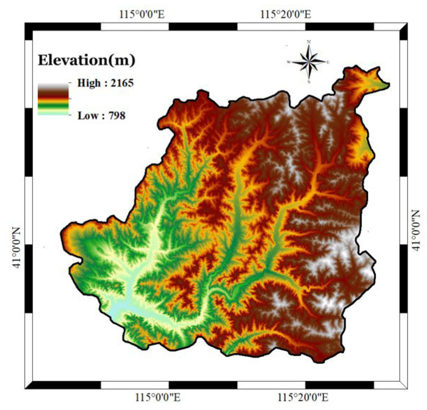
2.1. Overview of the Study Area

The research area is located in Chongli District, Zhangjiakou City, Hebei Province, China, in the northwest of Hebei Province, and the transitional zone between the Inner Mongolia Plateau and North China Plain. The geographical location is between 114 17′–115 34′ E and 40 47′–41 17′ N, as shown in Figure 1. The total area of Chongli District is 2334 square kilometers, of which 80% is mountainous and the forest coverage rate is 52.38%. The terrain in this area is steep, and the landform is mainly Zhongshan, and some of them are low mountains and hills. The elevation extends from 813 m to 2174 m, with a maximum height difference of 1361 m.

The climate belongs to the continental seasonal climate in the mid-temperate and semi-arid areas, and the distribution of the average temperature in the county is greatly influenced by the topography.

The average temperature in summer is 19 °C, and in winter it is −12 °C, and its isotherm is northeast-southwest. In addition, the average wind speed in this area is only grade 2, with early snowfall and a long snow-covered period. The average annual precipitation is 483.3 mm, the total precipitation is 1.13 billion cubic meters, and the total annual runoff is 100.69 million cubic meters.

Chongli District is rich in vegetation resources. The main vegetation types are broad-leaved forest, mixed coniferous forest, deciduous coniferous forest, evergreen coniferous forest, and shrubs. In addition, there are 3867 hectares of artificial forest and 10,220 hectares of forest protection area, and the forest coverage rate reached 67% in 2021. Therefore, it is necessary to predict the occurrence of forest fires in this area.

2.2. Generations of Data Sets

Many factors contribute to the occurrence of forest fires [39], making it critical to quickly identify their geographic and temporal location, scale range, and environmental causes. The accuracy of forest fire forecasts can be affected by the spatial expanse, spatial and temporal scales, and various anthropogenic environmental conditions. Hence, it is crucial to reasonably determine the influential factors in forest fire prediction to improve the model’s accuracy.

2.2.1. Data Source

The two types of data sources chosen in this paper to study the Chongli district are remote sensing data and meteorological data. These sources were chosen concerning the satellite image information and the current records of fire information from previous years. The remote sensing data include geographic factors and vegetation factors. The meteorological information includes information on temperature, wind, rainfall, and other variables.

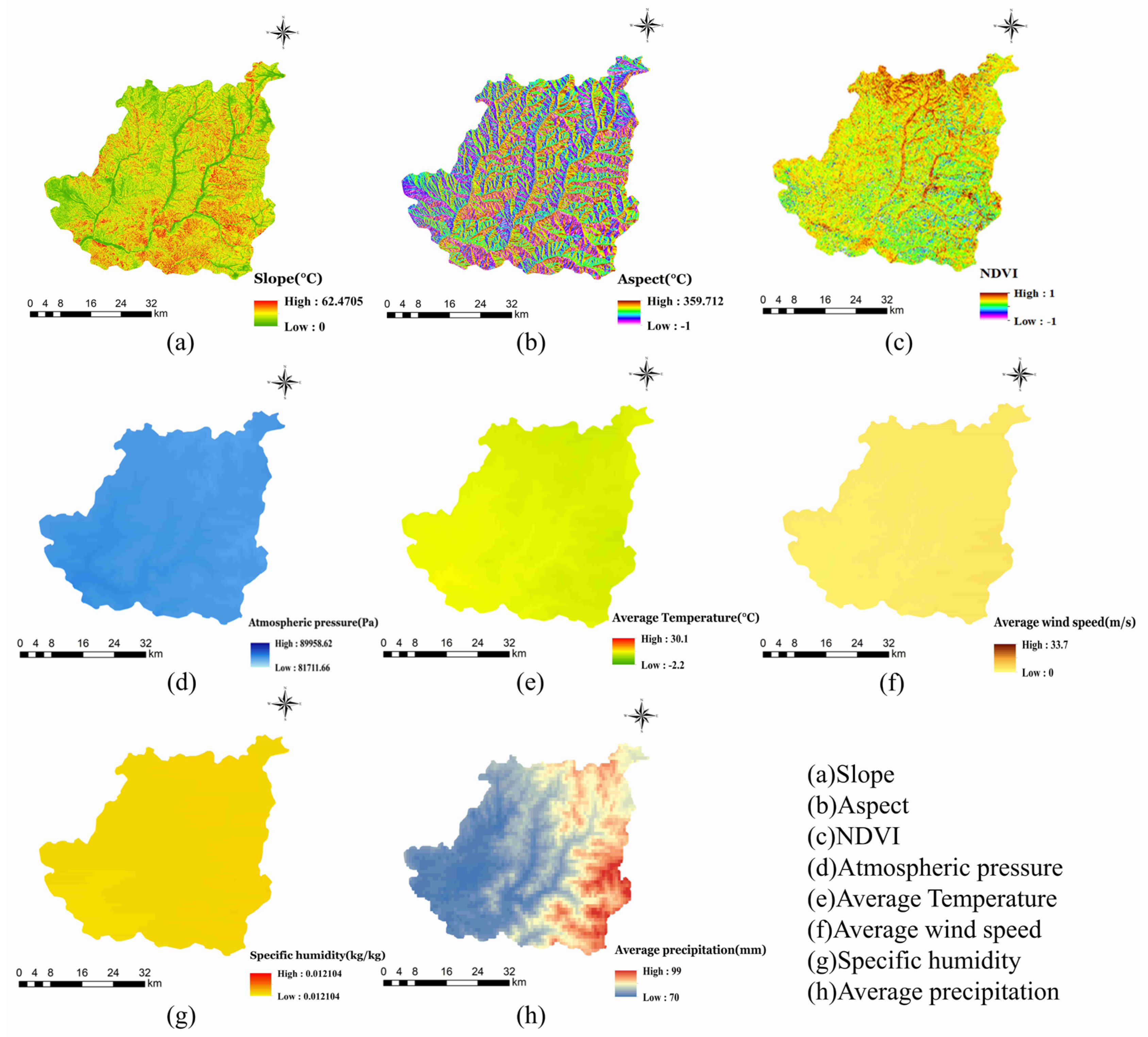
2.2.2. Factors Influencing Forest Fires

In this study, the data from 2020–2021 were chosen as the historical fire data set, during which the Chongli district experienced 22 fires, including 15 fires in the spring, which accounted for 68% of the total number of fires, the majority of which took place in the eastern part of the study area. Based on previous studies [40], and considering various influencing factors such as meteorology and geography [41], eight forest influencing factors were finally identified, as shown in

Table 1. Data description of forest fire influence.

No.	Data	Scale/Resolution Original	Unit	Original Data Format	Source
1	Slope	30 m	m	Raster	ASTER GDEM
2	Aspect	30 m	degree	Raster
3	NDVI	500 m		Raster	Sentinel-2
4	Average temperature	-	°C	NetCDF	CIMISS
5	Average precipitation	-	kg/m2	NetCDF
6	Average wind speed	-	m/s	NetCDF
7	Specific humidity	-	kg/kg	NetCDF
8	Atmospheric pressure	-	Pa	NetCDF

ASTER GDEM: advanced spaceborne thermal emission and reflection radiometer global digital elevation map. Sentinel-2 is a high-resolution multispectral imaging satellite. NetCDF: network common data form. NDVI: normalized difference vegetation index. CIMISS: China Integrated Meteorological Information Service System.

.

In this paper, the forest fire influencing factor maps are shown in Figure 2, where the geographic factors include slope and slope direction. The moisture in the soil is impacted by how steep the slope is. Gravity causes more severe soil erosion in high-slope areas, which leads to dry vegetation and increases the risk of hill fires. There are sunny and shady slopes. Hill fires are more likely to occur in vegetation on sunny slopes due to prolonged exposure to sunlight, an increase in the local temperature, and a decrease in the air’s humidity.

One of the most significant factors influencing the likelihood of forest fires is the weather [33,39,42,43], and many experts and academics have concluded research and analysis that meteorological factors like temperature, wind speed, relative humidity, rainfall, and atmospheric pressure can be used to predict both the risk of forest fires and their occurrence [40,44,45]. The likelihood of a forest fire as well as its changing trend can be reflected by the forest fire risk indicator, which is a crucial tool for anticipating and assessing forest fire situations. In a sense, the accurate prediction of the relevant meteorological factors will enable the accurate prediction of forest fire risk, enabling the more effective deployment of forest fire prevention and control work.

In this paper, the influencing factors of meteorology were obtained from CIMISS, including average temperature, average precipitation, average wind speed, specific humidity, and atmospheric pressure. The topographic data were pre-processed, and the slope and slope direction were extracted from the digital elevation model (DEM). Additionally, Sentinel-2 satellite data was used to extract the normalized vegetation index $NDVI$.

The $NDVI$ has been recognized as a crucial factor in the modeling of forest fires [46]. $NDVI$ is remote sensing data that reflects the spatial distribution of vegetation and vegetation density and is the ratio of the difference between the $NIR$(near infrared reflectance) and red bands and the sum of both, and all NDVI ranges in the interval [−1, 1]. The $NIR$ and red bands of various surface objects have varying values. The satellite’s sensors can calculate the $NDVI$ from these two bands, and the $NDVI$ can also be used to determine surface coverings. The $NDVI$ of water and clouds is typically negative, while that of bare soil and rocks is zero. The higher the vegetation density, the closer the $NDVI$ is to 1. Areas with high $NDVI$ are more likely to cause hill fires under high-temperature conditions or human influence, so $NDVI$ is an important factor influencing hill fires. The following is the $NDVI$ calculation formula.

$$NDVI=\frac{(NIR-Red)}{(NIR+Red)}$$

(1)

2.3. Impact Factor Assessment

To predict forest fires, the features chosen are crucial. The prediction process will become more difficult and seriously impair the model’s accuracy if the chosen influencing factors have an excessively high correlation or linear relationship. Therefore, all data should be examined and analyzed to avoid data distortion caused by interactions between data. In this study, the data are tested using the multicollinearity test and Pearson analysis.

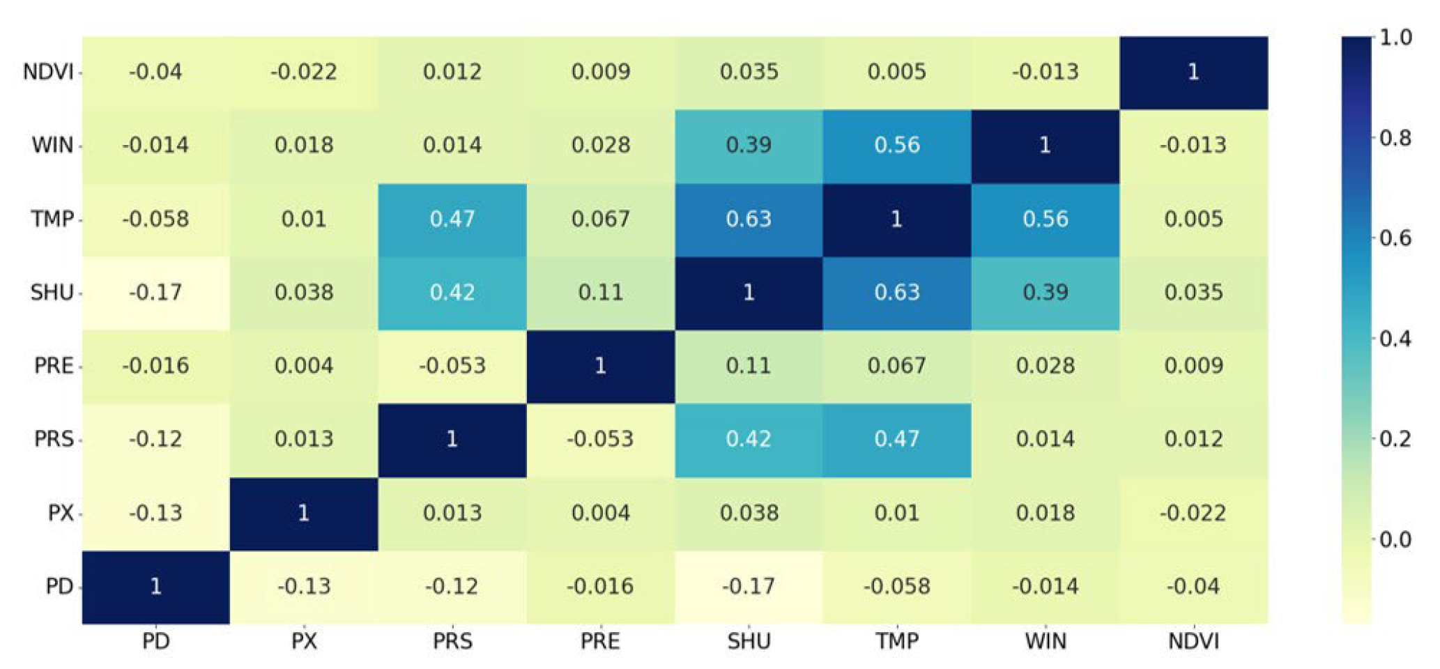
2.3.1. Pearson Analysis

In statistics, the Pearson correlation coefficient, also called Pearson product-moment correlation coefficient, is used to measure the correlation (linear correlation) between two variables X and Y.

In this paper, Pearson analysis is used to analyze the correlation between forest fire impact factors, and the Pearson correlation coefficient is an indicator of the degree of the direct correlation between two variables. In general, two variables have positive, negative, and uncorrelated associations. Pearson correlation coefficient measures the degree of a direct correlation between two variables and is expressed as a value from −1 to 1. Here is a formula for the Pearson correlation coefficient.

$${\rho }_{x,y}=\frac{E(xy)-E(x)E(y)}{\sqrt{E(x^2)-E^2(x)}\sqrt{E(y^2)-E^2(y)}}$$

(2)

The influence factors selected in this paper include slope (PD), slope direction (PX), average precipitation (PRE), atmospheric pressure (PRS), specific humidity (SHU), average temperature (TMP), and average wind speed (WIN). The Pearson correlation coefficients between the factors are shown in Figure 3.

A high degree of correlation exists between two variables when the Pearson correlation coefficient’s absolute value is larger than 0.8. Figure 3 demonstrates that there are no highly connected factors. The largest correlation coefficient is 0.629 for the average temperature and specific humidity.

2.3.2. Multicollinearity Test

Multicollinearity refers to the existence of complete or near-complete linear relationships among the variables in the equation, which can lead to the loss of significance tests and failure of the model prediction function.

In order to further determine whether there is a linear relationship between the forest fire factors and prevent the relationship between the factors from affecting the model prediction inaccuracy, the forest fire influence factors were further tested using the multicollinearity test. To analyze the correlation of the elements that cause forest fires, assessment measures like the $VIF$ variance inflation factor) and $TOL$ (tolerance) are frequently utilized. The following are the calculating methods.

$$VIF=\frac{1}{1-R_i{}^2}$$

(3)

$$TOL=1-R_i{}^2$$

(4)

where $R_i{}^2$ is the goodness of fit of the linear fit between the ith feature and the remaining features. If TOL is less than 0.1 or VIF is greater than 10, the factors are considered to have collinearity, and the test results of each influence factor are shown in

Table 2. Multicollinearity analysis of forest fire influencing factors.

No.	Forest Fire Influencing Factor	TOL	VIF
1	Slope	0.945	1.058
2	Aspect	0.982	1.018
3	NDVI	0.996	1.004
4	Average temperature	0.394	2.536
5	Average precipitation	0.971	1.030
6	Average wind speed	0.592	1.690
7	Specific humidity	0.554	1.804
8	Atmospheric pressure	0.644	1.554

According to the multicollinearity test as shown in Table 2, the VIFs of the eight forest fire influence factors in the table are all less than 10 and the tolerance is greater than 0.1, indicating that there is no multicollinearity among the selected forest fire influence factors, i.e., there is no case of redundant factors, and all of them can be used as the predicted forest fire factors.

. After the test, the VIF of all factors is less than 10, and the features are considered not to have collinearity.

The data source for the study of the Chongli district in this paper consists of two parts, namely, geographic data and meteorological data. To prevent bias from imbalanced factor sizes, eight meteorological and topographical affecting factors were chosen for normalization. We converted the raster into a digital format using the ArcGIS software, and each feature was then converted into a raster with the same pixel size (1000 × 1000 m), data type (8-bit unsigned integer), and coordinate system (GCS WGS 1984). This process produced a total of 2125 rasters. The raster features are then converted into point elements, and the image element value of each raster is obtained and the latitude and longitude are calculated using the GCS_WGS_1984 coordinates, resulting in a dataset with the time stamp and latitude and longitude combined as indexes, the eight influencing factors of meteorology and topography as features, and the occurrence or non-occurrence of fire as labels.

Below is the normalization equation.

$$y=2\times \frac{x-x_{min}}{x_{max}-x_{min}}-1$$

(5)

where x corresponds to each data, y is the normalized result, x_min is the minimum value in that category, and x_max is the maximum value in that category.

Category imbalance in the dataset is a common occurrence in the forest fire prediction problem. Category imbalance means that the number of events in the non-fire category is much larger than the number of events in the fire category, and category imbalance can adversely affect the classification performance of the model. In addition, it has been established that oversampling is a reliable approach to address this issue [47]. According to Waldo Tobler’s first law of geography (the correlation between features is related to distance; generally, the closer the distance, the greater the correlation between features, the farther the distance, the greater the dissimilarity between features) [48], taking into account the spatial aggregation of fires [49], an area close to the fire vector point pixel may also be a fire-prone area.

In this paper, we use buffer analysis and oversampling joint method to increase the number of fire-like events, which reduces the effect of the sample imbalance phenomenon to some extent. At the same time, it also reduces the regional differences in different geographical locations and improves the differences between fire point data and non-fire point data. To start, 20% (88,819) of the 444,096 samples are separated into a test set. The remaining samples are then oversampled to form a 5 km square buffer, with pixels inside the buffer being rescaled to 1 (fire) and those outside being rescaled to 0 (non-fire class). Through the above processing of forest fire data, the forest fire dataset used in this paper was obtained.

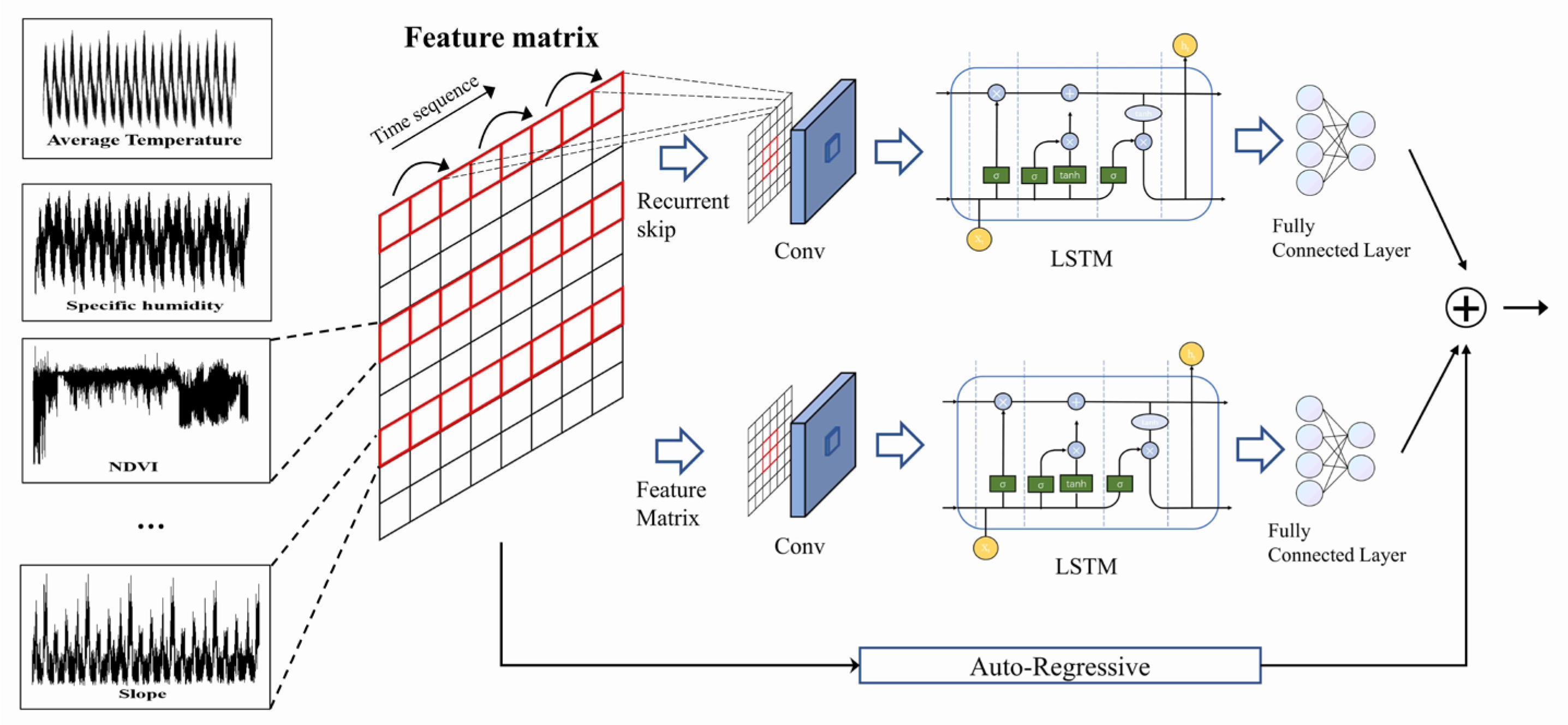
2.4. Algorithm Model

Lai et al. [50] first proposed Long- and Short-term Time-series Network (LSTNet) in 2018. It is a deep learning framework for multivariate time series, and it can effectively use the multidimensional relationship between variables to achieve better prediction results. Based on LSTM recurrent neural network, Weicong Kong et al. [51] realized short-term residential load forecasting. According to the multidimensional information matrix and LSTNet, Zhanlong Zhang et al. [52] proposed a prediction method for the line loss rate of network low-voltage distribution network, and it also showed a good prediction effect.

The LSTNet model consists of a nonlinear part and a linear part. The nonlinear part consists of a convolutional layer, a recurrent layer, and a recurrent-skip layer, which are fused using a fully connected layer to obtain the prediction results, while the linear part uses an autoregressive model to predict the results. The results of the nonlinear part and the linear part are superimposed to obtain the final prediction results. In this paper, a forest fire prediction model based on LSTNet is established, and the overall structure is shown in Figure 4.

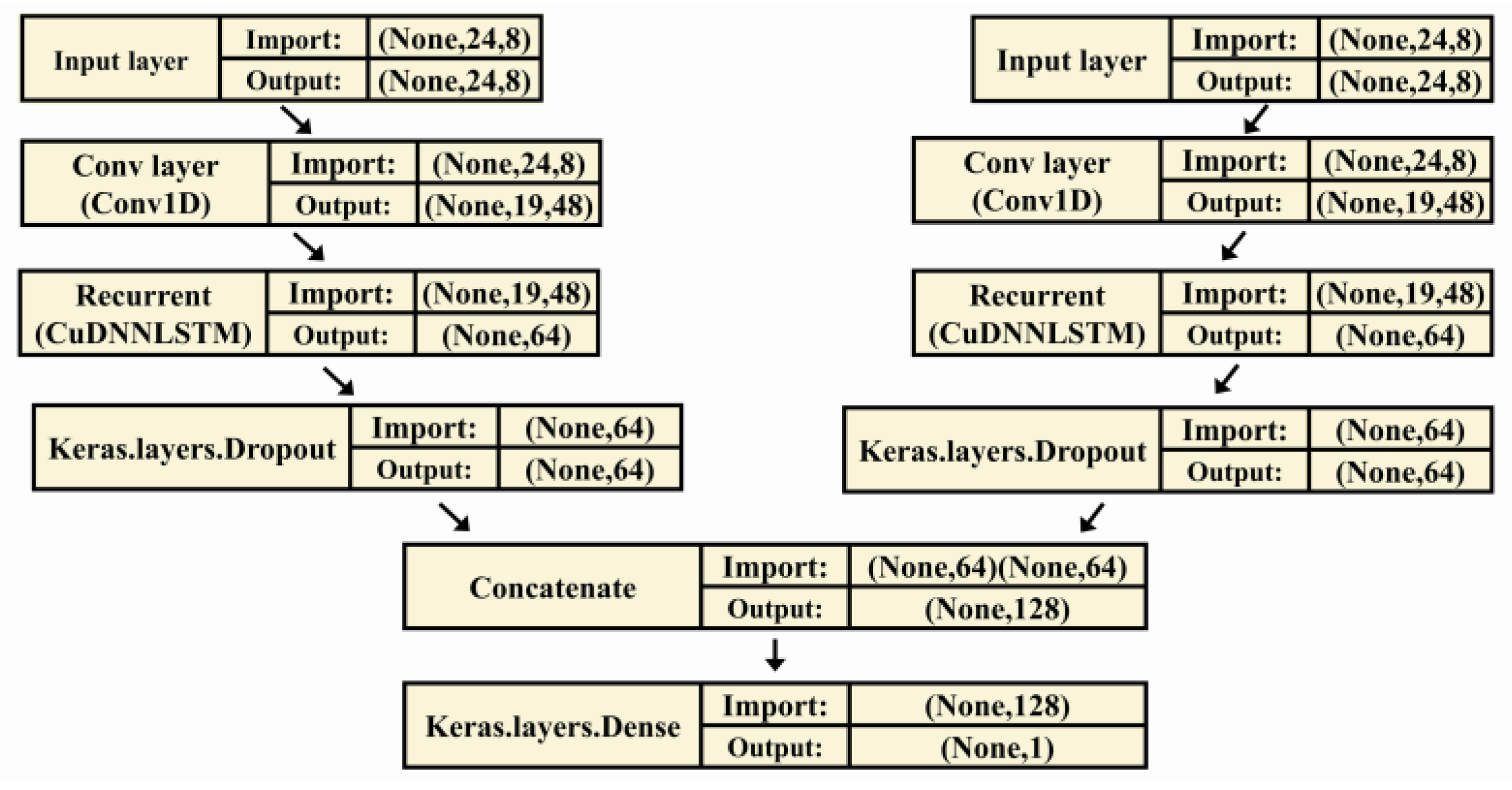
2.4.1. Convolutional Component

CNN (Convolutional Neural Network) is a feed-forward neural network model that is frequently used in the field of deep learning. It is mostly utilized in the field of image recognition due to its high feature learning capabilities and capacity to significantly reduce the number of model parameters. Currently, CNN is frequently used for processing time series. A pooling-free convolutional network serves as the first layer of the LSTNet framework. It slides over the time dimension in which the time series is placed using a convolutional kernel to extract the short-time correlations of the time dimension corresponding to the size of the time series, and to acquire the dependencies between neighboring time series data. The convolution layer consists of multiple filters of width $\omega$ and height n (the height is set to be the same as the number of variables). The $k$th filter sweeps the input matrix $X$ and produces $h_k$.

$$h_k=RELU(W_k\ast X+b_k)$$

(6)

$${\left[C\ast X\right]}_{i,j}={\displaystyle \sum _m^{}{\displaystyle \sum _n^{}{C}_{m,n}\times X_{i+m,j+n}}}$$

(7)

where $\ast$ denotes the convolution operation and the output is a vector, $h_k$ is the output feature vector, $W_k$ is the weight matrix connected to the convolutional kernel of the $k$th feature, the activation function $RELU(x)=max(0,x)$, and $b_k$ is the bias vector of the feature. The left side of the input matrix $X$ is padded with zeros so that each vector $h_k$ is of length $T$. The size of the output matrix of the convolutional layer is $d_c\times T$, where $d_c$ denotes the number of filters.

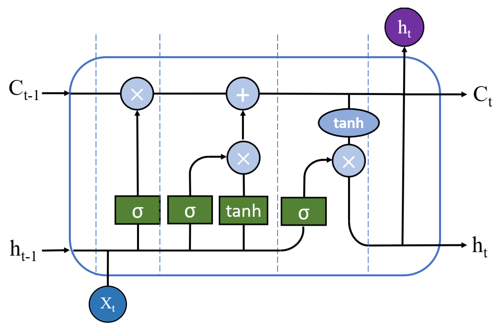
2.4.2. Recurrent Component

RNN (Recurrent Neural Networks) is very effective for data with sequence characteristics. It can mine the time sequence information and semantic information in the data and memorize the previous information and apply it to the calculation of the current output [53]. The recurrent component and the recurrent-skip component receive the output of the convolution layer. To reduce gradient disappearance and achieve association extraction prior to the single-step cycle, this component employs LSTM units. The cell’s structure is illustrated in Figure 5.

$$h_t=(1-u_t)\odot h_{t-1}+u_t\odot c_t$$

(8)

The model structure of the hidden state of the cyclic unit at the time $t$ can be expressed as follows.

$$r_t=\sigma (x_t{W}_{xr}+h_{t-1}{W}_{hr}+b_r)$$

(9)

$$u_t=\sigma (x_t{W}_{xu}+h_{t-1}{W}_{hu}+b_u)$$

(10)

$$c_t=ReLU[x_t{W}_{xc}+r_t\ast (h_{t-1}{W}_{hc})+b_c]$$

(11)

$$h_t=(1-u_t)\ast h_{t-1}+u_t\odot c_t$$

(12)

where $r_t$ is the degree of ignoring the state information of the previous moment, $\sigma$ is the sigmoid function, $x_t$ is the input of the layer at the time of $t$, $\ast$ is the product of elements, $W_{hr}$, $W_{xu}$, $W_{hu}$, $W_{xc}$, $W_{hc}$ are the connection weights between different states, $h_t$ is the hidden state at each time step, $b_r$, $b_u$, $b_c$ are the deviations of different states, and $u_t$ is the degree of influence of the state information of the previous moment in the current state.

2.4.3. Recurrent-Skip Component

The LSTM units of the recurrent layer can memorize historical information and capture long-term dependencies in the sequence. Due to the presence of gradient disappearance, the LSTM cannot capture repetitive patterns in the time series for a considerable period of time, so the temporal dimension of the information flow is extended by adding a recurrent-skip component. The update process is represented as follows.

$$r_t=\sigma (x_t{W}_{xr}+h_{t-p}{W}_{hr}+b_r)$$

(13)

$$u_t=\sigma (x_t{w}_{xu}+h_{t-p}{W}_{hu}+b_u)$$

(14)

$$c_t=RELU[x_t{W}_{xc}+r_t\odot (h_{t-p}{W}_{hc})+b_c]$$

(15)

$$h_t=(1-u_t)\odot h_{t-p}+u_t\odot c_t$$

(16)

where $p$ is the number of hidden cells skipped. Considering the existence of periodic parameters such as temperature, this paper selects $p=24$, and optimizes the other parameters.

The model uses a linear combination of two recurrent network structures, the recurrent component, and the recurrent-skip component, to represent the output. We use $\{h^S{}_{t-p+1},h^S{}_{t-p+2},...,h^S{}_t\}$ to denote the output of the loop layer at time $t$ and $h_t{}^R$ to denote the output of the loop skip layer from time $t-p+1$ to time $t$. We then use a fully connected layer to combine the outputs of the recurrent layer and the recurrent-skip layer as the prediction results of the nonlinear part, which is predicted as follows.

$$h_t{}^D=W^R{h}_t{}^R+{\displaystyle \sum _{i=0}^{p-1}{W}_i{}^S{h}^S{}_{t-i}+b}$$

(17)

where $h_t{}^D$ is the prediction of the nonlinear part at moment t.

2.4.4. Autoregressive Component

Since the convolutional and recurrent layers do not have linear characteristics, this makes the output of the neural network model insensitive to the input data. Moreover, in the real data set, the scale of the input signal is produced to change continuously, which makes the prediction of the network much less effective. Therefore, the autoregressive (AR) model is used to predict the linear part of the load data terminals. The prediction results of the AR layer are as follows.

$$h^L{}_{t,i}={\displaystyle \sum _{k=0}^{q^{\alpha r}-1}{W}_k{}^{\alpha r}{y}_{t-k,i}+b^{\alpha r}}$$

(18)

where $h^L{}_{t,i}$ is the prediction result of the AR model, $q^{\alpha r}$ is the input window size, and $h_t{}^L$ is the prediction result of the linear part. The final results of LSTNet are obtained by integrating the outputs of the neural network part and the AR model.

$$Y_t=h_{\mathrm{t}}{}^D+h_t{}^L$$

(19)

where $Y_t$ denotes the final prediction result at timestamp $t$.

3. Results

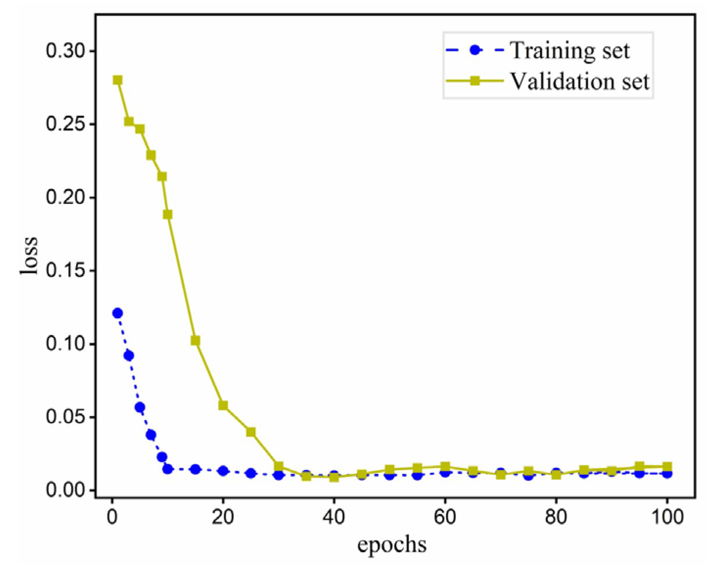
3.1. Model Parameters and Accuracy

The LSTNet model used in this paper has an input dimension of 8 and an output dimension of 1, including 2 inputs, 2 convolutional layers with 1-dimensional depooling layers (Conv1D), 1 recurrent layer, 1 recurrent jump layer, and 1 fully connected layer (Dense). The multi-layer network architecture can be used for deeper data mining with the following parameters: timestep = 24, batch_size = 64, epochs = 100, and the optimizer is ‘Adam’. The parameter structure of the model in this paper is shown in Figure 6. Take the first layer (None, 24, 8) as an example, which denotes the number of samples, time step, and variable dimension respectively.

In this paper, MSE (mean square error) is chosen as the loss function. The LSTNet model’s training loss curve is displayed in Figure 7 after training, from which it can be deduced that the model converges and validation sets converge at 0.01 after roughly 100 iterations of training, demonstrating that the model has favorable performance.

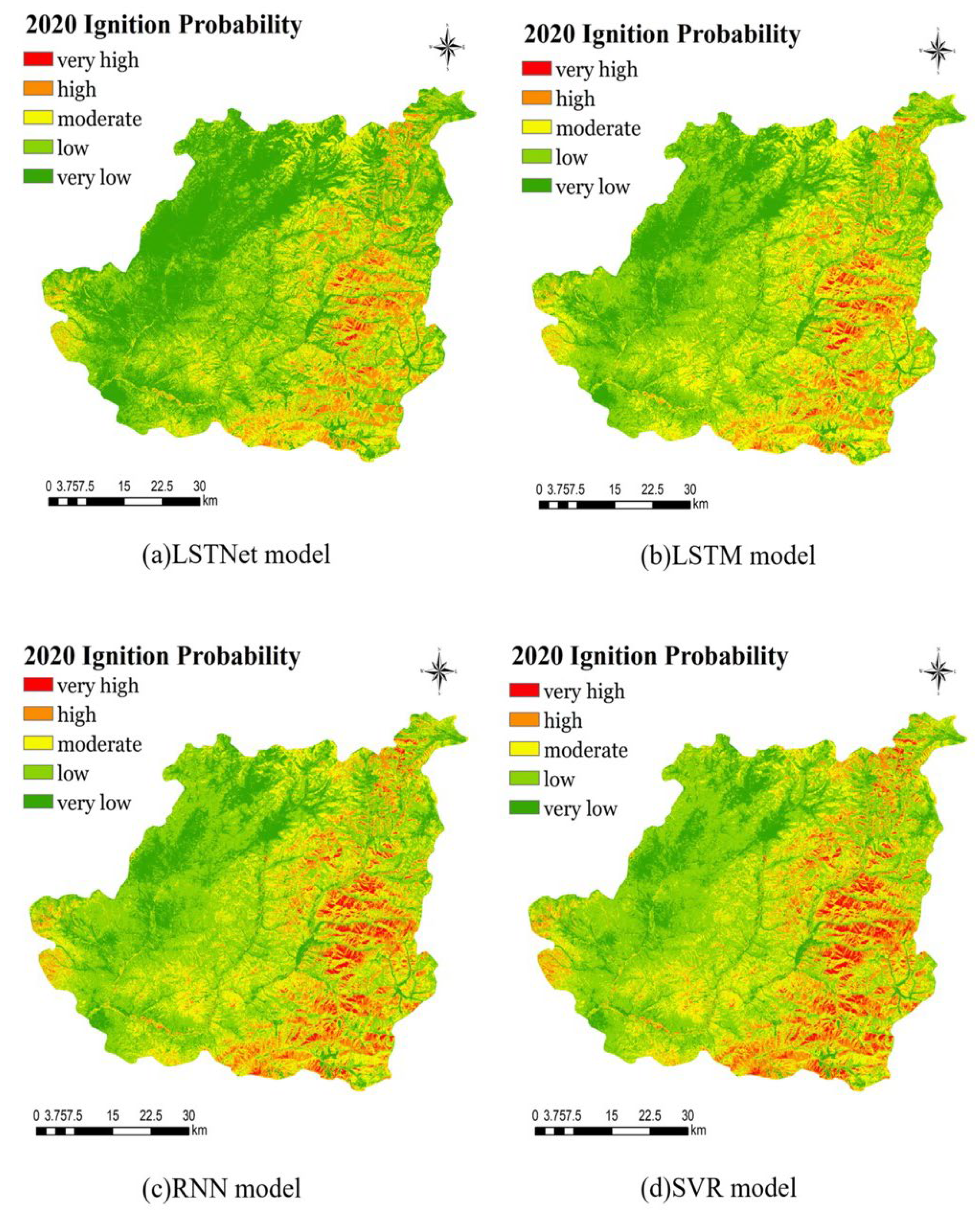
3.2. Forest Fire Susceptibility Mapping

After training, we obtained a classification model, and input the data from the test set into the classification model (LSTNet). We also used a traditional machine learning model such as SVM to predict forest fire susceptibility by inputting data from the test set. In this paper, we used the LSTNet model and ArcGIS to map the forest fire risk prediction results for Chongli in 2020, which are shown in Figure 8 together with the prediction results of other methods.

From the results of the forest fire risk forecast map, we can see that the forest fire risk points in Chongli are mainly located in the eastern and southeastern parts of the country. The northwestern and southwestern areas are the least vulnerable to forest fires. The risk level in the forest fire susceptibility map drawn by LSTNet is relatively uniform, while the traditional model predicts that most of the areas are in the medium to high level. In fact, the vast majority of Chongli is less likely to experience hill fires, while the traditional machine learning model predicts a relatively high risk of forest fires for the entire Chongli area in order to fit the sample, which is where the traditional machine learning model falls short.

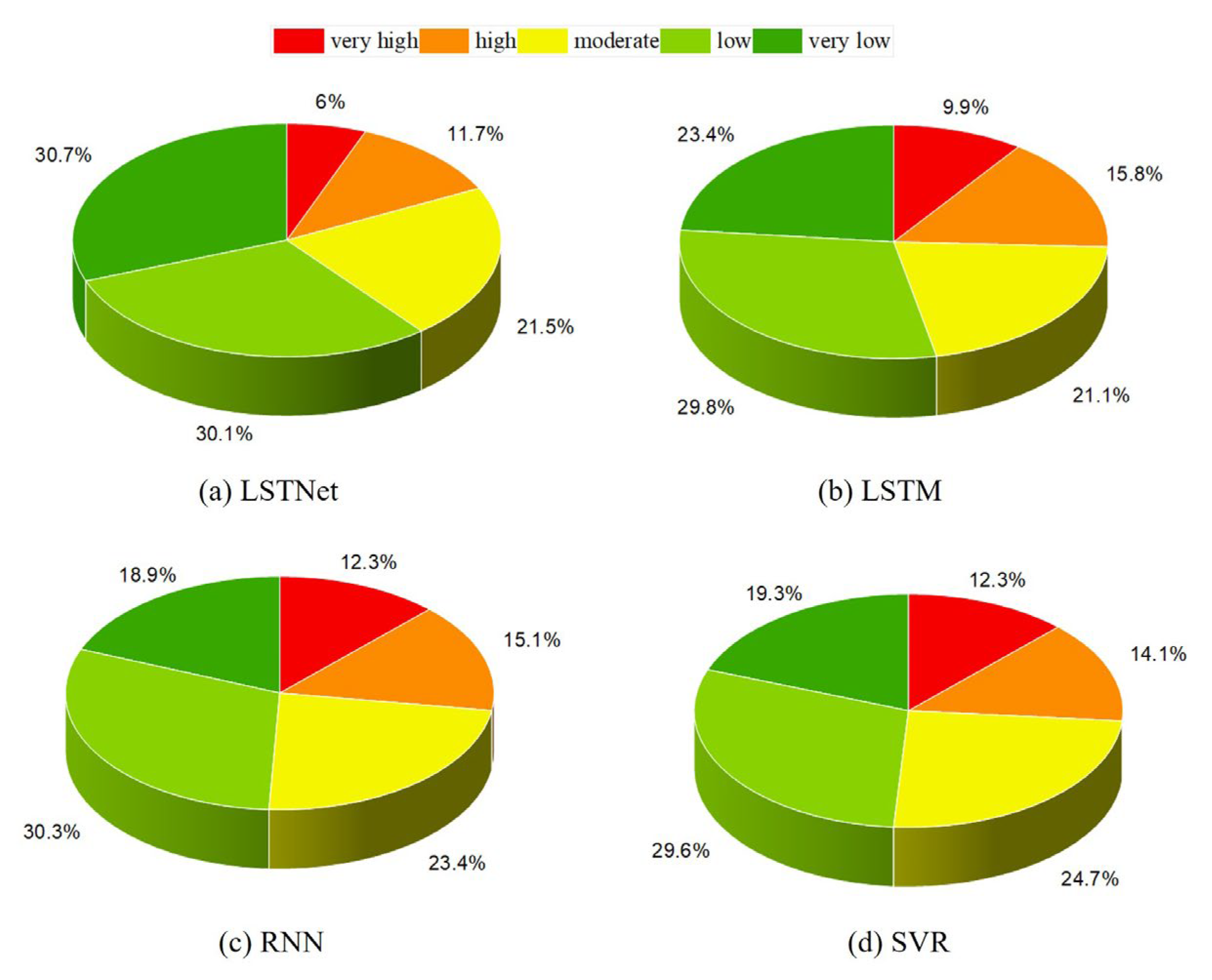
3.3. Predicted Forest Fire Class Distribution of Various Models

Figure 9 shows the proportion of each level of the image element to the total image element in Chongli District. It basically shows that the distribution of forest fire susceptibility in Chongli District is relatively good, and most of the areas are in non-high-risk areas with low risk of a forest fire. For the prediction of high-risk areas, the LSTNet model has 11.7% high, the LSTM model has 15.8% high, the RNN model has 15.1% high, and the SVR model has 14.1% high, which shows that for the prediction of high-risk areas, the prediction results of LSTNet are smaller than other models. At the same time, the LSTNet model has a reasonable division of susceptibility level, and the very low risk area accounts for a large proportion of the whole Chongli district and has the largest difference with the mask of the very high risk area, while the traditional machine learning model cannot effectively divide the very high risk and very low-risk areas, which cannot reflect the bipolar distribution of very high risk and very low risk of mountain fires, and the intermediate level is more vague information for managers. The intermediate level is relatively vague information, which is not conducive for managers to make appropriate decision-making measures.

4. Discussion

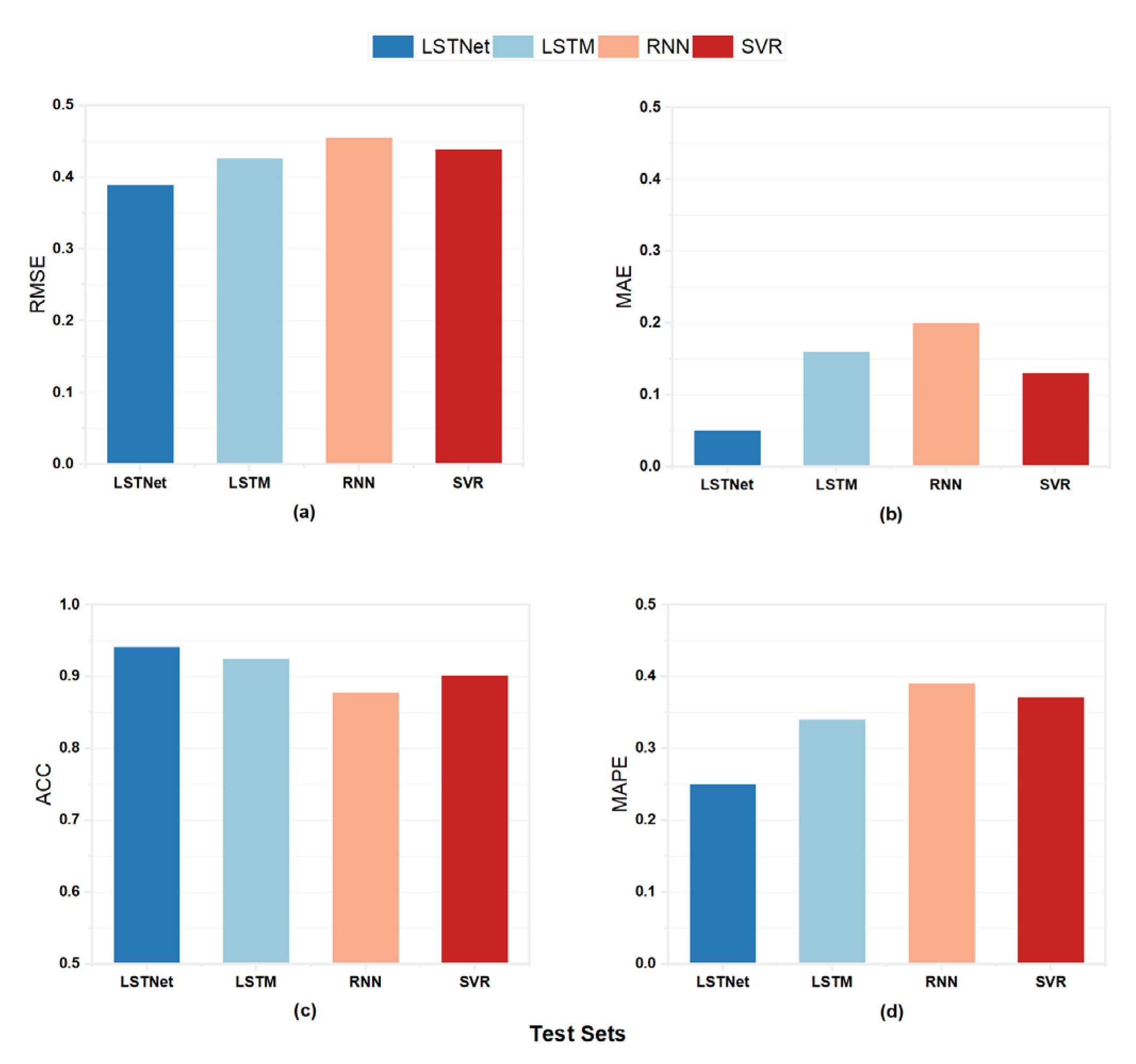
4.1. Model Evaluation Metrics

The forest fire factor consists of meteorological and geographical factors, and considering the existence of certain periodicity and seasonality of the forest fire factor in the time series, this paper uses $RMSE$ (root mean square error), $MAE$ (mean absolute error), $MAPE$ (mean absolute percentage error), and ACC (Accuracy) to evaluate the prediction effect of each model. The formulas for each index are as follows.

$$RMSE=\sqrt{\frac{1}{M}{\displaystyle \sum _{i=1}^M{(y_i-{\widehat{y}}_i)}^2}}$$

(20)

$$MAE=\frac{1}{M}{\displaystyle \sum _{i=1}^M|y_i-{\widehat{y}}_i|}$$

(21)

$$MAPE=\frac{100\%}{n}{\displaystyle \sum _{i=1}^n\left|\frac{{\widehat{y}}_i-y_i}{y_i}\right|}$$

(22)

where $y_i$ is the label of the sample $i$. The positive class of fire points is denoted by 1, and the negative class of non-fire points is denoted by 0.

$$ACC=\frac{(TP+TN)}{(TP+TN+FN+FP)}$$

(23)

where $TP$ (True Positive) is the number of fire points judged as fire points by the model package, $FN$ (False Negative) is the number of fire points judged as non-fire points by the model, $FP$ (False Positive) is the number of non-fire points judged as fire points by the model, and $TN$ (True Negative) is the number of non-fire points judged as non-fire points by the model.

4.2. Model Comparison

In this paper, the four models are compared using RMSE, MAE, ACC, and MAPE metrics, and the comparison results are shown in Figure 10. The overall performance of the LSTNet model is better in the test set, especially in the comparison of the ACC metric of the model reaching the highest value of 0.941. In addition, LSTNet is smaller than other models in the comparison of RMS, MAE, and MAPE metrics. From this, we can see that the deep learning model is better than the traditional machine learning algorithm for forest fire prediction in the face of large amounts of data, and also combined with Figure 8 and Figure 9, we can see that the model is better reflecting the spatial distribution of forest fire risk and effectively dividing the very high risk and very low risk zones. It is worth noting that LSTNet is a variant of LSTM, so the values of RMSE and ACC are closer between the two models in Figure 10, which also shows that the LSTM model has higher accuracy in multivariate spatiotemporal prediction problems, which echoes the previously mentioned literature [33,35,37,38]. Recurrent-skip layer makes it perform better in MSE and MAPE. In summary, the prediction results of the LSTNet model are more obvious in spatial pattern, reflecting the bipolar distribution of the very high and very low risk of mountain fires, which can distinguish high and low risk areas more clearly, tap the spatial background information, and improve the accuracy of classification.

5. Conclusions

In view of the spatial and temporal characteristics of forest fires and the short-term dependence and long-term repeatability among forest fire factors, this paper proposes an LSTNet-based forest fire prediction model for spatial prediction of forest fire susceptibility in the Chongli district. Pearson analysis and the multicollinearity test are used to filter and validate the forest fire factors. At the same time, processing methods such as buffer extraction, oversampling, and normalization were designed to improve the prediction accuracy. Because of the uncertainty and periodicity of multivariate forest fire factors, and considering that meteorological factors have long-term and ultra-long-term repetitive patterns, this paper uses the LSTNet model to divide forest fire prediction into linear and nonlinear parts and uses the recurrent-skip layer to capture the features of ultra-long-term period variation. We debugged and optimized the hyperparameters to improve the accuracy of the prediction. The experimental data were input into the trained model, and the forest fire probability prediction map of Chongli district was also drawn with the help of ArcGIS. Finally, ACC, RMSE, and other metrics were used to compare with traditional machine learning methods.

Through the research in this paper, we found that the LSTNet model has higher accuracy and stronger robustness compared with other traditional machine learning models. The results predicted by LSTNet can clearly distinguish between very high and very low sensitive areas, and are more sensitive to spatial pattern information, which can better classify forest fire susceptible areas and reflect a strong generalization ability. In conclusion, LSTNet can effectively extract neighborhood information, grasp the periodic change characteristics of forest fire factors, achieve efficient feature extraction, and then improve classification accuracy. This study has some reference value for forest fire planning and forest fire avoidance but still has some limitations, and the influence of other forest fire factor variables on forest fire prediction has not been studied in depth. This paper also shows that the model has a good prediction effect on multivariate prediction problems and can also be used for prediction studies in other fields such as photovoltaic and wind power.

References

1. Hao-ruo, Y. Studies on Controlling Strategy for Forest Fire under the Global Warm Climate. 2009. Available online: https://typeset.io/papers/studies-on-controlling-strategy-for-forest-fire-under-the-pf9obfpr6x (accessed on 6 March 2023).
2. Pechony, O.; Shindell, D.T. Driving forces of global wildfires over the past millennium and the forthcoming century. Proc. Natl. Acad. Sci. USA 2010, 107, 19167–19170. [Google Scholar] [CrossRef] [Green Version]
3. Cisneros, R.; Schweizer, D.W.; Tarnay, L.; Navarro, K.M.; Veloz, D.; Procter, C.T. Climate Change, Forest Fires, and Health in California. In Climate Change and Air Pollution; Springer: Cham, Switzerland, 2018. [Google Scholar]
4. Zhang, Y.; Qin, D.; Yuan, W.; Jia, B. Historical trends of forest fires and carbon emissions in China from 1988 to 2012. J. Geophys. Res. Biogeosci. 2016, 121, 2506–2517. [Google Scholar] [CrossRef]
5. Mahalingam, S.; Deep, M.S.; Krishna, K.S. Wireless Sensor Based Forest Fire Early Detection with Online Remote Monitoring. Int. J. Eng. Adv. Technol. 2021, 10, 143–145. [Google Scholar] [CrossRef]
6. Fried, J.S.; Gilless, J.K.; Riley, W.J.; Moody, T.J.; Simón de Blas, C.; Hayhoe, K.; Moritz, M.A.; Stephens, S.L.; Torn, M.S. Predicting the effect of climate change on wildfire behavior and initial attack success. Clim. Change 2008, 87, 251–264. [Google Scholar] [CrossRef] [Green Version]
7. Fried, J.S.; Torn, M.S.; Mills, E. The Impact of Climate Change on Wildfire Severity: A Regional Forecast for Northern California. Clim. Change 2004, 64, 169–191. [Google Scholar] [CrossRef]
8. Baranovskiy, N.V.; Podorovskiy, A.; Malinin, A. Parallel Implementation of the Algorithm to Compute Forest Fire Impact on Infrastructure Facilities of JSC Russian Railways. Algorithms 2021, 14, 333. [Google Scholar] [CrossRef]
9. Barmpoutis, P.; Papaioannou, P.; Dimitropoulos, K.; Grammalidis, N. A Review on Early Forest Fire Detection Systems Using Optical Remote Sensing. Sensors 2020, 20, 6442. [Google Scholar] [CrossRef] [PubMed]
10. Sakr, G.E.; Elhajj, I.H.; Mitri, G.H. Efficient forest fire occurrence prediction for developing countries using two weather parameters. Eng. Appl. Artif. Intell. 2011, 24, 888–894. [Google Scholar] [CrossRef]
11. Pradeep, G.S.; Prasad, M.K.; Kuriakose, S.L.; Ajin, R.S.; Oniga, V.E.; Rajaneesh, A.; Mammen, P.C.; Patel, N.; Nikhil, S.; Danumah, J.H. Forest Fire Risk Zone Mapping of Eravikulam National Park in India. Croat. J. For. Eng. 2021, 43, 199–217. [Google Scholar] [CrossRef]
12. Bowman, D.; Williamson, G.J. River Flows Are a Reliable Index of Forest Fire Risk in the Temperate Tasmanian Wilderness World Heritage Area, Australia. Fire 2021, 4, 22. [Google Scholar] [CrossRef]
13. Gülçin, D.; Deniz, B. Remote sensing and GIS-based forest fire risk zone mapping: The case of Manisa, Turkey. Turk. J. For./Türkiye Orman. Derg. 2020, 21, 15–24. [Google Scholar] [CrossRef] [Green Version]
14. Maffei, C.; Lindenbergh, R.C.; Menenti, M. Combining multi-spectral and thermal remote sensing to predict forest fire characteristics. ISPRS J. Photogramm. Remote Sens. 2021, 181, 400–412. [Google Scholar] [CrossRef]
15. Jin, R.-X.; Lee, K.S. Investigation of Forest Fire Characteristics in North Korea Using Remote Sensing Data and GIS. Remote Sens. 2022, 14, 5836. [Google Scholar] [CrossRef]
16. Tian, Y.; Wu, Z.; Li, M.; Wang, B.; Zhang, X. Forest Fire Spread Monitoring and Vegetation Dynamics Detection Based on Multi-Source Remote Sensing Images. Remote Sens. 2022, 14, 4431. [Google Scholar] [CrossRef]
17. Cunningham, A.A.; Martell, D.L. A Stochastic Model for the Occurrence of Man-caused Forest Fires. Can. J. For. Res. 1973, 3, 282–287. [Google Scholar] [CrossRef]
18. Shi, S.; Yao, C.; Wang, S.; Han, W. A Model Design for Risk Assessment of Line Tripping Caused by Wildfires. Sensors 2018, 18, 1941. [Google Scholar] [CrossRef] [Green Version]
19. Kalantar, B.; Ueda, N.; Idrees, M.O.; Janizadeh, S.; Ahmadi, K.; Shabani, F. Forest Fire Susceptibility Prediction Based on Machine Learning Models with Resampling Algorithms on Remote Sensing Data. Remote Sens. 2020, 12, 3682. [Google Scholar] [CrossRef]
20. Ye, Q.; Huang, P.; Zhang, Z.; Zheng, Y.; Fu, L.; Yang, W. Multiview Learning With Robust Double-Sided Twin SVM. IEEE Trans. Cybern. 2021, 52, 12745–12758. [Google Scholar] [CrossRef]
21. Dampage, U.; Bandaranayake, L.; Wanasinghe, R.; Kottahachchi, K.; Jayasanka, B. Forest fire detection system using wireless sensor networks and machine learning. Sci. Rep. 2021, 12, 46. [Google Scholar] [CrossRef]
22. Qiu, J.; Wang, H.; Shen, W.; Zhang, Y.; Su, H.; Li, M. Quantifying Forest Fire and Post-Fire Vegetation Recovery in the Daxin’anling Area of Northeastern China Using Landsat Time-Series Data and Machine Learning. Remote Sens. 2021, 13, 792. [Google Scholar] [CrossRef]
23. Xu, R.; Lin, H.X.; Lu, K.; Cao, L.; Liu, Y. A Forest Fire Detection System Based on Ensemble Learning. Forests 2021, 12, 217. [Google Scholar] [CrossRef]
24. Bui, D.T.; Le, K.; Nguyen, V.C.; Le, H.D.; Revhaug, I. Tropical Forest Fire Susceptibility Mapping at the Cat Ba National Park Area, Hai Phong City, Vietnam, Using GIS-Based Kernel Logistic Regression. Remote Sens. 2016, 8, 347. [Google Scholar]
25. Chang, Y.; Zhu, Z.; Bu, R.; Chen, H.; Feng, Y.-t.; Li, Y.; Hu, Y.; Wang, Z. Predicting fire occurrence patterns with logistic regression in Heilongjiang Province, China. Landsc. Ecol. 2013, 28, 1989–2004. [Google Scholar] [CrossRef]
26. Bisquert, M.; Caselles, E.; Sánchez, J.M.; Caselles, V. Application of artificial neural networks and logistic regression to the prediction of forest fire danger in Galicia using MODIS data. Int. J. Wildland Fire 2012, 21, 1025–1029. [Google Scholar] [CrossRef]
27. Oliveira, S.; Oehler, F.; San-Miguel-Ayanz, J.; Camia, A. Modeling spatial patterns of fire occurrence in Mediterranean Europe using Multiple Regression and Random Forest. For. Ecol. Manag. 2012, 275, 117–129. [Google Scholar] [CrossRef]
28. Satir, O.; Berberoglu, S.; Donmez, C. Mapping regional forest fire probability using artificial neural network model in a Mediterranean forest ecosystem. Geomat. Nat. Hazards Risk 2016, 7, 1645–1658. [Google Scholar] [CrossRef] [Green Version]
29. Fan, R.; Pei, M. Lightweight Forest Fire Detection Based on Deep Learning. In Proceedings of the 2021 IEEE 31st International Workshop on Machine Learning for Signal Processing (MLSP), Gold Coast, QLD, Australia, 25–28 October 2021; pp. 1–6. [Google Scholar]
30. Sathishkumar, V.E.; Cho, J.; Subramanian, M.; Naren, O.S. Forest fire and smoke detection using deep learning-based learning without forgetting. Fire Ecol. 2023, 19, 9. [Google Scholar] [CrossRef]
31. Bui, D.T.; Bui, Q.-T.; Nguyen, Q.-P.; Pradhan, B.; Nampak, H.; Trinh, P.T. A hybrid artificial intelligence approach using GIS-based neural-fuzzy inference system and particle swarm optimization for forest fire susceptibility modeling at a tropical area. Agric. For. Meteorol. 2017, 233, 32–44. [Google Scholar]
32. Kang, Y.; Jang, E.; Im, J.; Kwon, C.G. A deep learning model using geostationary satellite data for forest fire detection with reduced detection latency. GISci. Remote Sens. 2022, 59, 2019–2035. [Google Scholar] [CrossRef]
33. Guo, F.t.; Hu, H.q.; Ma, Z.H.; Zhang, Y. Applicability of different models in simulating the relationships between forest fire occurrence and weather factors in Daxing’an Mountains. J. Appl. Ecol. 2010, 21, 159–164. [Google Scholar]
34. Fu, L.; Zhang, D.; Ye, Q. Recurrent Thrifty Attention Network for Remote Sensing Scene Recognition. IEEE Trans. Geosci. Remote Sens. 2020, 59, 8257–8268. [Google Scholar] [CrossRef]
35. Mohajane, M.; Costache, R.; Karimi, F.; Pham, Q.B.; Essahlaoui, A.; Nguyen, H.; Laneve, G.; Oudija, F. Application of remote sensing and machine learning algorithms for forest fire mapping in a Mediterranean area. Ecol. Indic. 2021, 129, 107869. [Google Scholar] [CrossRef]
36. Guo, F.; Zhang, L.; Jin, S.; Tigabu, M.; Su, Z.; Wang, W. Modeling Anthropogenic Fire Occurrence in the Boreal Forest of China Using Logistic Regression and Random Forests. Forests 2016, 7, 250. [Google Scholar] [CrossRef] [Green Version]
37. Natekar, S.; Patil, S.; Nair, A.; Roychowdhury, S. Forest Fire Prediction using LSTM. In Proceedings of the 2021 2nd International Conference for Emerging Technology (INCET), Belgaum, India, 21–23 May 2021; pp. 1–5. [Google Scholar]
38. Murali Mohan, K.V.; Satish, A.R.; Mallikharjuna Rao, K.; Yarava, R.K.; Babu, G.C. Leveraging Machine Learning to Predict Wild Fires. In Proceedings of the 2021 2nd International Conference on Smart Electronics and Communication (ICOSEC), Trichy, India, 7–9 October 2021; pp. 1393–1400. [Google Scholar]
39. Jiang, K.; Chen, L.; Wang, X.; An, F.; Zhang, H.; Yun, T. Simulation on Different Patterns of Mobile Laser Scanning with Extended Application on Solar Beam Illumination for Forest Plot. Forests 2022, 13, 2139. [Google Scholar] [CrossRef]
40. Fu, J.J.; Wu, Z.W.; Yan, S.J.; Zhang, Y.; Gu, X.; Du, L. Effects of climate, vegetation, and topography on spatial patterns of burn severity in the Great Xing’an Mountains. Acta Ecol. Sin. 2020, 40, 1672–1682. [Google Scholar]
41. Li, W.; Xu, Q.; Yi, J.-h.; Liu, J. Predictive model of spatial scale of forest fire driving factors: A case study of Yunnan Province, China. Sci. Rep. 2022, 12, 19029. [Google Scholar] [CrossRef] [PubMed]
42. Guo, F.; Wang, G.; Su, Z.; Liang, H.; Wenhui, W.; Lin, F.; Liu, A. What drives forest fire in Fujian, China? Evidence from logistic regression and Random Forests. Int. J. Wildland Fire 2016, 25, 505–519. [Google Scholar] [CrossRef]
43. Ma, W.; Feng, Z.; Cheng, Z.; Chen, S.; Wang, F. Identifying Forest Fire Driving Factors and Related Impacts in China Using Random Forest Algorithm. Forests 2020, 11, 507. [Google Scholar] [CrossRef]
44. Sharma, K.M.; Thapa, G.B. Analysis and interpretation of forest fire data of Sikkim. For. Soc. 2021, 5, 261–276. [Google Scholar] [CrossRef]
45. Zhu, Y.; Li, D.; Fan, J.; Zhang, H.; Eichhorn, M.P.; Wang, X.; Yun, T. A reinterpretation of the gap fraction of tree crowns from the perspectives of computer graphics and porous media theory. Front. Plant Sci. 2023, 14, 115. [Google Scholar] [CrossRef]
46. Bajocco, S.; Dragoz, E.; Gitas, I.Z.; Smiraglia, D.; Salvati, L.; Ricotta, C. Mapping Forest Fuels through Vegetation Phenology: The Role of Coarse-Resolution Satellite Time-Series. PLoS ONE 2015, 10, e0119811. [Google Scholar] [CrossRef] [PubMed] [Green Version]
47. Schulte, L.A.; Mladenoff, D.J. Severe Wind and Fire Regimes in Northern Forests: Historical Variability at the Regional Scale. Ecology 2005, 86, 431–445. [Google Scholar] [CrossRef]
48. Tobler, W. A Computer Movie Simulating Urban Growth in the Detroit Region. Econ. Geogr. 1970, 46, 234–240. [Google Scholar] [CrossRef]
49. Liang, H.; Zhang, M.; Wang, H. A Neural Network Model for Wildfire Scale Prediction Using Meteorological Factors. IEEE Access 2019, 7, 176746–176755. [Google Scholar] [CrossRef]
50. Lai, G.; Chang, W.-C.; Yang, Y.; Liu, H. Modeling Long- and Short-Term Temporal Patterns with Deep Neural Networks. In Proceedings of the 41st International ACM SIGIR Conference on Research & Development in Information Retrieval, Ann Arbor, MI, USA, 8–12 July 2017. [Google Scholar]
51. Kong, W.; Dong, Z.Y.; Jia, Y.; Hill, D.J.; Xu, Y.; Zhang, Y. Short-Term Residential Load Forecasting Based on LSTM Recurrent Neural Network. IEEE Trans. Smart Grid 2019, 10, 841–851. [Google Scholar] [CrossRef]
52. Zhang, Z.; Yang, Y.; Zhao, H.; Xiao, R. Prediction method of line loss rate in low-voltage distribution network based on multi-dimensional information matrix and dimensional attention mechanism-long-and short-term time-series network. IET Gener. Transm. Distrib. 2022, 16, 4187–4203. [Google Scholar] [CrossRef]
53. Zaremba, W.; Sutskever, I.; Vinyals, O. Recurrent Neural Network Regularization. arXiv 2014, arXiv:1409.2329. [Google Scholar]
Figure 1. Chongli district, Zhangjiakou City, Hebei Province, China.
Forests 14 00778 g001
Figure 2. Forest fire influencing factor maps in 2020 for Chongli district, ZhangjiakouCity, Hebei Province, China.
Forests 14 00778 g002
Figure 3. Heatmap.
Forests 14 00778 g003
Figure 4. The structure of the LSTNet. LSTNet is a long- and short-term time-series network.
Forests 14 00778 g004
Figure 5. Long short-term memory (LSTM).
Forests 14 00778 g005
Figure 6. LSTNet network architecture.
Forests 14 00778 g006
Figure 7. Loss curve.
Forests 14 00778 g007
Figure 8. Premonition map of forest fire risk in Chongli District.
Forests 14 00778 g008
Figure 9. Grade distribution of risk maps predicted by four models.
Forests 14 00778 g009
Figure 10. Model comparison.
Forests 14 00778 g010