TSBA-YOLO: An Improved Tea Diseases Detection Model Based on Attention Mechanisms and Feature Fusion

Abstract

Tea diseases have a significant impact on the yield and quality of tea during the growth of tea trees. The shape and scale of tea diseases are variable, and the tea disease targets are usually small, with the intelligent detection processes of tea diseases also easily disturbed by the complex background of the growing region. In addition, some tea diseases are concentrated in the entire area of the leaves, needing to be inferred from global information. Common target detection models are difficult to solve these problems. Therefore, we proposed an improved tea disease detection model called TSBA-YOLO. We use the dataset of tea diseases collected at the Maoshan Tea Factory in China. The self-attention mechanism was used to enhance the ability of the model to obtain global information on tea diseases. The BiFPN feature fusion network and adaptively spatial feature fusion (ASFF) technology were used to improve the multiscale feature fusion of tea diseases and enhance the ability of the model to resist complex background interference. We integrated the Shuffle Attention mechanism to solve the problem of difficult identifications of small-target tea diseases. In addition, we used data-enhancement methods and transfer learning to expand the dataset and relocate the parameters learned from other plant disease datasets to enhance tea diseases detection. Finally, SIoU was used to further improve the accuracy of the regression. The experimental results show that the proposed model is good at solving a series of problems encountered in the intelligent recognition of tea diseases. The detection accuracy is ahead of the mainstream target detection models, and the detection speed reaches the real-time level.

1. Introduction

China has the largest tea tree plantation area in the world and is also the largest tea-producing country in the world. According to the statistics of the International Tea Commission, the global tea output in 2020 was 6.269 million tons, of which China’s tea output was as high as 2.986 million tons, accounting for 47.6% of the world’s total tea output. In the process of tea planting and growth, tea diseases (including diseases and insect pests) are important factors affecting yield and quality, and serious tea diseases can result in huge economic losses. For example, Anxi County is the largest Oolong tea-producing area in China, with a total tea garden area of 600,000 mu, and suffers economic losses of up to CNY 60 million each year due to tea diseases. The common tea diseases mainly include tea leaf blight, Apolygus lucorum, and tea algae spot. The above-mentioned tea diseases are also the common diseases that cause the greatest harm to the tea tree and can repeatedly infect the tea tree more than once a year. Most of them occur in warm and humid seasons. After the tea plant is infected with the disease, it is often accompanied by the early fall of tea leaves and the withering of the shoots, which leads to a decline in the whole tea plant and even the overall disease of the tea garden, presenting a declining phenomenon, which brings great losses to the majority of tea farmers. When the tea plant becomes infected with the disease, it is necessary to remove the diseased branches or spray pesticides at the early stage of the disease. The conventional wisdom in identifying tea diseases relies heavily on human expertise and inspection (e.g., on-site observation and diagnosis). However, there are various tea diseases with a wide occurrence area, and the manual detection method has strong subjectivity, poor consistency, and a high error rate.

With the rapid development of machine learning, image processing and machine learning are widely applied to recognizing crop diseases. Billah et al. [1] used an adaptive neurofuzzy inference system and color wavelet features for tea disease recognition. Karmokar et al. [2] utilized artificial neural networks (ANNs) to improve the recognition accuracy of tea leaf diseases. A random forest classifier was improved by Chaudhary et al. [3] to classify peanut diseases by combining an attribute evaluation method and the instance filter. Mohan et al. [4] designed an image-processing system for rice leaf diseases using the Haar and AdaBoost classifiers [5] for recognition, with a recognition accuracy of 83.33%. In addition, they also used K-nearest neighbor [6] and support vector machines (SVMs) to classify rice leaf diseases and obtained 91% and 93% accuracy, respectively. Pranjali B. Padol et al. [7] used SVM classifiers to detect grape leaf diseases. After k-means clustering [8], they used SVMs for feature extraction and classification and obtained 85% accuracy. Sun et al. [9] combined SVMs with linear iterative clustering to extract tea disease maps from a complex background, which contributed to the further identification of tea diseases. Adeel et al. [10] segmented and identified grape leaf diseases. During feature extraction, local contrast haze reduction and enhancement techniques were used to improve the image quality. During feature fusion, the neighborhood component analysis method was used to remove redundant features. Based on the experiments, the segmentation and classification accuracy of grape leaf diseases was 90% and 92%, respectively. However, traditional machine learning methods require a large number of images for disease feature extraction, and feature extraction depends on manual design rather than automatic learning.

Spurred by the recent developments in deep learning (DL), many DL-based methods (e.g., CNNs) have been applied to image recognition [11,12,13,14,15,16]. Deep CNNs have more layers and complex structures, meaning they have powerful learning abilities and can automatically extract image features without human expertise and empirical knowledge, resulting in higher recognition accuracy than traditional approaches. Currently, deep CNNs have become the mainstream method in crop disease recognition. Sun et al. [17] used AlexNet to classify tea diseases. They also segmented and enhanced the images of small sample disease datasets and fine-tuned the model parameters during network training. This method obtained better classification results compared with traditional machine learning methods. Zhang et al. [18] used the improved GoogLeNet and Cifar10 to classify and identify maize disease leaves, and both models achieved 98.8% accuracy. Zhong et al. [19] used DenseNet-121 to identify apple leaf diseases and obtained 93.51% accuracy. Agarwal. et al. [20] classified and recognized cucumber leaf diseases. The neural network model was composed of three convolution layers, and a modified activation function was utilized, resulting in a classification accuracy of 93.75%. Hu et al. [21] considered a random combination of U-Net network and full connection conditions to segment and recognize tea diseases, which reduced the interference of the complex background. In conclusion, deep neural networks outperform traditional machine learning methods for disease detection if sufficient datasets are available for training. However, crop disease images are hard to collect, and most of them are of poor quality. In addition, current research on plant disease identification mainly focuses on fruits and food crops, and scant studies exist on utilizing deep learning in detecting tea diseases.

Although CNNs have shown their advantages in detecting tea diseases and other plant diseases, they can suffer from a limited perception field. Due to the mechanism of convolutional computation, the image features extracted by CNNs are constrained to local areas. The limitation of convolution operation makes CNNs lack a global view of the whole-image remote dependencies; these are of great importance for CNNs to focus on (regions of interest) and ignore noise throughout the feature map [22]. In order to address this issue, we propose TSBA-YOLO, a DL tea disease detection model, by making a series of improvements based on YOLOv5 [23], one of the best CNN-based object detectors in recent years. First, the Transformer’s self-attention [24] mechanism is integrated into the convolution layers of the feature extraction network in YOLOv5 as a complementary system. The self-attention mechanism provides our model with a global perception field, which can obtain more contextual information. In addition, we used BIFPN [25] to improve the multiscale feature fusion of tea diseases and enhance the robustness of the tea disease features. Secondly, the Shuffle Attention [26] mechanism is integrated into YOLO’s neck. The use of the Shuffle Attention mechanism enables TSBA-YOLO to pay more attention to tea diseases. The integrated adaptive spatial feature fusion (ASFF) [27] detection head allows the model to automatically filter useless information to suppress the interference of complex backgrounds for tea disease detection. Since the original loss function (i.e., CIoU) of YOLOv5 does not consider the matching of the directions between the prediction box and the target box, this leads to slow convergence. We used SIoU [28] instead of CIoU, the original loss function of YOLOv5, to speed up the convergence of the network and further improve the regression accuracy. Considering the similarity between the characteristics of tea diseases and other plant diseases, a transfer learning strategy was adopted. The model was pretrained by using a public dataset of plant diseases datasets, and then the pretrained model was transferred to the enhanced tea diseases dataset, which further accelerated the convergence speed of TSBA-YOLO and improved the accuracy and robustness of tea disease detection in the case of small samples.

Our research is dedicated to solving the problem that the general target detection models are difficult to effectively identify tea disease targets. In order to solve a series of problems encountered in the process of the intelligent recognition of tea diseases, an improved model, TSBA-YOLO, was designed. The proposed model has improved the fusion of tea disease features at different scales, paid more attention to the tea disease areas, has a better detection effect on small target tea diseases, and can better infer tea diseases using global information. In the detection process, the effect of resisting the interference of a complex background is also higher. We have used a series of technologies to improve the accuracy of the intelligent detection of tea diseases, and the detection speed has reached a real-time level. The large-scale deployment of the proposed model can timely and accurately detect tea plant diseases to replace traditional inefficient manual inspection so as to take targeted measures to control and improve the production efficiency and quality of tea.

2. Dataset

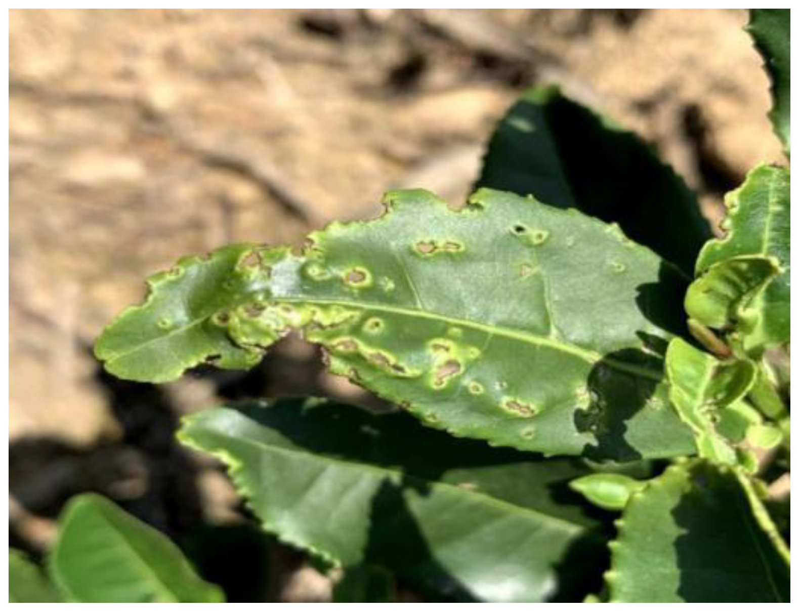
In this study, we first made an on-the-spot investigation in the Maoshan Tea Factory in Jurong, Jiangsu Province, China, and found that in most tea factories in China, the main tea diseases are tea leaf blight (tea tree’s own disease) and Apolygus lucorum (insect pest). This paper selects these two most common tea diseases as the research object. We used a DJI Mavic Air 2 drone (with a 1/2-inch CMOS sensor with 48 MP photos) to shoot over 50 cm of the tea disease area, as well as a handheld iPhone 13 (main camera shooting resolution of 12 MP), and the images obtained were uniformly converted into JPG format. The captured images contained typical features of tea leaf blight (tea tree’s own disease) and Apolygus lucorum (insect pest). The typical characteristics of these tea diseases are shown in Figure 1 and Figure 2.

As shown in Figure 1, this tea disease is caused by Apolygus lucorum, which is a common cell eater. Apolygus lucorum inserts its tentacles into the intercellular space and inside the plant’s cells and then rips the plant cells apart through the tentacles with violent activity. Simultaneously, it secretes saliva outward. The leaves of an infested tea tree will be riddled with numerous holes, cavities, and irregular folds. In extreme cases, the holes become interconnected, and the quality of the tea leaves is severely compromised.

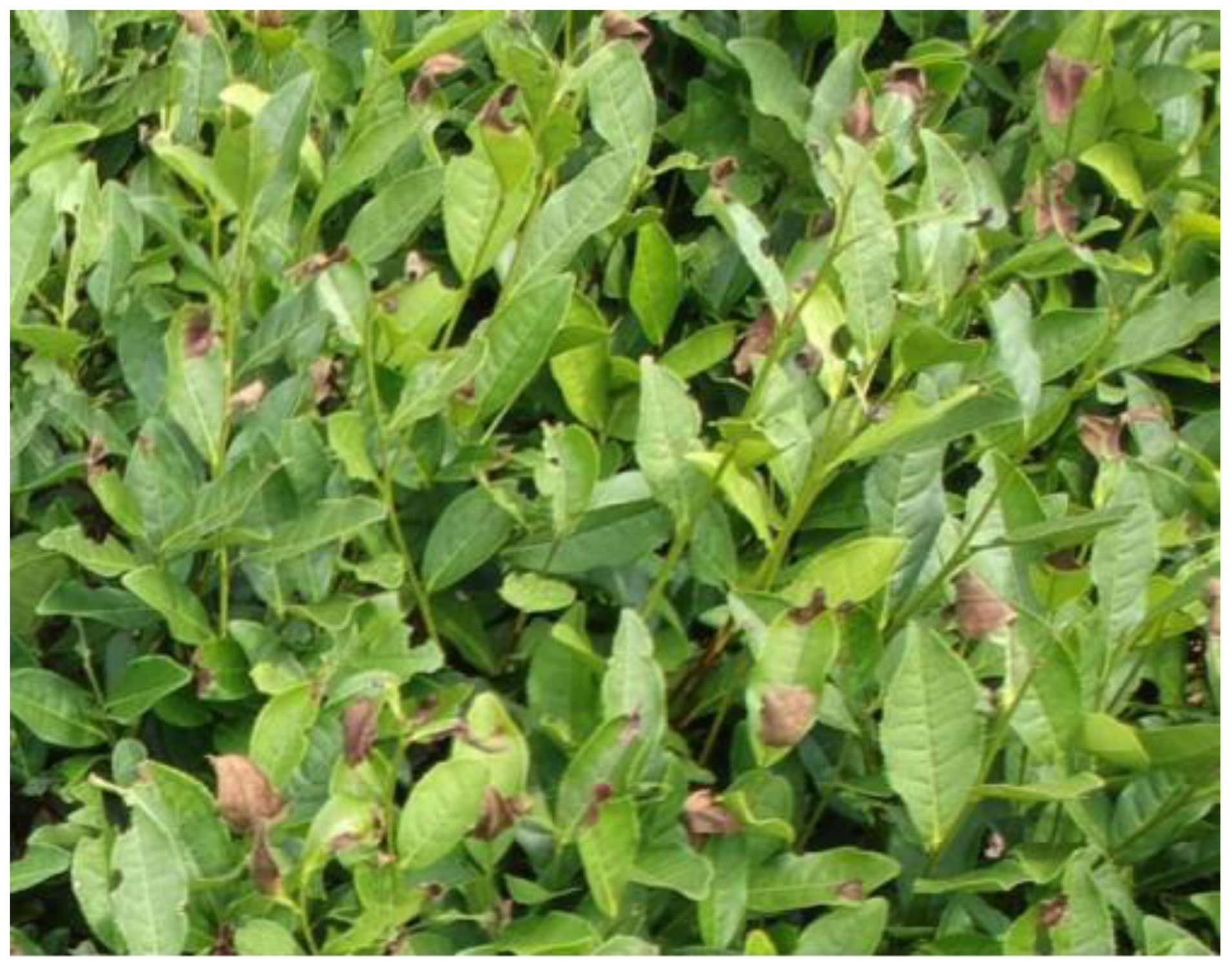
Figure 2 shows the leaf blight of tea. Tea leaf blight mainly damages old leaves and tender leaves. The disease primarily affects the leaf tip or leaf edge, which is semicircular or irregular in shape and predominantly brown in color and causes the tea leaves to senesce prematurely, which has a negative impact on the yield and quality of tea leaves.

The disease areas were manually and accurately labeled. Target detection using deep learning techniques usually divides the dataset into 8:1:1, 7:2:1, or 6:2:2 for training, validation, and testing. However, the dataset in this paper belongs to a small sample dataset, in which the total number of samples is small; in order to make full use of the dataset using enough samples for training to learn the characteristics of a tea disease, we used data augmentation to expand the finished dataset (1000 samples), which was divided into 8:1:1. Since this paper is based on the YOLO framework for model construction, we convert the dataset into the YOLO format.

3. Methods

3.1. Mixed Use Data Enhancement Method

The mixed use of data enhancement methods can not only expand the dataset but also avoids overfitting and improves the robustness of the model, including online and offline enhancement methods.

3.1.1. Offline Data Enhancement

Offline augmentation processes the data prior to model training. It can ensure the consistency of the sample space and avoid the interference of different sample spaces on the detection results. Firstly, the following strategies are used for data enhancement: (1) image rotation: in order to obtain images at different shooting angles, the images were randomly rotated by 90 to 270 degrees; (2) color dithering: in order to obtain images under different light conditions, the chroma, saturation, and contrast of the images were randomly enhanced; (3) sharpen processing: enhances the edge outline of the image to obtain images with different definitions.

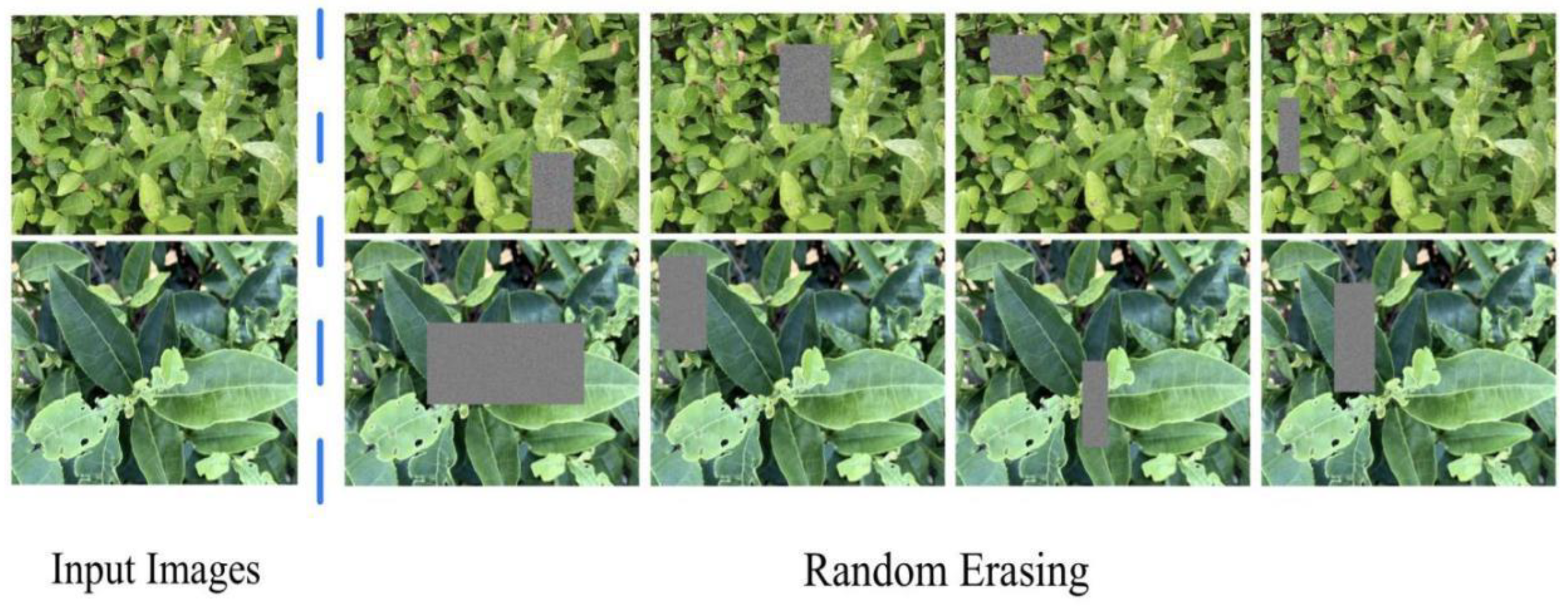
In addition to enhancing the data using image transformations, we also use the random erasing algorithm [29]. A random area in the image is masked so that the model is forced to focus on the pixels outside the masked area. In this way, the training is prevented from falling into a local optimum, and the generalization ability of the model is improved. The effect of random erasing data enhancement is shown in Figure 3.

3.1.2. Online Data Enhancement

The online enhancement method differs from the offline augmentation method in that online augmentation uses data augmentation to transform samples during the training process to ensure the invariance of the number of samples and the diversity of the sample population and improves the robustness of the model by expanding the sample space. Online enhancement strategies include (1) image position transformation: image rotation, translation, and mirror flip; (2) color dithering: image chroma adjustment, image saturation adjustment, and image brightness adjustment.

The number of training samples is the same as the number of images in the training set during online enhancement. In addition to basic image enhancement operations, a mosaic data enhancement approach is used for processing data samples in the training process; namely, multiple pictures are randomly cut and spliced into one picture to be used as a training sample. In the random splicing process, the same picture may have different categories of tea diseases. A richer picture background can bring higher model training efficiency. One example of mosaic data enhancement is shown in Figure 4.

3.2. The Proposed Tea Diseases Detection Model TSBA-YOLO

3.2.1. The Overall Framework of the Proposed TSBA-YOLO

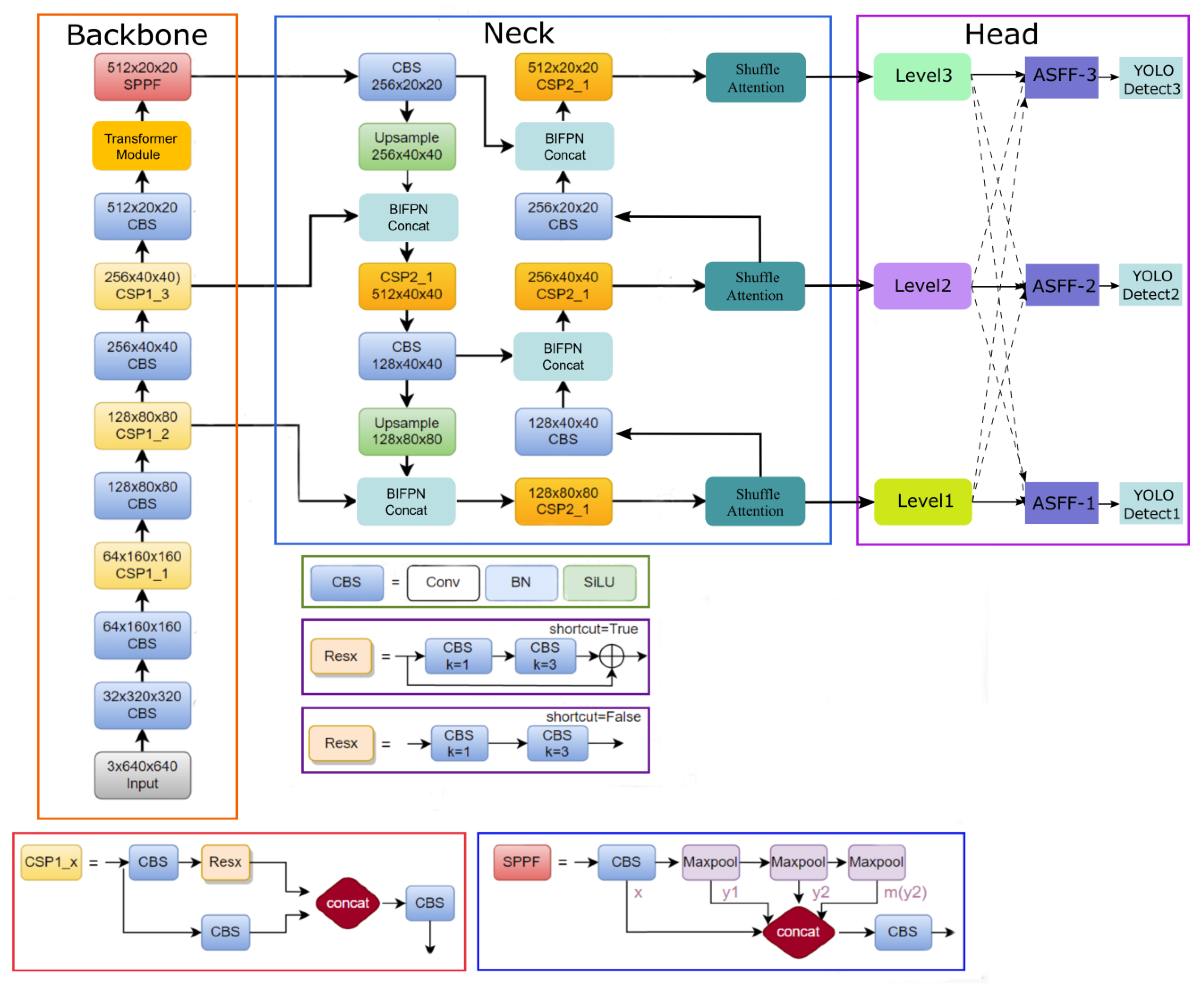
Figure 5 shows the network structure of our improved model: TSBA-YOLO. We have made a series of improvements to the original YOLOv5 algorithm according to the method described above. First, the Transformer module was inserted into the backbone of YOLOv5. The self-attention mechanism of the Transformer is able to enhance the global receptive field of the model, obtain more contextual information, and bring complementary advantages to the original convolution layer, which is more conducive to capturing the global characteristics of tea diseases.

We replace YOLOv5’s feature fusion network PAFPN with BIPFN for more efficient multiscale feature fusion.

The Shuffle Attention (SA) mechanism is integrated into the neck of Yolov5. SA introduces the Channel Shuffle operation while using spatial attention and channel attention simultaneously in blocks. The two types of attention mechanisms are efficiently combined to improve the semantic expression ability of tea disease characteristics. SA can selectively focus on tea disease areas like human vision can, which also improves the detection of small target tea diseases.

Finally, the original detection head of YOLOv5 was replaced with the proposed adaptively spatial feature fusion (ASFF) detection head. The integrated ASFF detection head allows the model to automatically filter useless information to suppress the interference of complex backgrounds on tea disease detection.

Section 3.2.2, Section 3.2.3, Section 3.2.4, Section 3.2.5, Section 3.2.6 of this paper describe each module in detail.

3.2.2. Basic Framework, YOLOv5

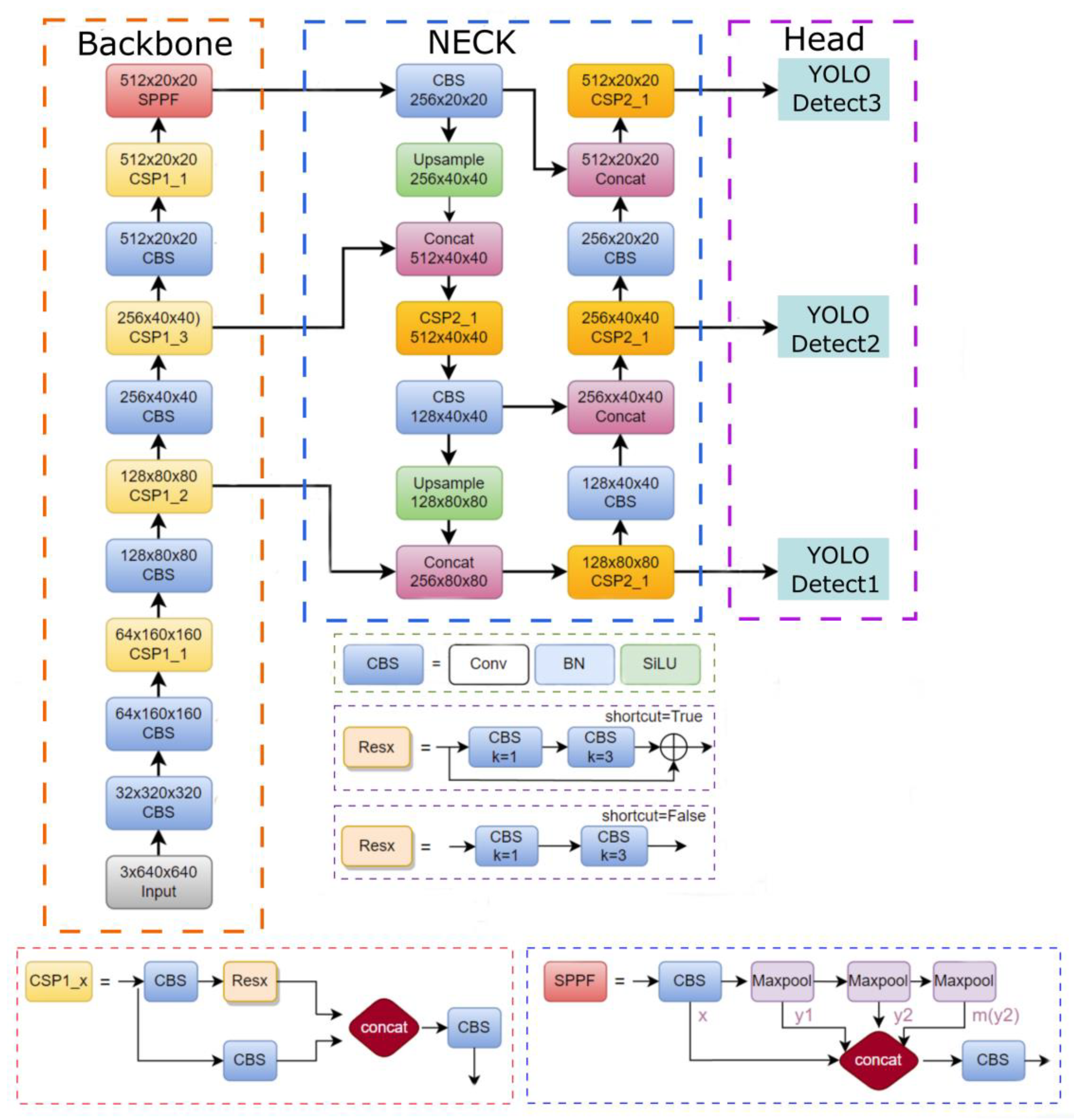
In this paper, YOLOv5 was used as the basic framework for detecting tea diseases, and a series of improvements were made based on it. YOLOv5 is the latest network of the YOLO family, which is a one-stage object detection algorithm. It is mainly composed of a preprocessing module, a feature extraction network, a feature fusion network, and a postprocessing module. The overall structure of YOLOv5 is shown in Figure 6. The SPPF (spatial pyramid pooling fast) module is an improvement on the SPP module [30] in YOLOv4 [31]. In addition to improving the training speed, it can reduce the repeated gradient information and afford better learning abilities. YOLOv5 uses PAFPN [32] as the feature fusion network, i.e., the Concat module in the framework diagram. In the multiscale feature fusion module, three scales of detection layers are set. In addition, the small model weight of YOLOv5 allows for rapid deployment as well as strong advantages in real-time detection on resource-constrained IoT devices. When considering these factors, we chose YOLOv5 as the basic framework for tea disease detection and made a series of innovative improvements to propose the tea disease detection model TSBA-YOLO.

3.2.3. Transformer’s Self-Attention Mechanism

The distribution of various diseases in the image is different: some diseases (such as tea leaf blight) have a small disease area (e.g., on the leaf), and detection relies more on the local information of high-level features. The tea diseases caused by Apolygus lucorum are densely distributed throughout the leaf and need to be inferred from global information. Therefore, global semantic information is very important for the network to improve localization ability. The original backbone of YOLOv5 is mainly based on CNNs. Due to the limitations of convolution operations, CNNs mainly focus on limited perception fields by establishing the relationship between adjacent pixels. There are limitations in capturing long-range interaction information, which lacks long-range semantic relevance, while long-range dependencies are of great importance to networks when focusing on regions of interest and ignoring noise throughout the feature map. In addition, other works have mathematically demonstrated that the effective perception fields of the extracted features are much smaller than the theoretical ones [33], which means that the convolution operation is not realistic in establishing remote dependencies between local image features. In order to overcome the inherent locality of CNNs, some self-attention mechanisms based on locality have been proposed, among which the Transformer is the most outstanding one. In general, Transformer is mainly used for natural language processing and the parallel mining of multiple long-range correlations between temporal information. It has recently been applied in the computer vision domain and achieved impressive results in many visual tasks [34,35,36], such as segmentation [37], tracking [38], image generation [39], enhancement [40], etc. The improvements brought by the visual Transformer networks demonstrate the need for building remote dependencies [41].

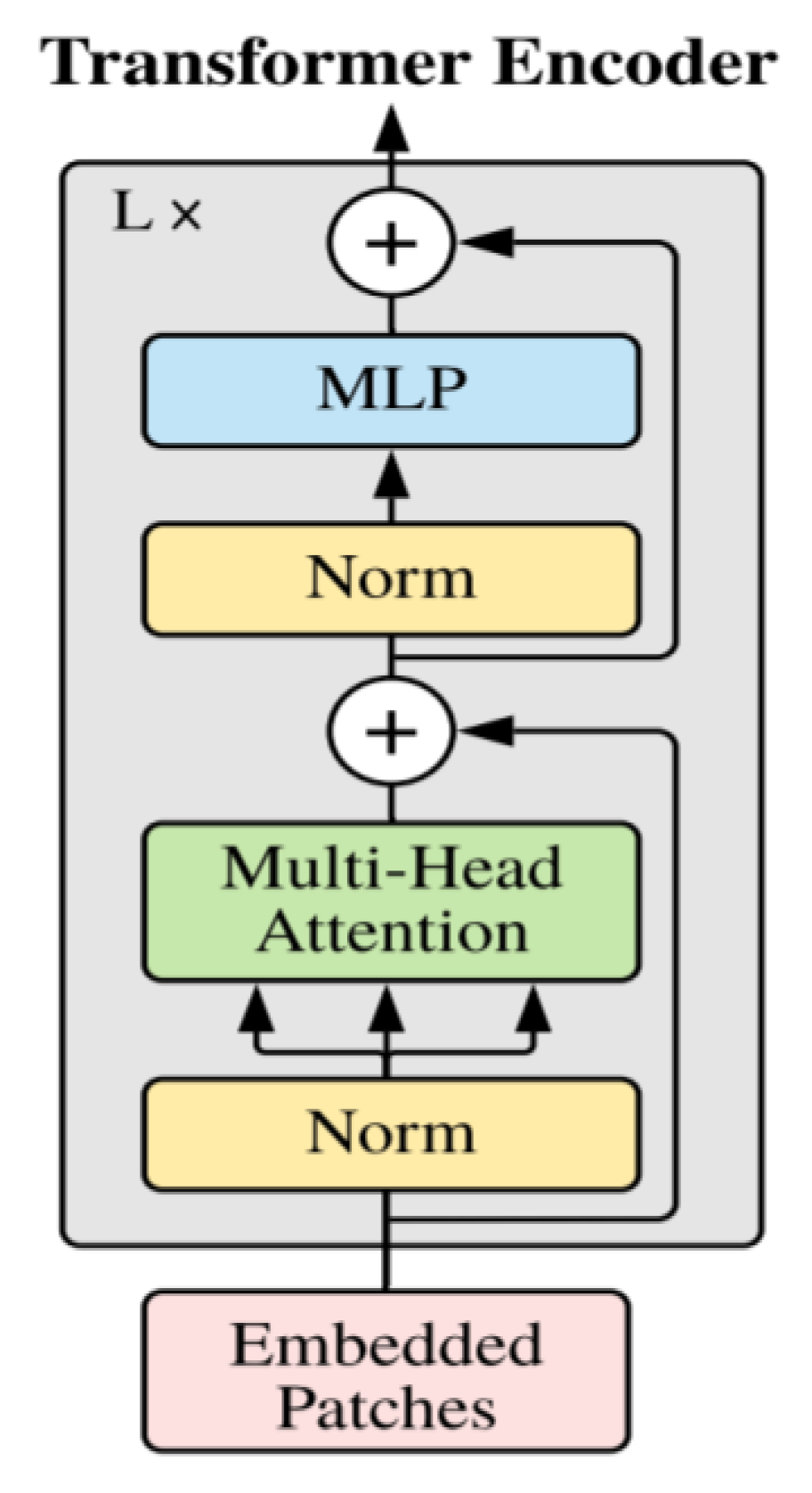
Therefore, in order to make up for the deficiency of the original feature extraction network of YOLOv5, we embed the Transformer encoder with the self-attention mechanism into the CSP module of YOLOv5’s feature extraction network. Transformer’s self-attention mechanism can resolve the problem of long-distance dependence, enhancing the global perception field to capture rich global information and obtain more context information. The structure of the Transformer encoder is shown in Figure 7. The encoder consists of two sublayers. The first sublayer is Multi-Head Attention, which is composed of multiple self-attention modules. The second sublayer is the MLP layer, which is a fully connected layer. Each sublayer uses a residual connection. Adding the normalization layers before and after the two sublayers can make the network converge better and avoid overfitting.

The self-attention mechanism is the core of the Transformer encoder, which can assign different weights according to the importance of particular image regions so that the network can focus on the key information and make the extracted features match the detected targets. In the self-attention mechanism, the embedded patches vector is mapped to three vectors: query ($Q$), key ($K$), and value ($V$) calculated by the dot product $Q$, $K$.The similarity between $K$ and $Q$ is calculated by the dot product. After scaling and softmax normalization to a certain proportion, the similarity value obtained is multiplied by the value vector to obtain the semantic weight. All the semantic weights are weighted and summed to obtain the self-attention feature. Finally, the feature map with abundant information is obtained through MLP processing. The self-attention mechanism is calculated as

$$Z=\mathrm{Attention}\left(Q,K,V\right)=\mathrm{Soft} \max \left(\frac{{QK}^T}{\sqrt{d_k}}\right)V$$

(1)

$Z$ is the self-attention feature; $d_k$ is the scaling factor; $Q$ is the query vector; $K$ is the key vector; $V$ is a value vector.

3.2.4. Multiscale Feature Fusion with BIFPN

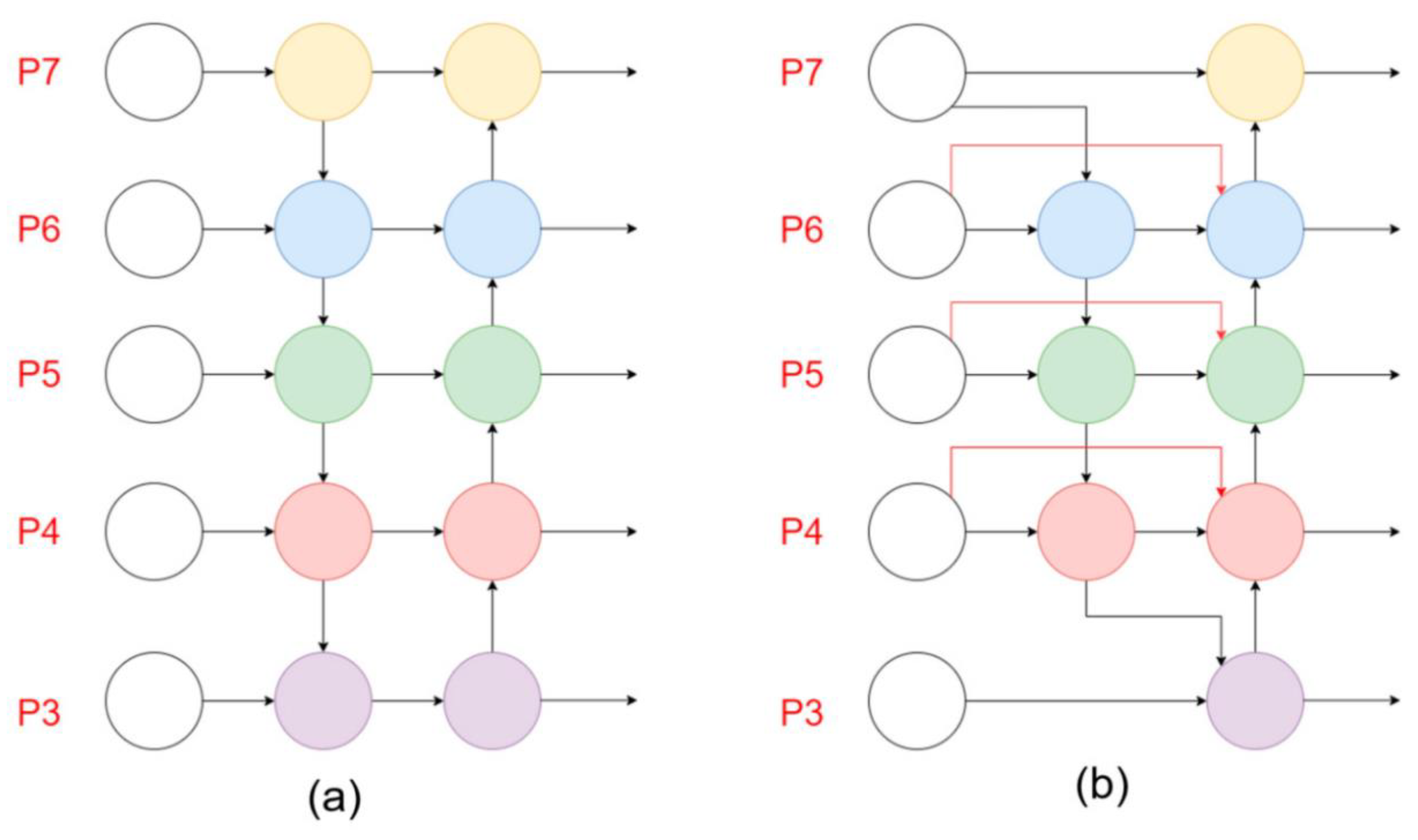
In the collected dataset, there are some differences in shape and size regarding the tea diseases in the same category, which requires feature fusion at different scales. We improved the original multiscale feature fusion network of YOLOv5 by using BiFPN instead of the original PAFPN. BIFPN is a multiscale feature fusion module used in EfficientDet. As shown in Figure 8, BIFPN adds residual connections to the original PAFPN of YOLOV5, with crossconnections to remove the nodes that contribute less to feature fusion in PAFPN, and then adds a jump connection between the input and output nodes at the same scale. Unlike PAFPN, which treats features of different scales equally, BIFPN introduces weights, which can balance the feature information of different scales.

The model (TSBA-YOLO) proposed in this paper follows the idea of BIFPN, which can fuse the multiscale features of tea diseases in an efficient way, enhance the feature representation ability of tea diseases, and reduce the number of parameters of the TSBA-YOLO.

3.2.5. Shuffle Attention Mechanism

We integrated the Shuffle Attention (SA) mechanism module into the original neck of the YOLOv5.SA mechanism, which can selectively focus on the characteristics of tea diseases, which will also improve the detection of small target tea diseases.

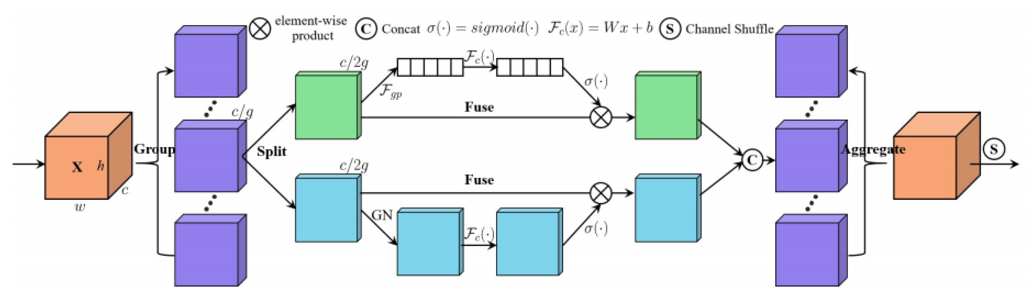
Currently, attention mechanisms can be divided into two categories: channel attention and spatial attention mechanisms. Spatial attention and channel attention capture the dependence relationship between the pixel-level relationship in space and the channels, respectively. Using these two types of attention mechanisms at the same time can achieve better results but at the cost of more computation. The Shuffle Attention (SA) mechanism introduces the Channel Shuffle operation and uses the spatial and channel attention mechanisms simultaneously in blocks so that the two attention mechanisms can be efficiently combined.

Global Average Pooling is used by Shuffle Attention to embed global information to generate the $s\in R^{C/2G\times 1\times 1}$ channel feature, and this can be carried out by passing the spatial direction $H\times W$ through contraction $X_{k_1}$. The calculation formula is as follows:

$$s=F_{gp}(X_{k_1})=\frac{1}{H\times W}{\displaystyle \sum _{i=1}^H{\displaystyle \sum _{j=1}^W{X}_{K_1}(i,j)}}$$

(2)

In addition, SA creates a compact feature through a simple gating mechanism module and sigmoid activation function, providing guidance for adaptive selection and precision. The output of the channel attention is formulated as follows:

$$X_{k_1}^{\prime }=\sigma (F_c(s))\cdot X_{k_1}=\sigma (W_{1}s+b_1)X_{k_1}$$

(3)

In Formula (3), $W_1\in R^{C/2G\times 1\times 1}$ and $b_1\in R^{C/2G\times 1\times 1}$ are for zooming and moving $s$.

Unlike channel attention, spatial attention focuses on “Where”, and complements channel attention. Firstly, group norm (GN) operates on $x_{k_2}$. Then, SA adopts $Fc(·)$ to enhance the representation of $X_{k_2}$. The final output of spatial attention is obtained from the following formula:

$$X_{k_2}^{\prime }=\sigma (W_2\cdot GN(X_{k_2})+b_2)\cdot X_{k_2}$$

(4)

In Formula (4), $W_2\in R^{C/2G\times 1\times 1}$, $b_2\in R^{C/2G\times 1\times 1}$. The Two branches are connected so that the number of channels is the same as the number of channels coming in.

The architecture of SA is shown in Figure 9. The tensor is first divided into G groups, each of which is processed internally using the SA Unit. The internal part of SA is the spatial attention mechanism, as shown in the blue part of Figure 9. The channel attention mechanism used inside SA is shown as the green part of Figure 9. The SA Unit fuses the information within the group via concatenation. Finally, the channel shuffle operation is used to rearrange the groups, and the information flows between the different groups.

We plugged shuffle attention into YOLOv5’s original CNN architecture. Shuffle attention effectively combines the spatial and channel attention mechanisms and can be partitioned and paralleled, which can improve the semantic expression ability of tea disease characteristics. Shuffle attention can help the proposed TSBA-YOLO model extract attention regions and focus on the characteristics of tea diseases.

3.2.6. Adaptively Spatial Feature Fusion Detection Head

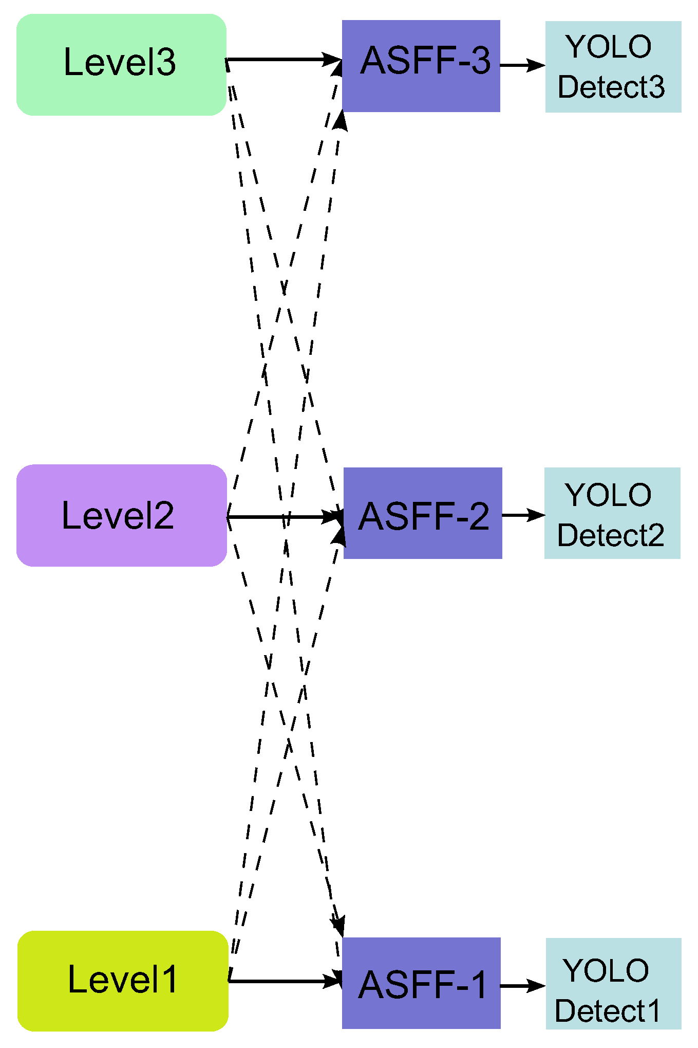
The detection of tea diseases is often disturbed by the complex background of the planting area, and the scale of tea diseases is not fixed, which can make their detection difficult. Therefore, this paper introduces the adaptive spatial feature fusion (ASFF) detection head, which allows the model to automatically filter useless information to suppress the interference of complex backgrounds on tea disease detection and enables the more efficient fusion of disease information at different scales. We replaced the original detection head of YOLOv5 with the ASFF detection head. ASFF will adjust the fusion ratio between different feature layers by adaptive methods and filter spatially conflicting information to suppress the interference of invalid information for detection, thus improving the invariance of the feature ratio, reducing overhead inference and solving the problem of conflicting image spatial information in traditional multiscale feature fusion, effectively improving the multiscale feature fusion of tea disease targets. The structure of ASFF is shown in Figure 10.

Level1, Level2, and Level3 denote the output from the neck in the YOLOv5 network. Taking ASFF-3 as an example, the input of ASFF-3 (after fusion) is the weighted summation of Level1, Level2, and Level3. The result is weight multiplication and addition, as shown in Equation 5:

$$y_{ij}^l={\alpha }_{ij}^l\ast x_{ij}^{1\to l}+{\beta }_{ij}^l\ast x_{ij}^{2\to l}+r_{ij}^l\ast x_{ij}^{3\to l}$$

(5)

In $y_{ij}^l$, the vector (i, j) represents the output feature mapping $y^l$ between the channels, $a_{ij}^l$, ${\beta }_{ij}^l$, $r_{ij}^l$ are the learnable weights representing three different levels up to the l-level feature map; $x_{ij}^{1\to l}$, $x_{ij}^{2\to l}$, $x_{ij}^{3\to l}$ represent the output of a feature map for location. Since the addition method is used, it is necessary to ensure that the number of channels from Level1 to Level3 is consistent with the feature size. The size is adjusted by down-sampling or up-sampling for different levels, and then the Level1, Level2, and Level3 feature maps are subjected to a 1 × 1 convolution to obtain the weight parameter $\alpha$, β, $r$. The weight parameters are then spliced and normalized by the softmax function to map the original input to the range of [0, 1], and the sum is 1. The formula for $a_{ij}^1$ is as follows:

$$a_{ij}^1+{\beta }_{ij}^1+r_{ij}^1=1$$

(6)

$$a_{ij}^1=\frac{e^{{\lambda }_{aij}^1}}{e^{{\lambda }_{aij}^1}+e^{{\lambda }_{\beta ij}^1}+e^{{\lambda }_{\gamma ij}^1}}$$

(7)

3.3. Improved Loss Function

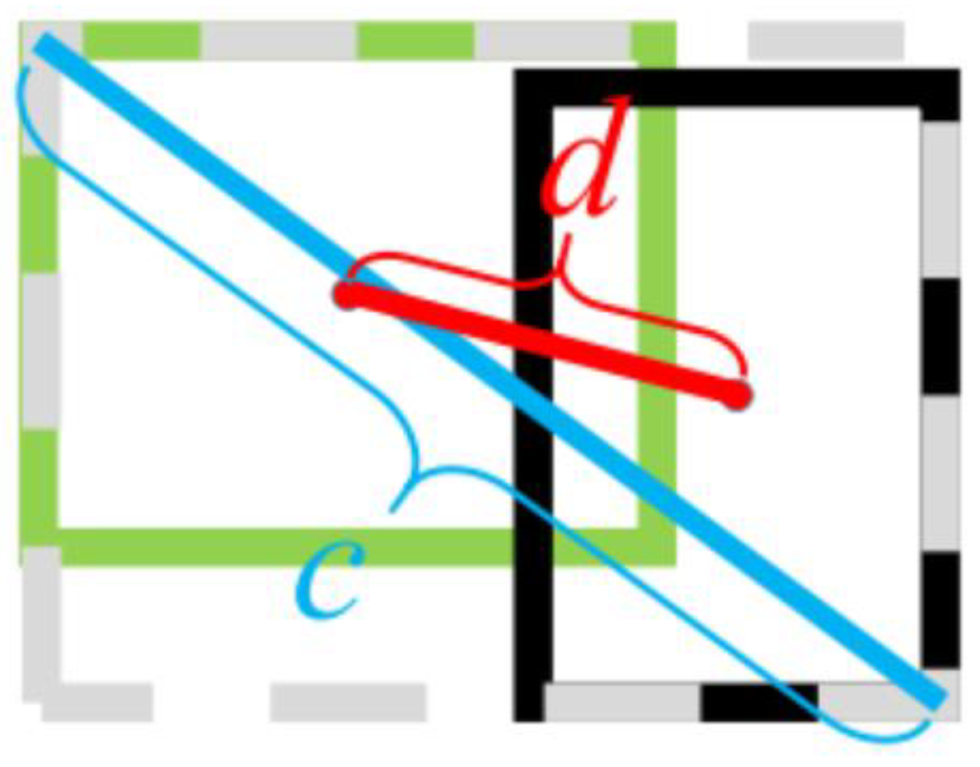
We analyzed the shortcomings of the original loss function of YOLOv5 and adopted an optimized loss function. For the unimproved YOLOv5, CIoU Loss was used as the loss function of the bounding box, and Logits loss function and binary cross entropy were used to calculate the loss of the target score and class probability, respectively. The calculation method of YOLOv5′s CIoU is shown in Formulas (8) and (9):

$$CIoU=IoU-\frac{{\rho }^2(b,b^{gt})}{c^2}-av$$

(8)

$$L_{CIoU}=1-CIoU$$

(9)

$IoU$(intersection over union) represents the intersection ratio of the real bounding box and the bounding box; $c$ represents the shortest diagonal length of the minimum bounding box of the prediction box and the ground truth box, and ${\rho }^2(b,b^{gt})$ represents the Euclidean distance between the center points of the ground truth box and the prediction box. $a$ is a positive balance parameter, $v$ represents the consistency of the aspect ratio of the prediction box and the ground truth box, and the calculation method of $a$ and $v$ is shown in Formulas (10) and (11):

$$v=\frac{4}{{\pi }^2}{(\arctan \frac{w^{gt}}{h^{gt}}-\arctan \frac{w}{h})}^2$$

(10)

$$a=\frac{v}{(1-IoU)+v}$$

(11)

In Equation (10), $h^{gt}$ and $w^{gt}$ represent the height and width of the ground truth box; h and w represent the height and width of the prediction box.

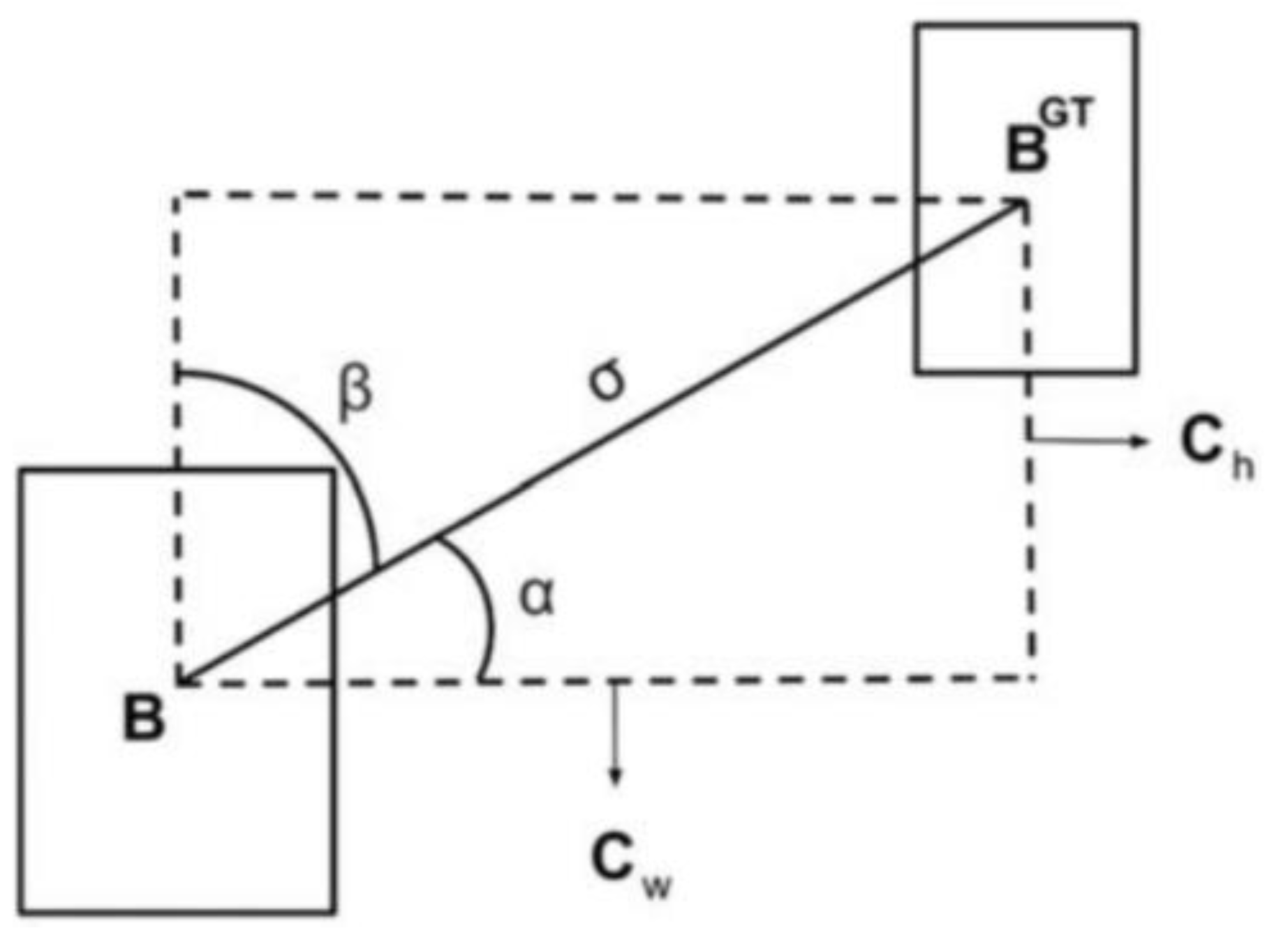
The CIoU scheme is shown in Figure 11. CIoU Loss considers the coverage area, aspect ratio, and center distance, comprehensively, which can measure its relative position well, and solve the problem of optimizing the horizontal and vertical directions of the prediction box, but this method does not consider the direction matching between the target box and the prediction box, which leads to a slow convergence speed. Thus, this paper uses the SIoU loss. As shown in Figure 12, SIoU introduces the vector angle between the target box and the prediction box for optimization.

The calculation method of SIoU is shown in Formulas (12) and (13):

$$SIoU=1-IoU+\frac{\mathsf{\Delta }+\mathsf{\Omega }}{2}$$

(12)

$$IoU=\frac{\left|B\cap B^{GT}\right|}{\left|B\cup B^{GT}\right|}$$

(13)

$B$, $B^{GT}$ represent a prediction box and a ground truth box, $\mathsf{\Omega }$ indicates the shape cost, $\mathsf{\Delta }$ indicates that the angle cost is considered; the distance cost is redefined. The formula of $\mathsf{\Omega }$ and $\mathsf{\Delta }$ is defined as

$$\mathsf{\Omega }={{\displaystyle \sum _{t=w,h}(1-e^{-w_t})}}^{\theta }$$

(14)

$$\mathsf{\Delta }={\displaystyle \sum _{t=x,y}(1-e^{-r{\rho }_t})}$$

(15)

In Formula (14), $w_w=\frac{\left|w-w^{gt}\right|}{\max (w,w^{gt})}$, $w_h=\frac{\left|h-h^{gt}\right|}{\max (h,h^{gt})}$, $\theta$ indicates the degree of concern for $\mathsf{\Omega }$. In Formula (15), ${\rho }_x={(\frac{b_{c_x}^{gt}-b_{c_x}}{c_w})}^2$, ${\rho }_y={(\frac{b_{c_y}^{gt}-b_{c_y}}{c_h})}^2$, of which $\gamma$ is defined as

$$\gamma =1+2{\sin }^2(\arcsin \frac{\max (b_{c_y}^{gt},b_{c_y})-\min (b_{c_y}^{gt},b_{c_y})}{\sqrt{{(b_{c_x}^{gt}-b_{c_x})}^2+{(b_{c_y}^{gt}-b_{c_y})}^2}}-\frac{\pi }{4})$$

(16)

In Formula (16), $b_{c_x}^{gt}$ and $b_{c_y}^{gt}$ are the co-ordinates of the center points of the ground truth box. $b_{c_{\mathrm{x}}}^{}$ and $b_{c_{\mathrm{y}}}^{}$ are the co-ordinates of the center points of prediction box.

By introducing the vector angle between the required regressions, SIoU redefines the distance loss, effectively reducing the degree of freedom of regression, speeding up the convergence of the network, and further improving the accuracy of regression. Therefore, SIoU loss is used as the loss function of bounding box regression in this paper.

3.4. Transfer Learning

The training of DNNs requires a large number of samples to guarantee training performance. Because the number of data samples in this paper is limited, it is difficult to obtain good detection results by training it directly from scratch. Transfer learning is a technique that can apply the acquired knowledge of the known domain to the target domain, which can transfer the trained network model from a large dataset to a new dataset and realize the reuse of the network model parameters and weights on the new dataset.

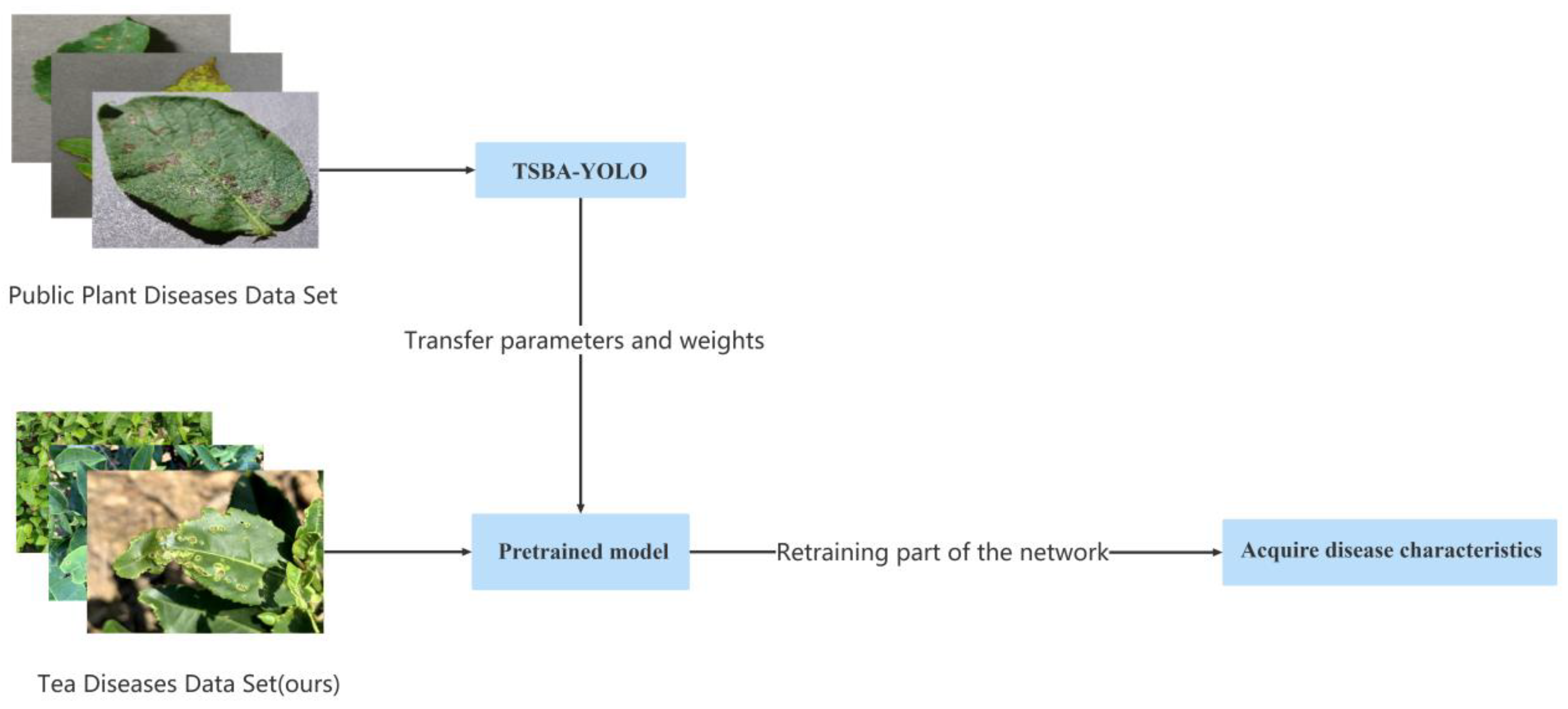
Due to the lack of large-scale image samples of tea diseases and the similarity between the characteristics of tea diseases and other plant diseases, in this paper, a transfer learning method was introduced to improve the performance of the model. Plant Village [42] is a very large dataset of plant leaf diseases, consisting of 54,306 plant leaf images, including 14 species of plants, which are divided into 38 categories according to species and diseases. We used the Plant Village dataset and other plant disease datasets collected from the internet for pretraining. The transfer learning process is shown in Figure 13. First, we used the public dataset to pretrain our improved model, TSBA-YOLO, to get the pre-training weight and then transferred the pretraining weight to our dataset for retraining so as to improve the accuracy and generalization ability of the model.

3.5. Experimental Environment

The training platform used in this paper is a computer equipped with the Windows 10 (64-bit) operating system, an R7 5800H CPU, and an RTX 3060 GPU. Python language was used for programming, and the GPU acceleration framework was CUDA. The training environment and the test environment were the same. Details of the environment used in the experiment are shown in

Table 1. Experimental experiment.

Environment	Details
Operating system	Windows 10 (64-bit)
Programming language	Python (Version 3.8)
CPU	R7 5800H
GPU	RTX 3060
Pytorch version	Pytorch 1.8.2
GPU acceleration framework	CUDA:11.1

.

3.6. Model Evaluation Index

In this paper, precision ($P$) was used to measure the number of correctly predicted samples of tea diseases in the task of detection, ($TP$) accounted for the total number of samples predicted by the model as tea diseases ($TP+FP$), and the formula for $P$ is shown in Formula (17).

$$P=\frac{TP}{TP+FP}$$

(17)

$FP$ indicates the number of samples that are actually free from tea diseases but are misjudged as having tea diseases by the model.

Recall ($R$) represents the number of tea disease samples correctly predicted by the tea disease detection model, ($TP$) accounts for the number of all tea disease samples ($TP+FN$), and the formula is shown in Formula (18).

$$R=\frac{TP}{TP+FN}$$

(18)

$FN$ indicates the number of samples that actually have tea diseases but are misjudged by the model as having no tea diseases.

Average Precision ($AP$) was used to represent the identification accuracy of each tea disease, and the calculation formula of $AP$ is as shown in Formula (19).

$$AP={\displaystyle {\int }_0^{1}P(R)}dR$$

(19)

Mean Average Precision ($mAP$) was used to represent the average identification accuracy of all categories of tea diseases, and the calculation formula is shown in Formula (20).

$$mAP=\frac{1}{c}\times {\displaystyle {\sum }_{k=1}^c{(AP)}_k}$$

(20)

$k$ is the total number of categories of tea diseases, and $c$ is the serial number of each category.

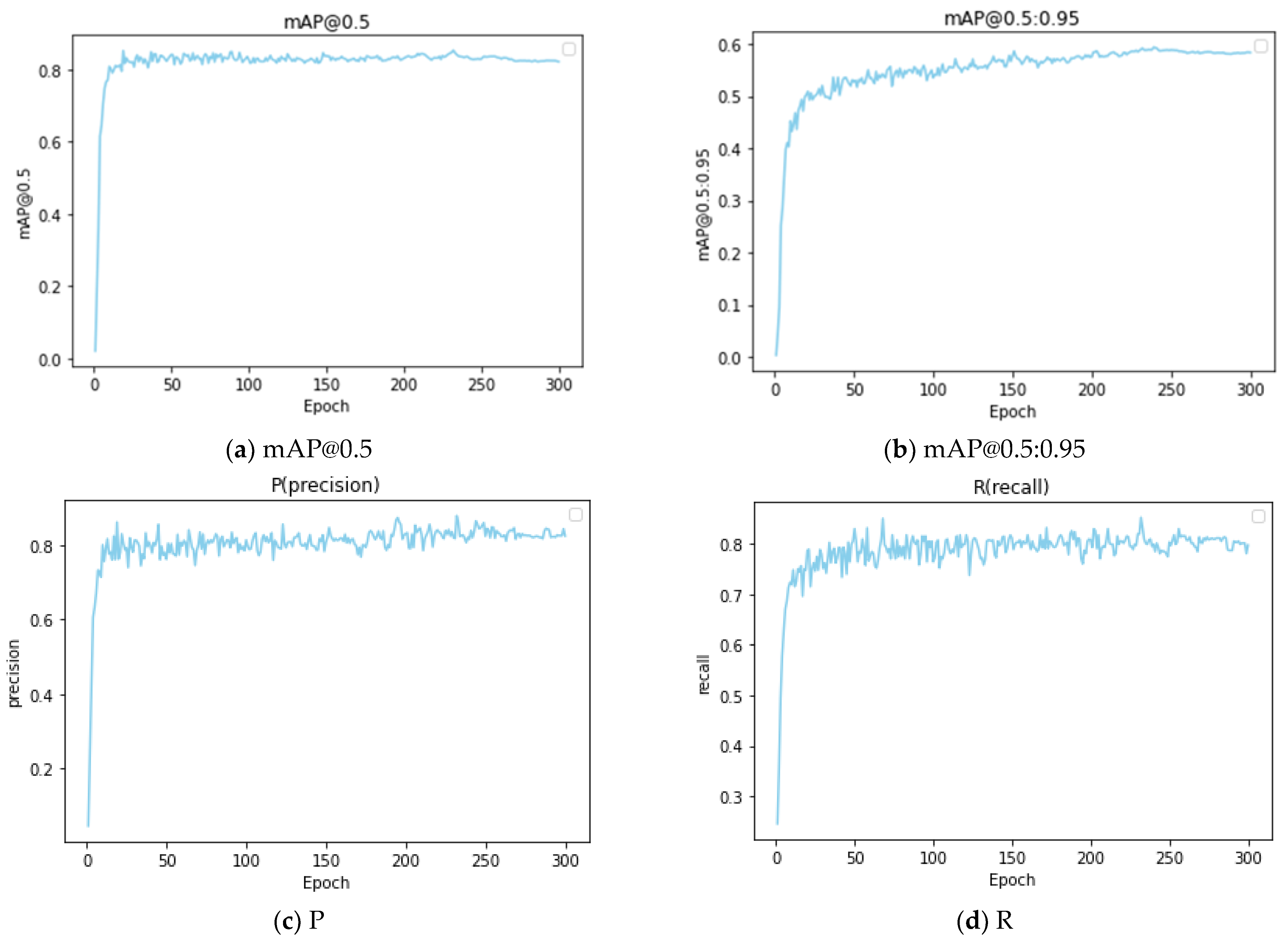
In object detection, it is generally considered that the intersection ratio between the actual bounding box and the predicted bounding box is ≥0.5, so we choose mAP under the condition of IoU = 0.5:mAP@0.5, and the average mAP: mAP@0.5:0.95 over different IoU thresholds (from 0.5 to 0.95) to evaluate our tea disease detection model, which is more demanding on accuracy.

FPS (frames per second) was used to evaluate the speed of detecting the tea diseases, that is, the number of pictures that can be processed per second.

4. Results and Discussion

4.1. Training

In the process of training TSBA-YOLO, the stochastic gradient descent method (SGD) was used; the learning rate was adjusted according to the linear scaling principle, the initial learning rate(lr) = 0.001, and the pretraining weights obtained from transfer learning were trained for 300 rounds (Epoch).

Figure 14 shows the convergence process of each evaluation index in the training process of the tea disease detection model TSBA-YOLO. It can be seen that the convergence speed of TSBA-YOLO is relatively fast, and it converges to a relatively ideal effect by the 15th Epoch. The mAP@0.5 of the 232nd Epoch reached the best value of 85.35, after which the accuracy did not improve. Therefore, we selected the weight obtained from the 232nd Epoch training as our optimal weight, which had the highest accuracy.

We evaluated the optimal weight of the model, drew the PR curve, and calculated the AUC-PR according to the evaluation results. The PR curve is shown in Figure 15. The value of AUC-PR is 0.8535.

4.2. Ablation Experiment

In this paper, ablation experiments were carried out to prove the effectiveness of each module, and the evaluation indicators mentioned above were used to evaluate the improvement effect of the improved model, as compared with the mainstream target detection model. The results are shown in

Table 2. Ablation experiment results.

Model	mAP@0.5 (%)	mAP@0.5:0.95 (%)	$\mathit{P}$ (%)	$\mathit{R}$ (%)	FPS
SSD	76.21	52.02	75.01	76.34	45
Fast R-CNN	78.01	55.01	77.68	77.01	19
EfficentDet	78.99	53.98	77.98	76.79	36
Yolov5	79.32	54.34	79.01	79.03	55
Yolov5 + Transformer	81.56	56.00	82.01	81.99	53
Yolov5 + Transformer + BIFPN	82.32	56.01	84.11	83.01	54
Yolov5 + Transformer + BIFPN + SA	84.01	57.38	85.81	83.03	52
Yolov5 + Transformer + BIFPN + SA + ASFF	85.26	58.99	87.25	85.01	51
Yolov5 + Transformer + BIFPN + SA + ASFF + SIoU(TSBA-YOLO, ours)	85.35	59.17	87.83	85.27	51

.

Through the ablation experiments, we found that TSBA-YOLO, which integrates the Transformer self-attention module, the BIFPN feature fusion network, and the Shuffle Attention module, by using the adaptive spatial feature fusion detect head, improved the accuracy of tea disease detection. Each of the modules used for the improvements increased the detection accuracy. The integrated Transformer module first improved the average accuracy (mAP@0.5) by 2.24, and the integrated BIFPN accuracy improved it by 0.76 on top of that. Thereafter, the integrated SA and ASFF modules improved the accuracy to 84.01 and 85.26. Using the improved loss function SIoU training also slightly improved the accuracy. The final average accuracy of TSBA-YOLO (mAP@0.5) reached 85.35, which is 6.03 higher than that of YOLOv5.mAP@0.5:0.95; P and R were both higher than the native YOLOv5. All metrics were higher than the mainstream target detection models.

In terms of real-time detection, the detection speed of TSBA-YOLO is almost the same as that of the original YOLOv5. The improved TSBA-YOLO inherits the advantages of YOLOv5 in terms of detection speed, which is due to the fact that the module integrated and introduced in this paper is lightweight and does not need to consume too many computing resources, and the FPS reaches 51, that is, it can process 51 frames per second, which meets the needs of real-time detection and is much higher than other mainstream target detection models.

4.3. Detection Performance and Comparative Analysis

By comparing the detection results, we found that the recognition performance of the improved TSBA-YOLO model is much better than that of the original YOLOv5. Especially, the ability of noncomplex background interference and global feature extraction improved a lot, and the number of undetected diseases was also smaller. The effectiveness of each module we designed was further verified by comparing the test results, and some of the test results are shown below.

As shown in Figure 16a–e, with the complex background interference from the tea planting area, YOLOv5 mistakenly regards the dead leaves on the ground as tea disease (tea leaf blight), while TSBA-YOLO can resist the interference of a complex background and successfully detects the small target leaf blight with insufficient appearances in the upper right corner. For the same disease site, the confidence level of TSBA-YOLO is also higher than that of YOLOv5. SSD fails to detect all tea disease targets. Fast R-CNN and EfficentDet are both disturbed by dead leaves.

As shown in Figure 17a–e, in the same image, there are many tea disease (Apolygus lucorum) targets, and some tea disease targets have insufficient appearances. YOLOv5 detected three fewer targets than TSBA-YOLO and had false detection. TSBA-YOLO can detect small tea disease targets with insufficient appearances. SSD, Fast R-CNN, and EfficentDet all missed some tea disease targets.

Similarly, as shown in Figure 18a–e, in the detection of tea leaf blight (most are small targets), YOLOv5 also has more missed detections than our tea disease detection model TSBA-YOLO. SSD, Fast R-CNN, and EfficentDet all failed to detect some small targets.

Because the tea disease Apolygus lucorum densely appears on a single tea leaf and usually occupies the whole leaf, it is necessary to infer this from global information. Figure 19a shows the detection result of YOLOv5. YOLOv5 has two misjudgments because the local characteristics of the two tea leaves are similar to those of Apolygus lucorum. As shown in Figure 19b, TSBA-YOLO has no misjudgment, and the confidence level of detection reaches 0.91, which is 9.6% higher than that of YOLOv5. This is due to the integration of the Transformer module providing TSBA-YOLO with strong global modeling capabilities and self-attention mechanism. As shown in Figure 19c–e, SSD fails to detect the tea disease target, and Fast R-CNN and EfficentDet both made false detections.

5. Conclusions

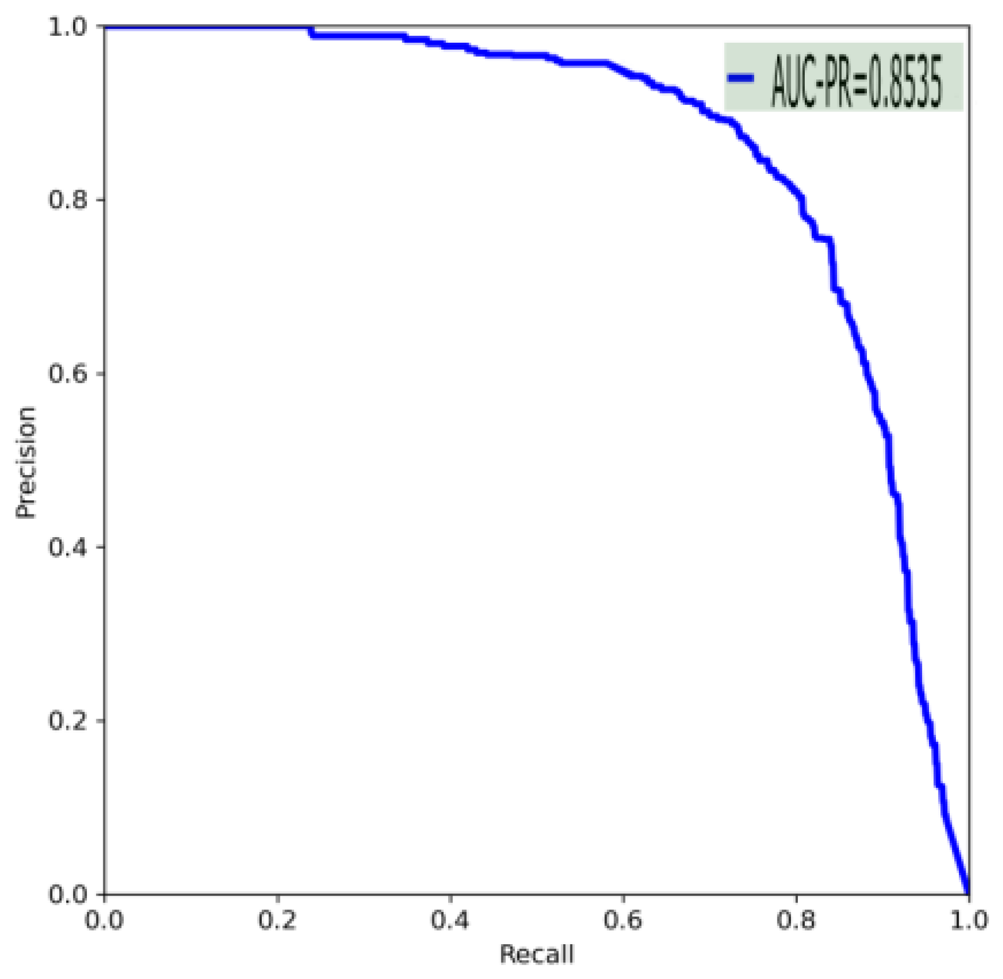
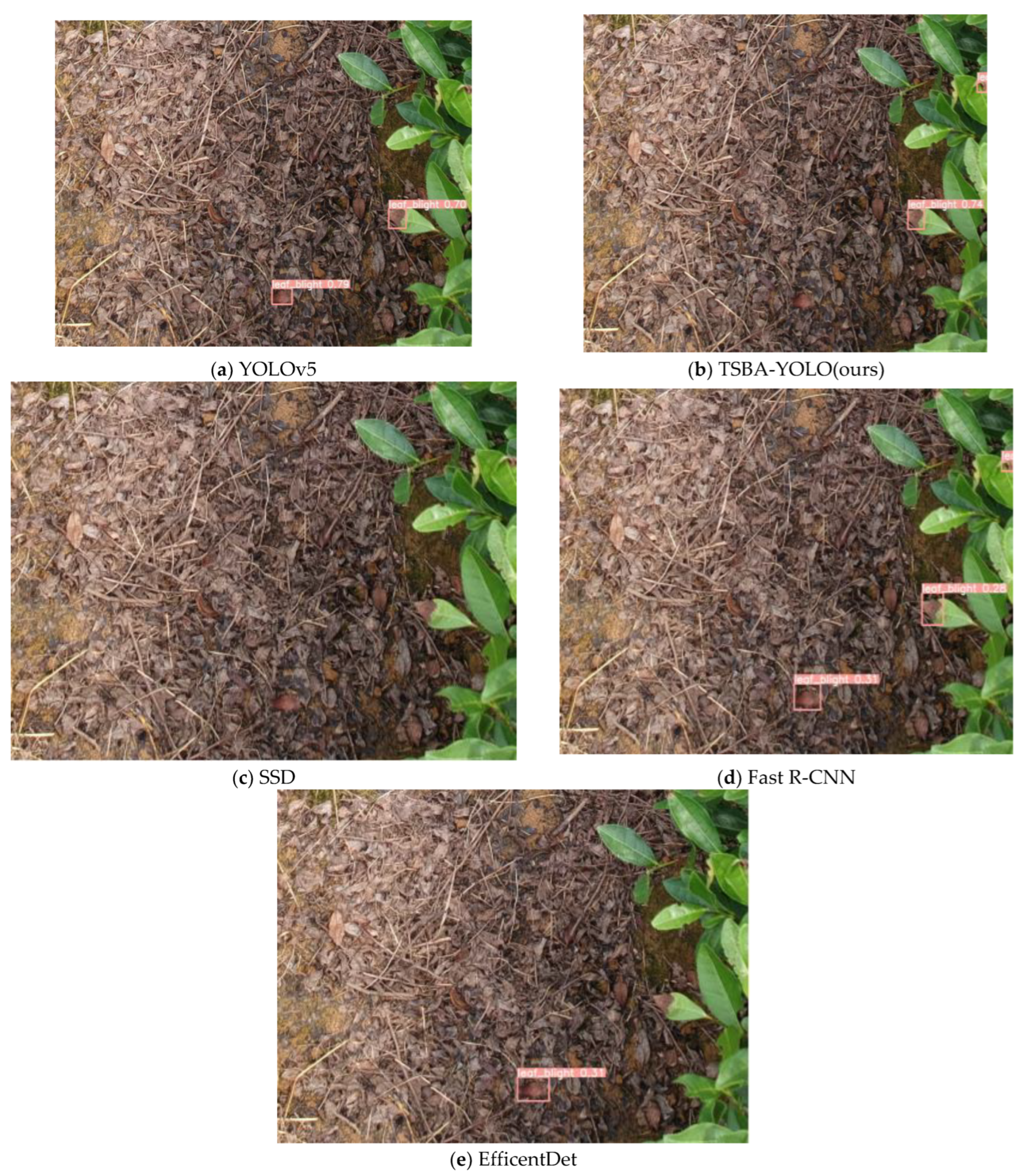
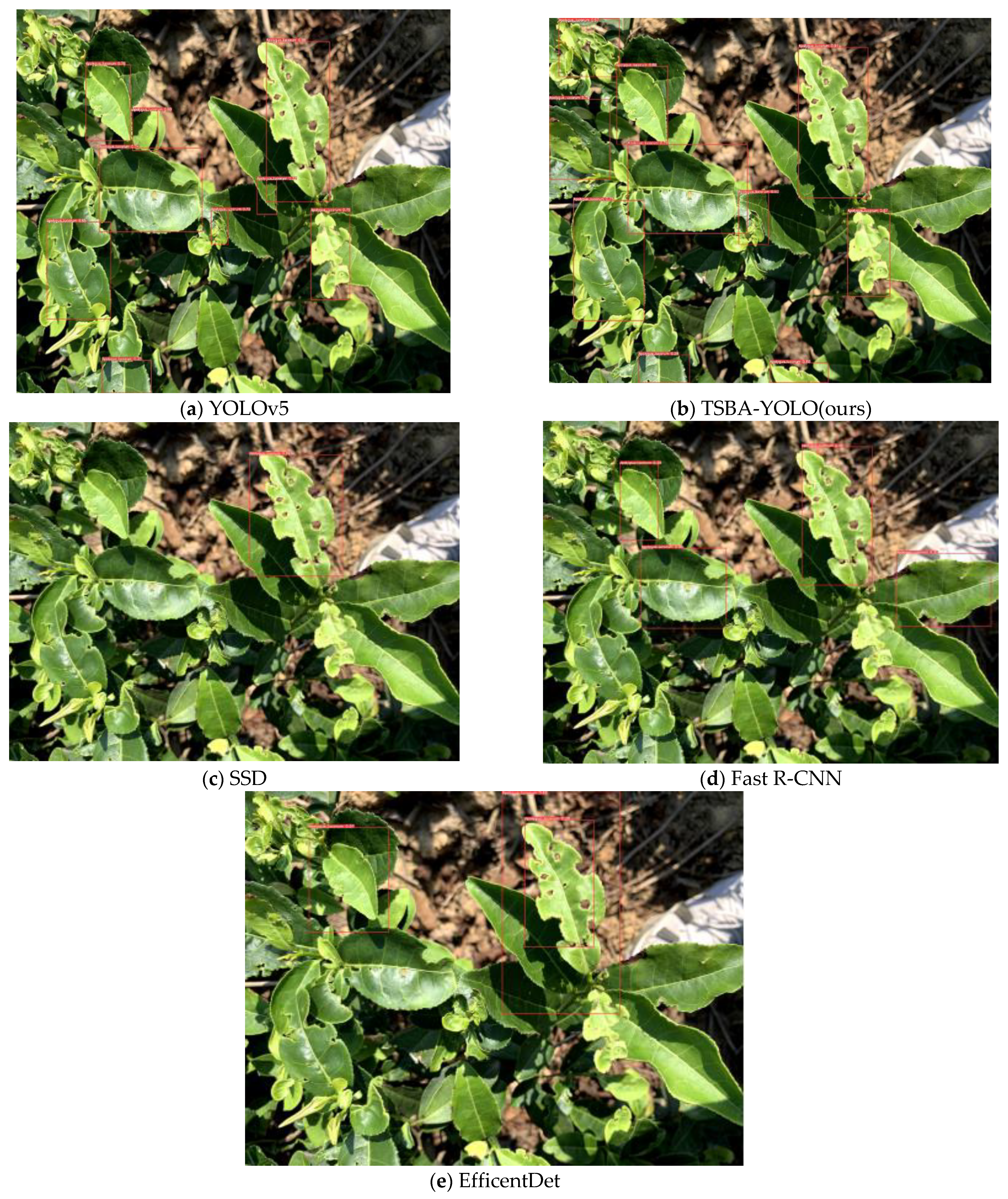
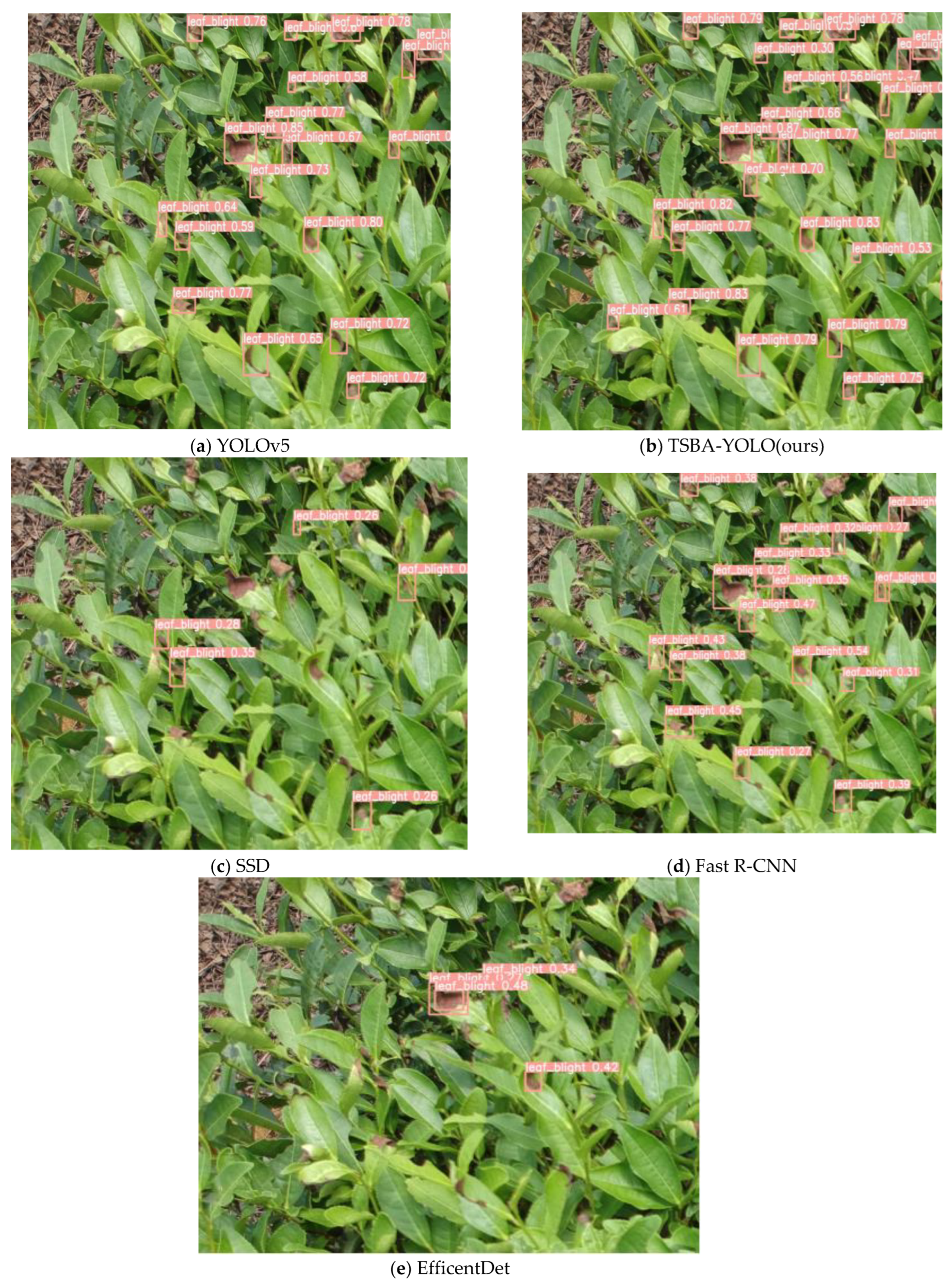
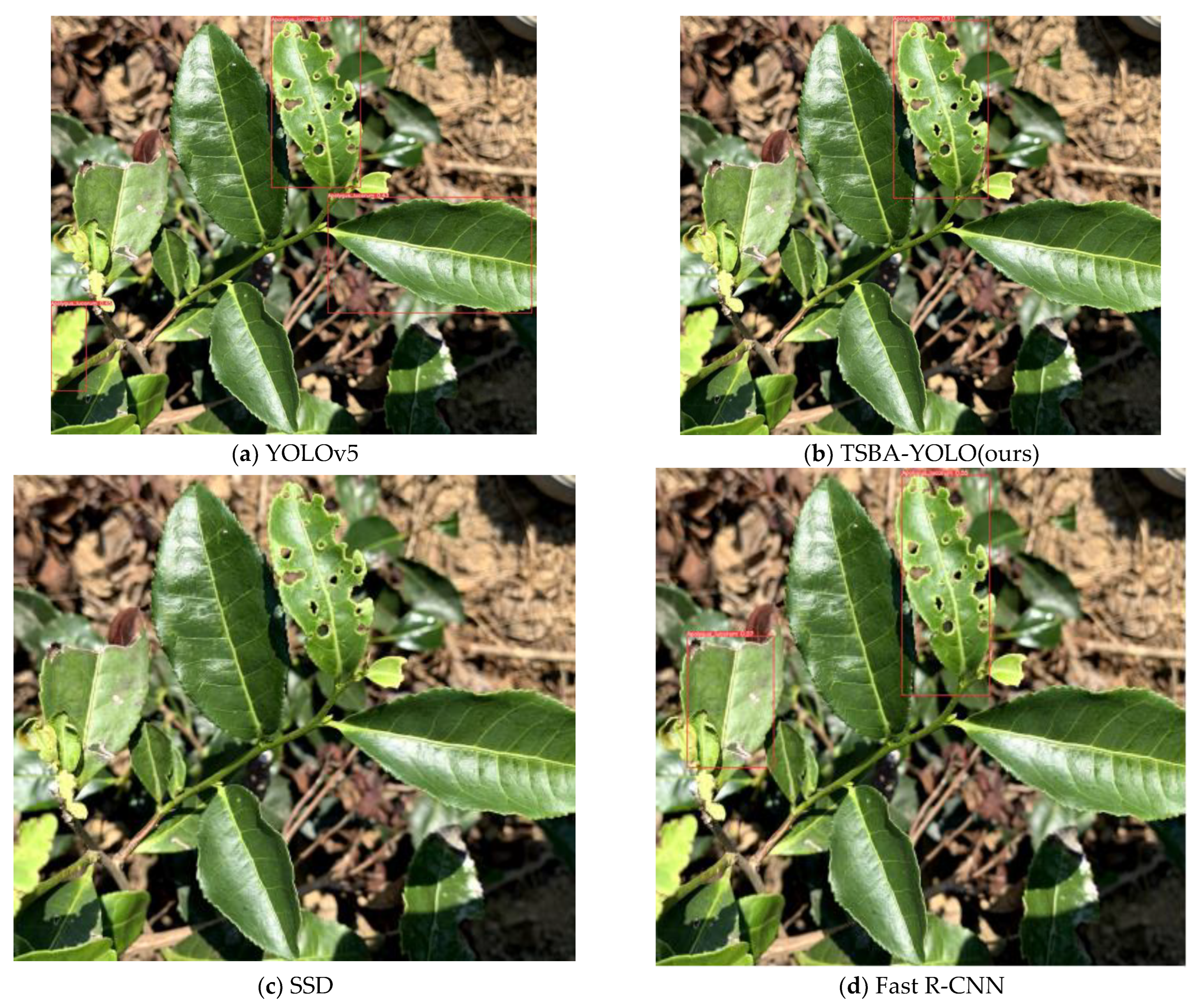
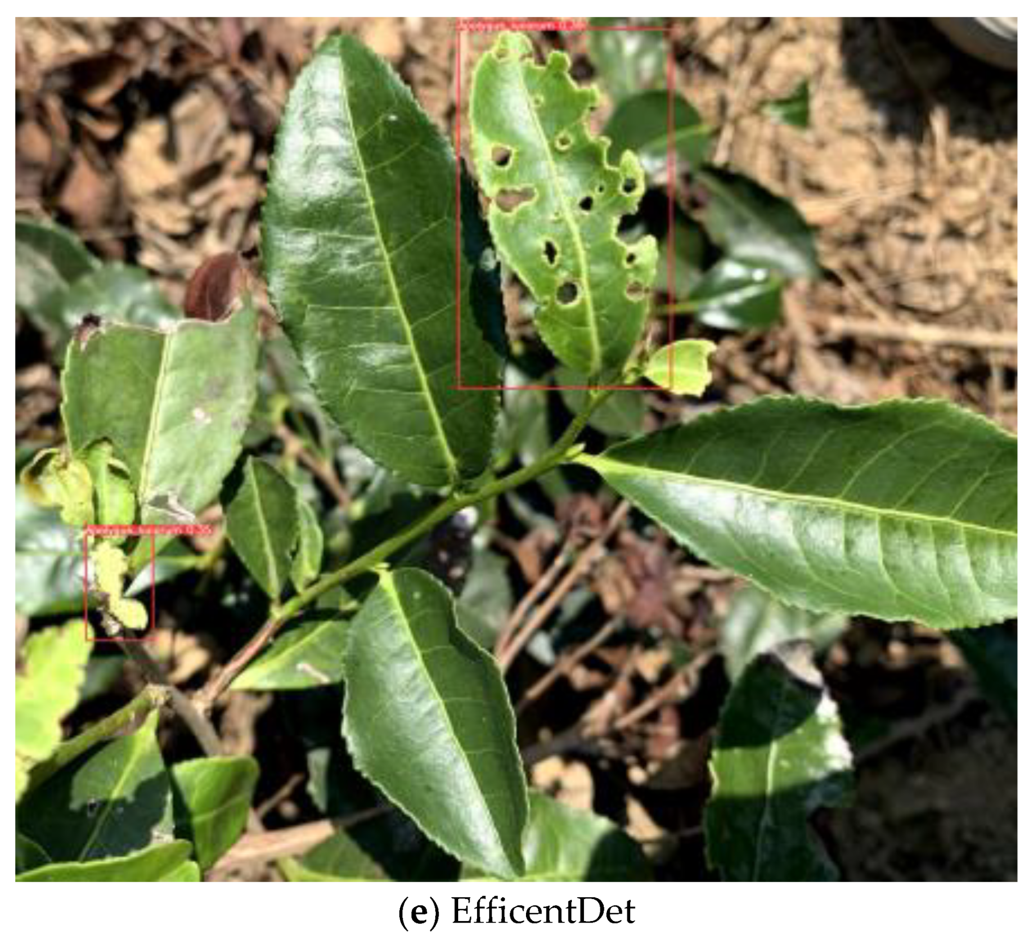
The shape and scale of tea diseases are variable; tea disease targets are usually small, and the process of their intelligent detection is easily disturbed by the complex background of the growing area. In addition, some tea diseases are concentrated in the entire area of the leaves, needing to be inferred from global information. Common generic target detection models can hardly solve these problems. In this paper, a real-time detection model of tea diseases, TSBA-YOLO, was designed based on the common tea diseases of tea plant leaf blight and Apolygus lucorum. Firstly, aiming at the problem of insufficient tea disease datasets, data enhancement methods were used to expand the samples. The random erasing algorithm was used to cover part of the information of the image randomly, forcing the tea disease model to learn the features outside the region for recognition, which can effectively avoid the model falling into a local optimum and improve the generalization ability of the model. The self-attention mechanism of Transformer and convolution layer were introduced into the feature extraction network to form complementary advantages, which enhanced the global perception field of the model so that more contextual information could be obtained. The PAFPN of the YOLOv5 detection framework was changed to a BiFPN structure, thus enabling the effective fusion of multiscale targets. Secondly, we integrated the Shuffle Attention (SA) mechanism to efficiently improve the semantic expression ability of tea disease characteristics. Therefore, TSBA-YOLO can focus more on the field of tea disease and will also focus more on small-target tea diseases. The integrated adaptively spatial feature fusion (ASFF) detection head could further improve multi-cale feature fusion and automatically filter useless information to suppress the interference of complex backgrounds from tea disease detection. The original loss function was optimized using SIoU. SIoU introduces a vector angle between the required regressions, redefines the distance loss, effectively reduces the degree of freedom of the regression, speeds up the convergence of the network, and further improves regression accuracy. Finally, the proposed transfer learning strategy was used to train the model, which further accelerates the convergence speed of the model and improves the accuracy and robustness of tea disease detection in a small sample case. The average accuracy (mAP@0.5) of TSBA-YOLO improved to 85.35, which is much higher than that of the unimproved YOLOv5 and other mainstream object detection models. Through ablation experiments, the effectiveness of each module of TSBA-YOLO was verified, and the accuracy was improved. The detection speed of TSBA-YOLO reached 51FPS, which meets the needs of real-time detection. By comparing the detection results, it was found that the ability of TSBA-YOLO to resist complex background interference and the ability to extract global features is much better than that of YOLOv5, and the number of undetected pests and diseases is lower.

TSBA-YOLO can be deployed at the edge of UAVs and video surveillance equipment to detect tea diseases in real-time and can also be deployed in the servers. It can replace the traditional manual inspection of large areas in tea factories and detect tea diseases in a timely manner so as to spray pesticides to minimize economic losses. TSBA-YOLO can also migrate to other plant disease detection. In the future, we will use the method of model integration to further improve the accuracy of tea disease detection by using multiple models to jointly infer a tea disease area and fuse the detection results, which will further solve the problem of missed detection and false detection.