Effect of Land Use and Land Cover Change on Plant Diversity in the Ghodaghodi Lake Complex, Nepal

Abstract

The Ghodaghodi Lake Complex is a Ramsar site, Nepal’s first bird sanctuary, and has significant ecological and economic values. The lake complex is in the western part of the lowland of the Terai region. Numerous studies indicate a relation between the normalized difference vegetation index (NDVI), land use, and land cover with plant diversity. However, the association between terrestrial plant diversity and NDVI in the Ghodaghodi Lake Complex is unknown but has important implications due to potential land use changes. We aimed to understand the relationship between plant diversity and NDVI in the Ghodaghodi Lake Complex. We performed a vegetation survey using a simple random sampling methodology. Shannon–Wiener’s diversity index (H’) was calculated from the field data, and Landsat images were used to compare land use and land cover changes and calculate NDVI values for 2000 and 2022. The image classification shows that forest cover in April and December 2000 was 71.1% and 58.5%, respectively, and was the dominant land cover in the study area. In contrast, agriculture occupied 18.8% and 27.3% in April and December 2000, respectively, and was the primary land use. Forests covered the most land in April (64.8%) and December (65.3%) of 2022. Likewise, agriculture was a widespread land use. We found a significant correlation (r = 0.80, p < 0.05) between the NDVI and plant species diversity, as the NDVI explained 65% of plant species diversity. There was a decrease in forest cover from 2000 to 2022. The strong correlation between the NDVI and vegetation species diversity shows that the NDVI can be a substitute for plant diversity. Our findings show that increased NDVI corresponds to increased plant species diversity and that the lake complex had more plant diversity in 2022 than in 2000, despite a decrease in forested lands.

1. Introduction

Land use and cover are often used interchangeably, but their meanings differ [1]. Land use refers to human activities of how it is worked upon and managed, such as residential, industrial zones, or agriculture. In contrast, land cover is a physical characteristic of Earth’s surface, such as forests, agriculture, wetlands, or lakes, solely created by human activities [2]. Land use and land cover change (LULCC) analyses focus on how the land has been used, what types of changes are predicted in the future, and the various driving forces and processes behind these changes [3]. The main driver of LULCC is anthropogenic activities, such as socio-economic activities. Due to rapid human settlement, the land use/cover effect has become an emerging issue worldwide. LULCC responds to social and ecological processes in the landscape.

Vegetation species diversity measures the health of plant communities and ecosystems and influences other biotic communities [4,5,6,7,8] and ecological processes [9,10,11,12,13]. Anthropogenic activities and land use affect plant diversity [14,15]. Therefore, LULCC is essential in assessing plant diversity. Land use and land cover are correlated; thus, a change in one factor affects the other [2]. LULCC impacts biodiversity, water and radiation budgets, trace gas emissions, and other climatic processes [16]. LULCC affects the local, regional, and global climate.

Vegetation species diversity and spectral information from the image are essential in assessing biodiversity. The biodiversity assessment is based on the spectral resolution of the data [17]. Landsat, the remote sensing system, analyzes spectral information collected from visible, near-infrared, and the middle region related to plant properties [18]. Near-infrared and red bands are used for estimating tree diversity [19,20,21]. Plant diversity and normalized difference vegetation index (NDVI) are also strongly correlated in the savannah biomes [22]. NDVI is sensitive to critical environmental factors, such as rainfall, that affect biodiversity [23]. The NDVI analyzes energy in an ecosystem as primary productivity that defines spectral patterns in plant diversity [20,24]. NDVI measures the energy entering the ecosystem through primary productivity [25]. Because of this relationship between primary productivity and NDVI, the NDVI predicts a change in species richness [19]. Gould [19] studied that this change in the NDVI corresponds with a change in species richness in the arctic landscape of Canada. A positive correlation between the NDVI and vegetation species diversity was presented by Gould [19] and Levin et al. [25]. However, a study in Argentina indicated a poor relationship between the NDVI and secondary productivity [26].

Historical spatial attribute data allow for assessing changes in plant species diversity over time [27]. Walter [28] presented a positive correlation between plant species richness and NDVI in California, USA. Zhang et al. found that the NDVI and net primary productivity (NPP) are correlated. Because of this relationship between the NDVI and NPP and NPP and species richness, researchers showed a connection between the NDVI and species richness [29]. Wang et al. [30] studied a positive correlation between the NDVI and plant diversity in grasslands. Similar results were found by Madonsela et al. [22] in savannahs, Pouteau et al. [31] in rainforests, and Levin et al. [25] in mountainous regions. NDVI explained up to 87% variation in species diversity for a particular vegetation type, landscape, or region [32]. The normalized difference vegetation index (NDVI) ranges from −1 to 1. The negative value represents the surface covered with clouds and water, the positive value is vegetation, and zero shows bare land [33]. An area rich in vegetation reflects a higher NDVI, while the negative value of NDVI represents no vegetation [34]. The NDVI is less sensitive to soil differences, so it is less sensitive to solar elevation. Still, it is susceptible to green vegetation [35].

Due to plant diversity’s role in promoting the biodiversity of other taxa and the ecosystem services they provide [4,6,7,11,13], we thought it prudent to study plant diversity in the Ghodaghodi Lake Complex due to potential perturbations on site. The study’s general objective is to show the effect of LULCC on plant diversity in the Ghodaghodi Lake Complex, Nepal. The study’s goals are to (1) assess the LULCC, (2) show the relation between the NDVI and vegetation species diversity, and (3) assess the terrestrial plant biodiversity in the Ghodaghodi Lake Complex. We assume that there is a linear relationship between the NDVI and plant diversity.

2. Materials and Methods

2.1. Study Area

The Ghodaghodi Lake Complex (GLC) lies in the Kailali district of the Sudur Pashchim Province of Nepal (Figure 1). It is in the southwestern part of Terai, having spatial extents between latitude 28°41′17″ N and longitude 80°56′47″ E, and the elevation is 205 m (about 672.57 ft). The wetlands cover approximately 2500 ha [36]. The Ramsar site comprises 14 large and small lakes and ponds separated by a hillock [37]. On the lower slope of Siwalik, the lake complex is surrounded by tropical deciduous forests [38]. Ghodaghodi (138 ha), Nakharodi (70 ha), and Baishawa (10 ha) are the major lakes of the complex [37]. The GLC is a Ramsar site, a key biodiversity area, and Nepal’s first bird sanctuary. It supports a significant population of fishing cats (Prionailurus viverrinus) (vulnerable), mugger crocodiles (Crocodylus palustris) (vulnerable), a national biodiversity indicator species, Cotton Pygmy Goose (least concern), 319 birds, and 29 fish species [39]. The Basanta forest corridor enables wildlife movement from Siwalik to the Western Terai Complex: Bardia and Suklaphanta National Parks and Dudhwa Tiger Reserve [38]. The GLC provides suitable habitat for the red-crowned roofed turtle (Kachuga kachuga) (critically endangered), tiger (Panthera tigris tigris) (endangered), three-striped roof turtle (Kachuga dhongoka), smooth-coated otter (Lutrogale perspicillata) (vulnerable), common otter (Lutralutra), swamp deer (Cervus duvaucelii), lesser adjutant stork (Leptoptilos javanicus), orchid (Aerideso dorata) (endangered), lotus (Nelumbo nucifera) (threatened), and wild rice (Hygroryza aristata) (threatened) [40].

Tharus are the indigenous and dominant people. The site received an annual rainfall of 1385 mm (about 4.54 feet) with an average monthly maximum temperature ranging from 18.8 degrees Celsius to 34.6 degrees and a minimum temperature ranging from 5.5 to 22.9 degrees Celsius in Tikapur (District Profile, 2021, unpublished report). The Chure Rural Municipality borders the Ghodaghodi Lake Complex in the north, Bardagoriya Rural Municipality in the east, Gauriganga Municipality in the west, and Vajani Municipality in the south (Division Forest Office, Pahalmanpur, Kailali, 2022, unpublished report). Ward numbers 1, 4, and 8 are immediate to the Ghodaghodi Lake area, with 39 settlements, of which 14 are in Ward 1, 13 are in Ward 4, and 12 are in Ward 8 (Divisional Forest Office, Pahalmanpur, Kailali, 2022). Tharu have been the significant inhabitants of the area for over two centuries [41]. Migrants from the mountainous region might create massive pressure on wetland resources, causing deforestation, encroachment in and around wetlands, and uncontrolled fishing and illegal hunting. Changes in demographic conditions affect the traditional use of resources. According to the Division Forest Office, Pahalmanpur, Kailali, “The lake complex is surrounded by 11 community forests and two main rivers, Doda to the east and Kauwa to the west”.

2.2. Data Collection

Sample plots were established through simple random sampling in the study area. The boundary points of GLC were obtained from the Division Forest Office, Pahalmanpur, Kailali. The GLC was overlain with an 850 m × 850 m grid, resulting in 722,500 m² plots. Thirty-one random sampling points were selected. At each sampling point, we set up four plots: a 12.61 m radius circular plot for tree species (diameter at breast height (DBH) ≥ 30 cm), 5.64 m for pole species (DBH = 10–29.9 cm), 2.82 m (DBH < 10 cm (3.94 in), height ≥ 1 m) for saplings, and 1.78 m (30 cm (11.81 in) ≤ height < 1 m) for short saplings [42]. After the plots were set up, each plot’s total number of species was recorded (i.e., species richness and number of species per plot). Secondary data were collected from related sources, articles, and Landsat 7 (ETM+) and 9 (OLI2/TIRS2). Landsat 7 (ETM+) capturing on 1 April 2000 and 29 December 2000, and Landsat 9 (OLI2/TIRS2 images (path 144 and row 40)) capturing on 30 April 2022 and 24 November 2022, were downloaded from the USGS (https://earthexplorer.usgs.gov/) accessed on 15 August 2022. Each Landsat image represents the cold and hot seasons in the study area. These Landsat images were radiometrically and geometrically corrected. These images were processed using ERDAS Imagine 2015 and ArcGIS 10.8.

2.3. Image Processing

ERDAS Imagine 2015 software combined multiple images into one image to have the same degree of extent [43]. It also resampled bands with different spatial resolutions into target spatial resolutions. After stacking the layer, the image was subset from Landsat images using the area of interest file (AOI) with a defined study area by applying the sub-set tool in ERDAS Imagine 2015. The Landsat 7 (ETM+) image (2000) has a scanned line error. We removed the error by overlapping images and using the focal analysis tool in ERDAS Imagine 2015. Image improvement was conducted to improve the quality, information content of original data, and visual interpretation of different objects or features in the scene. ERDAS Imagine 2015 image enhancement tools, such as General Contrast, Radiometric Correction, and Noise Correction, were used. Various indices have been developed to extract features of interest from satellite imagery for better classifications [44].

Following supervised classification based on maximum likelihood, five land use–land cover classes were identified in the GLC (i.e., forest, agricultural land, water body, settlement, and bare land). Training samples (i.e., area of interest (AOI)) were provided based on field knowledge [45]. Accuracy assessment plays a significant role in image classification. It compares the classified image to ground truth data [46]. The ground truth points were calculated from the field. The classification was evaluated using Kappa accuracy on a scale between 0 and 1, where 1 stands for complete agreement [47].

$$\mathrm{Kappa}={\mathrm{K}}^{\cap }=\frac{\mathrm{observed} \mathrm{accuracy}-\mathrm{chance} \mathrm{agreements}}{1-\mathrm{chance} \mathrm{agreements}}$$

(1)

$$\mathrm{Kappa}={\mathrm{K}}^{\cap }=\frac{\mathrm{N}{{\displaystyle \sum }}_{\mathrm{i}=1}^{\mathrm{i}}{\mathrm{X}}_{\mathrm{ii}}-{{\displaystyle \sum }}_{\mathrm{i}=1}^{\mathrm{r}}\left({\mathrm{X}}_{\mathrm{i}+}\times {\mathrm{X}}_{+\mathrm{i}}\right)}{{\mathrm{N}}^2-{{\displaystyle \sum }}_{\mathrm{i}=1}^{\mathrm{r}}({\mathrm{X}}_{\mathrm{i}+}\times {\mathrm{X}}_{+\mathrm{i}})}$$

(2)

where

• $\mathrm{r}=\mathrm{number} \mathrm{of} \mathrm{rows} \mathrm{in} \mathrm{the} \mathrm{error} \mathrm{matrix}$;
• ${\mathrm{X}}_{\mathrm{ii}}=\mathrm{the} \mathrm{number} \mathrm{of} \mathrm{observations} \mathrm{in} \mathrm{row} \mathrm{i} \mathrm{and} \mathrm{column} \mathrm{i} \left(\mathrm{on} \mathrm{the} \mathrm{same} \mathrm{diagonal}\right)$;
• ${\mathrm{X}}_{\mathrm{i}+}=\mathrm{total} \mathrm{observations} \mathrm{in} \mathrm{row} \mathrm{i}$;
• $sum{\mathrm{X}}_{+\mathrm{i}}=\mathrm{total} \mathrm{observations} \mathrm{in} \mathrm{column} \mathrm{i}$;
• $\mathrm{N}=\mathrm{total} \mathrm{number} \mathrm{of} \mathrm{observations} \mathrm{included} \mathrm{in} \mathrm{the} \mathrm{matrix}.$

The change assessment was calculated for 2000 and 2022. The data on land classification class changes were assessed by calculating the percentage in the respective years, and the annual change rate was calculated using the following formula [48].

$$\mathrm{Annual} \mathrm{change} \mathrm{rate}=\left[{\left(\frac{\mathrm{b}}{\mathrm{a}}\right)}^{1/\mathrm{n}}-1\right]\times 100$$

(3)

where

• a = base year data;
• b = end-year data;
• n = number of years.

NDVI is commonly used to distinguish vegetation from other features. It measures the amount and vigor of green foliage in an area of land and is a standardized way to measure healthy vegetation [49]. It is a dimensionless index [50]. NDVI is sensitive to visible and near-infrared light reflected by vegetation. The green plant reflects near-infrared and green light because of chlorophyll, while red and blue light are absorbed. Landsat has bands with NIR and red. NDVI measures the difference between near-infrared and red light because near-infrared is strongly reflected by vegetation, while red light is absorbed. So, a high NDVI value corresponds to dense vegetation.

The NDVI is calculated as follows:

$$\mathrm{NDVI}=\frac{\left(\mathrm{NIR}-\mathrm{RED}\right)}{\left(\mathrm{NIR}+\mathrm{RED}\right)}$$

(4)

where RED and NIR reflect red and near-infrared bands, respectively [51].

2.4. Statistical Analysis

Shannon–Wiener’s Diversity Index (H’) was calculated for the 31 sampling plots. We used H’ as it accounts for species richness and evenness and is not affected by sample size [52,53]. A t-test was performed between the NDVI of 2000 and 2022. A simple linear regression test was also performed between the NDVI and plant diversity. We considered tests to be significant at p = 0.05.

$${\mathrm{H}}^{\prime }=-{\displaystyle \sum }_{\mathrm{i}=1}^{\mathrm{s}}\left(\mathrm{pi}\ln \mathrm{pi}\right)$$

(5)

where

• H′ = Shannon–Wiener’s Diversity Index;
• pi = proportion of individuals in the ith species, i.e., (ni/N);
• ni = importance value index of the species;
• N = importance value index of all of the species.

3. Results

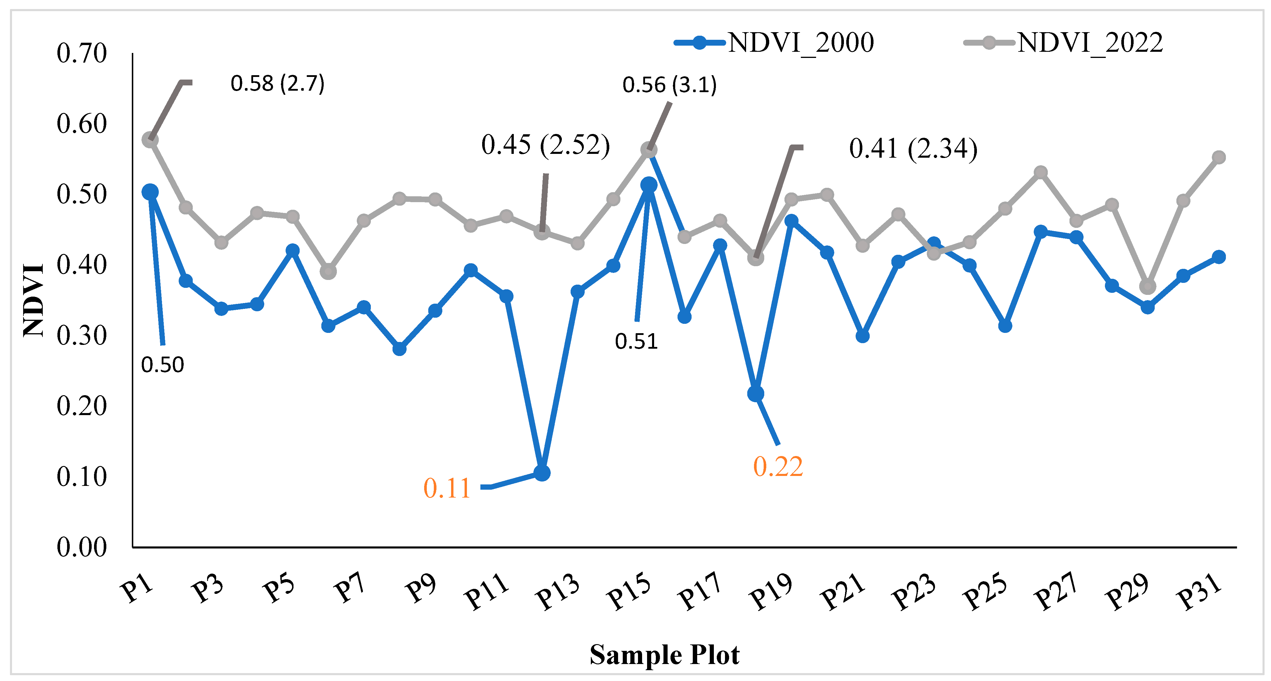
3.1. Comparing the NDVI of 2000 and 2022 of the Lake Complex

We found vast differences in the NDVI between 2000 and 2022 (Figure 2). We found that the NDVI was higher in 2022 (mean = 0.47, SE = 0.0084, SD = 0.0467) than in 2000 (mean = 0.37, SE = 0.0144, SD = 0.0804) (p < 0.00001). The NDVI of 31 sampling plots was compared, which showed that in 2000, Plot 12 had the lowest NDVI (0.11), and Plot 15 had the highest NDVI (0.51), while in 2022, Plot 12 had an NDVI of 0.45 and plant diversity of 2.52 and Plot 15 had an NDVI of 0.56 and plant diversity of 3.1. This relation shows that an increase in the NDVI corresponds with an increase in plant diversity. The NDVI showed a stronger indication of plant diversity in 2022 than in 2000. In 2022, the NDVI ranged from 0.58 to 0.37.

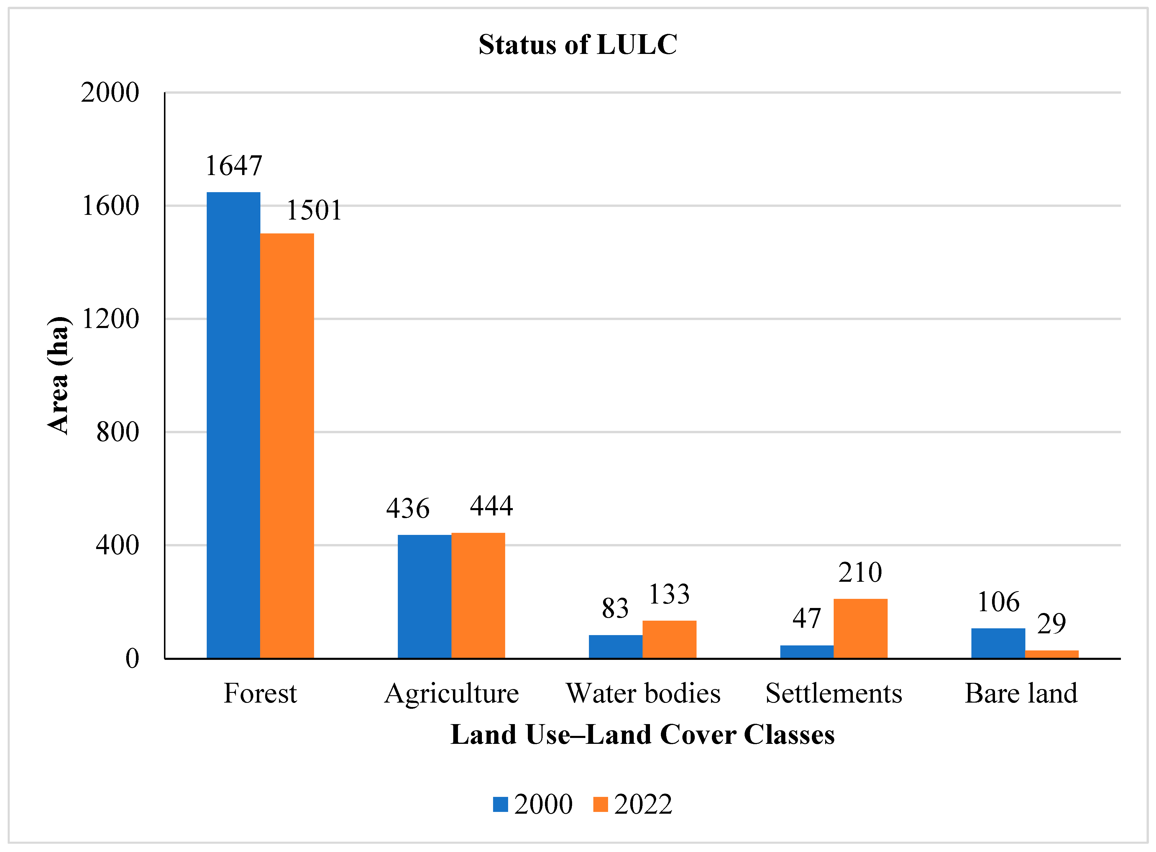
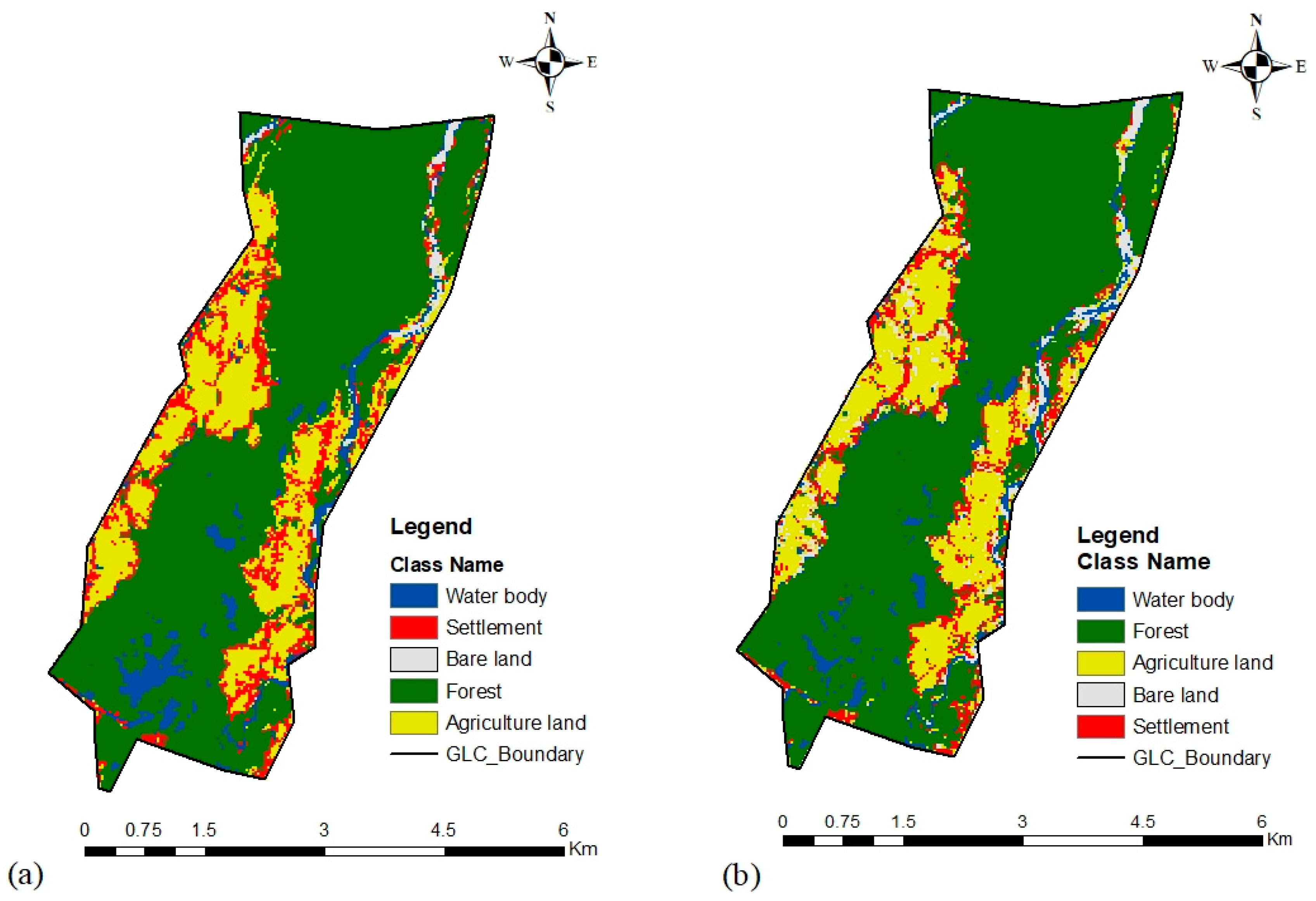
3.2. Land Use and Land Cover Change in the Ghodaghodi Lake Complex

Landsat 7 (ETM+) and Landsat 9 (OLI 2/TIRS 2) images were used for the land use–land cover classification. The Landsat images showed major changes in the forest and agricultural land in the GLC (

Table 1. The change in land use and land cover (LULC) in Ghodaghodi Lake Complex, Nepal, between April and December 2000.

Site	LULC Classes	LULC 2000 (April)		LULC 2000 (December)
		Area (ha)	Area (%)	Area (ha)	Area (%)
1	Forest	1646.78	71.05	1262.53	54.48
2	Agricultural land	435.99	18.81	632.21	27.28
3	Water bodies	82.72	3.57	214.80	9.27
4	Settlement	46.72	2.02	41.24	1.78
5	Bare land	105.53	4.55	166.62	7.19
Grand total		2317.74	100	2317.39	100

,

Table 2. Land use and land cover (LULC) change in Ghodaghodi Lake Complex, Nepal, between April and November 2022.

Site	LULC Classes	LULC 2022 (April)		LULC 2022 (November)
		Area (ha)	Area (%)	Area (ha)	Area (%)
1	Forest	1500.85	64.762	1513.14	65.29
2	Agricultural land	444.28	19.171	431.36	18.61
3	Water bodies	133.31	5.752	116.74	5.04
4	Settlement	210.36	9.077	159.95	6.90
5	Bare land	28.69	1.238	96.53	4.16
Grand total		2317.48	100	2317.72	100

and

Table 3. Current land use and land cover (LULC) change in Ghodaghodi Lake Complex, Nepal, between 2000 (April) and 2022 (April).

Site	LULC Classes	LULC 2000		LULC 2022
		Area (ha)	Area (%)	Area (ha)	Area (%)
1	Forest	1646.78	71.05	1500.85	64.762
2	Agricultural land	435.99	18.81	444.28	19.171
3	Water bodies	82.72	3.57	133.31	5.752
4	Settlement	46.72	2.02	210.36	9.077
5	Bare land	105.53	4.55	28.69	1.238
Grand total		2317.74	100	2317.48	100

). The image classification of April 2000 showed that about 71.05% of the land was covered by forest, the main land cover in the study area, while agriculture occupied 18.81% (Figure 3 and Figure 4). Water bodies, settlements, and bare ground occupied 3.57%, 2.02%, and 4.55%, respectively. In December, about 54.48% of the land was covered by forest; agriculture, water, settlements, and bare land occupied 27.28%, 9.37%, 1.78%, and 7.19%, respectively. Similarly, the image classification of April 2022 shows that forest cover was the dominant land cover (64.76%) (Figure 3 and Figure 5). Likewise, agriculture was still the primary land use covering 19.17%, while water bodies, settlements, and barren land covered around 5.75%, 9.01%, and 1.24%, respectively. In November, about 65.3% of the land was covered by forests; agriculture, water, settlements, and bare ground occupied 18.6%, 5%, 6.9%, and 4.2%, respectively.

Forest cover changed into other land uses and cover from 2000 to 2022 (Table 3). While water bodies were changed into forests of 33 ha, similarly, settlements were converted into forest areas of 10 ha (Figure 6 and Figure 7). In contrast, forest cover was transformed into water bodies, settlements, forests, bare land, and agricultural land of 49 ha, 99 ha, 1357 ha, 7 ha, and 133 ha, respectively (Figure 7). Barren land was converted into forests of 23 ha, and agricultural land was changed into forests of 78 ha (Figure 7).

3.3. Accuracy Assessment of the Classified Map of 2000 and 2022

Accuracy assessment is integral to any classification project. It compares the classified image to another source considered to be accurate or ground truth data [46]. One hundred and fifty ground truth points (fifty from each class) were collected from different land use–land cover classes. The classification was evaluated using Kappa accuracy. Accuracy was 88.67% and 90.67% for the classified map of 2000 (

Table 4. Accuracy Assessment of Classified Map of April 2000.

Class Name	Water Body	Bare Land	Forest	Settlement	Agricultural Land	TU	UA
Water Body	28	1	1	0	0	30	93.33
Bare Land	0	27	0	0	3	30	90
Forest	0	0	28	0	2	30	93.33
Settlement	0	0	1	26	3	30	86.67
Agricultural Land	2	2	2	0	24	30	80
TP	30	30	32	26	32	150	OA = 88.67
PA	93.33	90	87.5	100	75	Kappa = 0.858

TU: total user, TP: total producer, UA: users’ accuracy, PA: producers’ accuracy, OA: overall accuracy.

and

Table 5. Accuracy Assessment of Classified Map of December 2000.

Class Name	Water Body	Bare Land	Forest	Settlement	Agricultural Land	TU	UA
Water Body	26	0	3	1	0	30	86.67
Bare Land	0	26	2	0	2	30	86.67
Forest	0	0	30	0	0	30	100
Settlement	0	1	1	25	3	30	83.33
Agricultural Land	0	0	1	0	29	30	96.67
TP	26	27	37	26	34	150	OA = 90.67
PA	100	96.29	81.08	96.15	85.29	Kappa = 0.883

TU: total user, TP: total producer, UA: users’ accuracy, PA: producers’ accuracy, OA: overall accuracy.

) and 86.00% and 89.33% for 2022 (

Table 6. Accuracy Assessment of Classified Map of April 2022.

Class Name	Water Body	Bare Land	Forest	Settlement	Agricultural Land	TA	UA
Water Body	24	2	3	0	1	30	80
Bare Land	1	21	1	4	3	30	70
Forest	0	0	30	0	0	30	100
Settlement	1	2	0	24	3	30	80
Agricultural Land	0	0	0	0	30	30	100
TP	26	25	34	28	37	150	OA = 86.00
PA	92.3	84	88.23	85.71	81.08	Kappa = 0.825

TU: total user, TP: total producer, UA: users’ accuracy, PA: producers’ accuracy, OA: overall accuracy.

and

Table 7. Accuracy Assessment of Classified Map of November 2022.

Class Name	Water Body	Bare Land	Forest	Settlement	Agricultural Land	TU	UA
Water Body	25	2	3	0	0	30	83.33
Bare Land	0	28	0	0	2	30	93.33
Forest	0	0	30	0	0	30	100
Settlement	0	0	0	23	7	30	76.67
Agricultural Land	0	0	1	1	28	30	93.33
TP	25	30	34	24	37	150	OA = 89.33
PA	100	93.33	88.23	95.83	75.67	Kappa = 0.867

TU: total user, TP: total producer, UA: users’ accuracy, PA: producers’ accuracy, OA: overall accuracy.

).

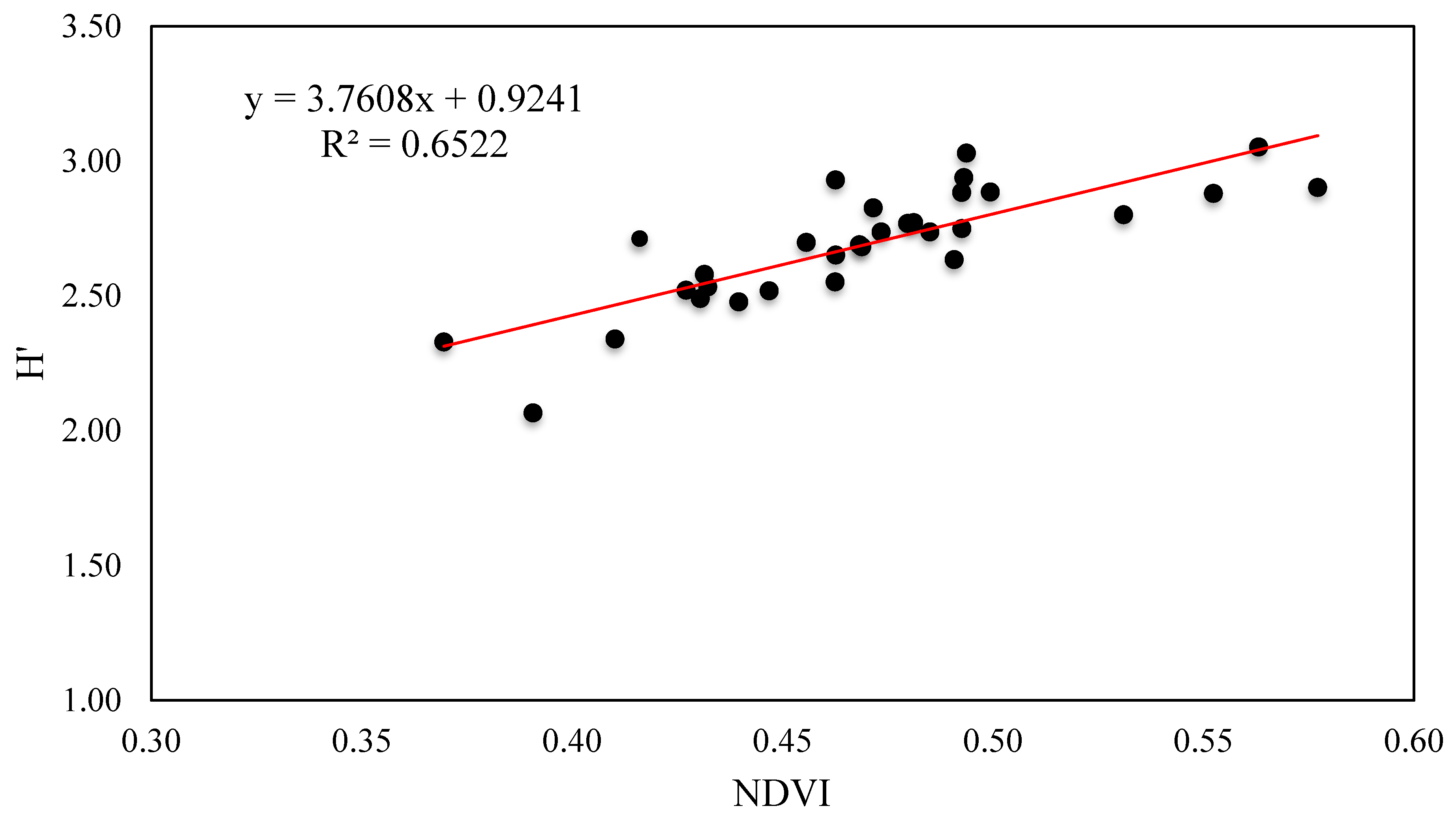
3.4. Diversity Dynamic Depicted Using Remote Sensing

Shannon’s Diversity Index was calculated from the field data. The diversity index ranged from 2.07 to 3.05 (

Table 8. Shannon’s Diversity Index Calculated from sample plots.

Sample Plots	Shannon’s Diversity Index
Plot 1	2.90
Plot 2	2.77
Plot 3	2.58
Plot 4	2.74
Plot 5	2.69
Plot 6	2.07
Plot 7	2.93
Plot 8	3.03
Plot 9	2.75
Plot 10	2.70
Plot 11	2.68
Plot 12	2.52
Plot 13	2.49
Plot 14	2.94
Plot 15	3.05
Plot 16	2.48
Plot 17	2.65
Plot 18	2.34
Plot 19	2.88
Plot 20	2.89
Plot 21	2.52
Plot 22	2.83
Plot 23	2.71
Plot 24	2.53
Plot 25	2.77
Plot 26	2.80
Plot 27	2.55
Plot 28	2.74
Plot 29	2.33
Plot 30	2.63
Plot 31	2.88

). Similarly, Plot 15 and Plot 6 have the highest and lowest diversity index of 3.05 and 2.07, respectively (Table 8). A regression test was performed between Shannon’s Diversity Index and NDVI. We found that plant species diversity depends on NDVI (r = 0.80, p < 0.001). NDVI explained about 65% (r² = 0.6522) of the variety in plant species (Figure 8).

4. Discussion

The results present the change in land cover over the past 22 years. The forest cover decreased by 6.29% over 22 years. Similarly, the agricultural area increased by 0.36%, water bodies increased by 2.18%, settlements increased by 7.06%, and bare land decreased by 3.31%. Although there was a decrease in forest cover, water bodies, primarily impoundments and dugouts, grew.

Khanal [54] found that forest cover decreased by 75%, 70%, 65%, and 64% in 1977, 1990, 1999, and 2008, respectively, in three village development committees (VDCs) of the lake complex (i.e., Darakh, Sadapani, and Ramshikharjhala). The loss in forest cover in the VDC lake complex was highest between 1990 and 1999 [54]. Anthropogenic activities, such as continuous grazing, deforestation, roads, encroachment, and illegal forest product extraction, were the significant causes of forest cover loss [55,56]. Others have also indicated the role of road construction on forest loss [54]. However, forest loss associated with roads is only part of the story. Roads influence vegetative communities [57], fish and wildlife assemblages [58,59,60,61], soil chemistry [62], stream sedimentation [63], stream morphology [64], water quality [65], and benthic macroinvertebrates [63,65]. Khanal [54] found that southern parts suffer more shrinkage of forest cover than northern parts. This notable change in northern forest cover was due to the natural disaster of floods and landslides [54]. The southern plain is dominated by the highly productive Sal (Shorea robusta) forests and has a higher population density than the northern part. Continuous grazing, illicit tree cutting, and encroachment result in more forest cover loss [54]. Forest cover loss was the most intensive between 1990 and 1999 because of the construction of roads [54]. However, the intensity of deforestation was low but still sustained. The active involvement of local communities, ethnic groups, community forest user groups, and youth groups helped to conserve the lake area.

Similarly, the relationship between plant diversity and NDVI was also assessed. We found a strong correlation between the NDVI and plant diversity from this relationship. Chapungu et al. [27] found that the NDVI explained about 62% of the vegetation index. Our results support previous research suggesting that the NDVI can substitute for vegetative species diversity [19,25,27]. Chapungu et al. [27] used the NDVI as a proxy for plant diversity to cover the absence of long-term historical data on plant diversity. Wang et al. [66] presented the linear relationship of NDVI with biomass but a log relationship with vegetation percentage cover. In the case of sparse canopies (crown cover below 60%), the NDVI is more sensitive, while the NDVI is less sensitive to dense canopies (crown cover above 60%) [66]. Mahananda et al. [67] modeled three categories of forest (i.e., evergreen forest, semi-evergreen forest, and deciduous forest) based on the relation between the NDVI and plant species diversity. Around 2000, heavy road expansion resulted in a significant loss in forest cover [54], affecting the NDVI and likely biota [57,60,61,63] and environmental quality [62,63,64,65]. However, in 2022, because of the active involvement of local communities in forest conservation and protection, the NDVI improved. Gould [19] and Levin et al. [25] also present a positive correlation between the NDVI and species richness. Here, the NDVI and plant species diversity correspond with each other.

5. Conclusions

The land use and land cover change map showed less forest area in 2022 than in 2000. There was an increase in water bodies, and most bare lands were converted to forests. The major change in forest cover might be due to various road construction activities, migrants from the surrounding hills, various illegal activities, and factors such as climate change, forest fires, and landslides. Although there has been a decrease in forest cover, the lake complex has more plant diversity than in 2000. This change might be due to the involvement of local people in community forest management. The lake complex was declared a Ramsar site in 2003, bringing international attention to the conservation of wetlands. Remote sensing attributes play an essential role in assessing plant diversity. The strong correlation between the NDVI and vegetation species diversity shows that the NDVI and plant diversity are surrogates for each other. From this relationship, we conclude that an increase in plant diversity corresponds to a rise in the NDVI and vice versa.

References

1. Dimyati, M.; Mizuno, K.; Kobayashi, S.; Kitamura, T. An analysis of land use/cover change in Indonesia. Int. J. Remote Sens. 1996, 17, 931–944. [Google Scholar] [CrossRef]
2. Rawat, J.S.; Kumar, M. Monitoring land use/cover change using remote sensing and GIS techniques: A case study of Hawalbagh block, district Almora, Uttarakhand, India. Egypt. J. Remote Sens. Space Sci. 2015, 18, 77–84. [Google Scholar] [CrossRef] [Green Version]
3. Maitima, J.M.; Mugatha, S.M.; Reid, R.S.; Gachimbi, L.N.; Majule, A.; Lyaruu, H.; Pomery, D.; Mathai, S.; Mugisha, S. The linkages between land use change, land degradation and biodiversity across East Africa. Ajol. Info 2009, 3, 310–325. Available online: https://www.ajol.info/index.php/ajest/article/view/56259 (accessed on 16 August 2022).
4. Anderson, J.T.; Zilli, F.L.; Montalto, L.; Marchese, M.R.; McKinney, M.; Park, Y.L. Sampling and Processing Aquatic and Terrestrial Invertebrates in Wetlands. In Wetland Techniques; Anderson, J.T., Davis, C.A., Eds.; Springer: New York, NY, USA, 2013; Volume 2, pp. 142–195. [Google Scholar]
5. Balcombe, C.K.; Anderson, J.T.; Fortney, R.H.; Kordek, W.S. Wildlife use of mitigation and reference wetlands in West Virginia. Ecol. Eng. 2005, 25, 85–99. [Google Scholar] [CrossRef]
6. Clipp, H.L.; Anderson, J.T. Environmental and anthropogenic factors influencing salamanders in riparian forests: A review. Forests 2014, 5, 2679–2702. [Google Scholar] [CrossRef] [Green Version]
7. Edalgo, J.A.; JT Anderson, J.T. Effects of prebaiting on small mammal trapping success in a Morrow’s honeysuckle–dominated area. J. Wildl. Manag. 2007, 71, 246–250. Available online: https://www.jstor.org/stable/4495169 (accessed on 25 January 2023). [CrossRef]
8. Veselka, W.V.; Anderson, J.T.; Kordek, W.S. Using dual classifications in the development of avian wetlands indices of biological integrity for wetlands in West Virginia, USA. Environ. Monit. Assess. 2010, 164, 533–548. [Google Scholar] [CrossRef]
9. Gingerich, R.T.; Anderson, J.T. Decomposition trends of five plant litter types in mitigated and reference wetlands in West Virginia, USA. Wetlands 2011, 31, 653–662. [Google Scholar] [CrossRef]
10. Gingerich, R.T.; Panaccione, D.G.; Anderson, J.T. The role of fungi and invertebrates in litter decomposition in mitigated and reference wetlands. Limnologica 2015, 54, 23–32. [Google Scholar] [CrossRef] [Green Version]
11. Hedrick, L.B.; Anderson, J.T.; Welsh, S.A.; Lin, L.S. Sedimentation in mountain streams: A review of methods and measurements. Nat. Resour. 2013, 4, 92–104. Available online: https://www.scirp.org/journal/paperinformation.aspx?paperid=29185 (accessed on 25 January 2023). [CrossRef] [Green Version]
12. Petty, J.T.; Gingerich, G.; Anderson, J.T.; Ziemkiewicz, P.F. Ecological function of constructed perennial stream channels on reclaimed surface coal mines. Hydrobiologia 2013, 720, 39–53. [Google Scholar] [CrossRef]
13. Stella, J.C.; Rodriguez-Gonzalez, P.M.; Dufour, S.; Bendix, J. Riparian vegetation research in Mediterranean-climate regions: Common patterns, ecological processes, and considerations for management. Hydrobiologia 2013, 719, 291–315. [Google Scholar] [CrossRef]
14. Vitousek, P.M.; Mooney, H.A.; Lubchenco, J.; Melillo, J.M. Human domination of Earth’s ecosystems. Science 1997, 277, 494–499. [Google Scholar] [CrossRef] [Green Version]
15. Sala, O.E.; Chapin, F.S.; Armesto, J.J.; Berlow, E.; Bloomfield, J.; Dirzo, R.; Huber-Sanwald, E.; Huenneke, L.F.; Jackson, R.B.; Kinzig, A.; et al. Global biodiversity scenarios for the year 2100. Science 2000, 287, 1770–1774. [Google Scholar] [CrossRef] [PubMed]
16. Riebsame, W.E.; Meyer, W.B.; Turner, B.L. Modeling land use and cover as part of global environmental change. Clim. Chang. 1994, 28, 45–64. [Google Scholar] [CrossRef]
17. Cho, M.A.; Mathieu, R.; Asner, G.P.; Naidoo, L.; van Aardt, J.; Ramoelo, A.; Debba, P.; Wessels, K.; Main, R.; Smit, I.P.J.; et al. Mapping tree species composition in South African savannas using an integrated airborne spectral and LiDAR system. Remote Sens. Environ. 2012, 125, 214–226. [Google Scholar] [CrossRef]
18. Hernandez-Stefanoni, J.L.; Gallardo-Cruz, J.A.; Meave, J.A.; Rocchini, D.; Bello-Pineda, J.; López-Martínez, J.O. Modeling α- and β-diversity in a tropical forest from remotely sensed and spatial data. Int. J. Appl. Earth Obs. Geoinf. 2012, 19, 359–368. [Google Scholar] [CrossRef]
19. Gould, W. Remote sensing of vegetation, plant species richness, and regional biodiversity hotspots. Ecol. Appl. 2000, 10, 1861–1870. [Google Scholar] [CrossRef]
20. Parviainen, M.; Luoto, M.; Heikkinen, R. NDVI-Based Productivity and Heterogeneity as Indicators of Plant-Species Richness in Boreal Landscapes. 2010. Available online: https://helda.helsinki.fi/bitstream/handle/10138/233102/ber15-3-301.pdf?sequence=1 (accessed on 25 January 2023).
21. Wood, E.M.; Pidgeon, A.M.; Radeloff, V.C.; Keuler, N.S. Image texture predicts avian density and species richness. PloS ONE 2013, 8, e63211. [Google Scholar] [CrossRef] [Green Version]
22. Madonsela, S.; Cho, M.A.; Ramoelo, A.; Mutanga, O. Remote sensing of species diversity using Landsat 8 spectral variables. ISPRS J. Photogramm. Remote Sens. 2017, 133, 116–127. [Google Scholar] [CrossRef] [Green Version]
23. Pau, S.; Gillespie, T.W.; Wolkovich, E.M. Dissecting NDVI–species richness relationships in Hawaiian dry forests. J. Biogeogr. 2012, 39, 1678–1686. [Google Scholar] [CrossRef]
24. Witman, J.D.; Cusson, M.; Archambault, P.; Pershing, A.J.; Mieszkowska, N. The relation between productivity and species diversity in temperate–arctic marine ecosystems. Ecology 2008, 89, S66–S80. [Google Scholar] [CrossRef] [PubMed] [Green Version]
25. Levin, N.; Shmida, A.; Levanoni, O.; Tamari, H.; Kark, S. Predicting mountain plant richness and rarity from space using satellite-derived vegetation indices. Divers. Distrib. 2007, 13, 692–703. [Google Scholar] [CrossRef]
26. Posse, G.; Cingolani, A.M. A test of the use of NDVI data to predict secondary productivity. Appl. Veg. Sci. 2004, 7, 201–208. [Google Scholar] [CrossRef]
27. Chapungu, L.; Nhamo, L.; Gatti, R.C. Estimating biomass of savanna grasslands as a proxy of carbon stock using multispectral remote sensing. Remote Sens. Appl. Soc. Environ. 2020, 17, 100275. [Google Scholar] [CrossRef]
28. Walter, R.E.; Stoms, D.M.; Estes, J.E.; Cayocca, K.D. Relationships between biological diversity and multi-temporal vegetation index in California. In Proceedings of the American Society for Photogrammetric Engineering and Remote Sensing. American Congress of Surveying and Mapping, Washington, DC, USA, 2–14 August 1992; pp. 562–571. [Google Scholar]
29. Skidmore, A.; Oindo, B.; Said, M. Biodiversity assessment by remote sensing. In Proceedings of the 30th International Symposium on Remote Sensing of the Environment: Information for Risk Management and Sustainable Development, Honolulu, HI, USA, 25–30 July 2003; pp. 10–14. [Google Scholar]
30. Wang, R.; Gamon, J.A.; Cavender-Bares, J.; Townsend, P.A.; Zygielbaum, A.I. The spatial sensitivity of the spectral diversity–biodiversity relationship: An experimental test in a prairie grassland. Ecol. Appl. 2018, 28, 541–556. [Google Scholar] [CrossRef] [Green Version]
31. Pouteau, R.; Gillespie, T.W.; Birnbaum, P. Predicting tropical tree species richness from normalized difference vegetation index time series: The devil is not in the detail. Remote Sens. 2018, 10, 698. [Google Scholar] [CrossRef] [Green Version]
32. Chitale, V.S.; Behera, M.D.; Roy, P.S. Deciphering plant richness using satellite remote sensing: A study from three biodiversity hotspots. Biodivers. Conserv. 2019, 28, 2183–2196. [Google Scholar] [CrossRef]
33. Jones, H.G.; Vaughan, R.A. Remote Sensing of Vegetation: Principles, Techniques, and Applications; Oxford University Press: Oxford, UK, 2010. [Google Scholar]
34. Mpandeli, S.; Nhamo, L.; Moeletsi, M.; Masupha, T.; Magidi, J.; Tshikolomo, K.; Liphadzi, S.; Naidoo, D.; Mabhaudhi, T. Assessing climate change and adaptive capacity at local scale using observed and remotely sensed data. Weather. Clim. Extrem. 2019, 26, 100240. [Google Scholar] [CrossRef]
35. Matsushita, B.; Yang, W.; Chen, J.; Onda, Y.; Qiu, G. Sensitivity of the enhanced vegetation index (EVI) and normalized difference vegetation index (NDVI) to topographic effects: A case study in high-density cypress forest. Sensors 2007, 7, 2636–2651. [Google Scholar] [CrossRef] [PubMed] [Green Version]
36. Lamsal, P.; Atreya, K.; Ghosh, M.K.; Pant, K.P. Effects of population, land cover change, and climatic variability on wetland resource degradation in a Ramsar listed Ghodaghodi Lake Complex, Nepal. Environ. Monit. Assess. 2019, 191, 1–16. [Google Scholar] [CrossRef] [PubMed]
37. Siwakoti, M.; Karki, J.B. Conservation status of Ramsar sites of Nepal Tarai: An overview. Bot. Orient. J. Plant Sci. 2009, 6, 76–84. [Google Scholar] [CrossRef]
38. Lamsal, P.; Pant, K.P.; Kumar, L.; Atreya, K.; Atangana, A.R.; Bisht, I.; Chistoserdov, A.; De, P.; Escalante, R.; Vergara, P.M. Diversity, uses, and threats in the GhodaghodiLake complex, a Ramsar site in western lowland Nepal. Int. Sch. Res. Not. 2014. [Google Scholar] [CrossRef]
39. IUCN. A Review of the Status and Threats to Wetlands in Nepal; IUCN Nepal: Kathmandu, Nepal, 2004. [Google Scholar]
40. Dnpwc, B. Conserving Biodiversity and Delivering Ecosystem Services at Important Bird Areas in Nepal; Birdlife International: Cambridge, UK, 2012. [Google Scholar]
41. Sah, J.P.; Heinen, J.T. Wetland resource use and conservation attitudes among indigenous and migrant peoples in Ghodaghodi Lake area, Nepal. Environ. Conserv. 2001, 28, 345–356. [Google Scholar] [CrossRef] [Green Version]
42. Dof. Community Forest Inventory Guideline; Department of Forest: Kathmandu, Nepal, 2004. [Google Scholar]
43. Rahman MT, U.; Tabassum, F.; Rasheduzzaman, M.; Saba, H.; Sarkar, L.; Ferdous, J.; Islam, A.Z. Temporal dynamics of land use/land cover change and its prediction using CA-ANN model for southwestern coastal Bangladesh. Environ. Monit. Assess. 2017, 189, 565. [Google Scholar] [CrossRef]
44. Bhatti, S.S.; Tripathi, N.K. Built-up area extraction using Landsat 8 OLI imagery. GIScience Remote Sens. 2014, 51, 445–467. [Google Scholar] [CrossRef] [Green Version]
45. Olaniyi, O.; Hlengwa, D.; Anderson, J.T. Assessing the driving forces of Guinea savanna transition using geospatial technology and machine learning in Old Oyo National Park, Nigeria. Geocarto Int. 2023, 37, 17242–17259. [Google Scholar] [CrossRef]
46. Didelija, M.; Kulo, N.; Mulahusić, A.; Tuno, N.; Topoljak, J. Segmentation scale parameter influence on the accuracy of detecting illegal landfills on satellite imagery. A case study for Novo Sarajevo. Ecol. Inform. 2022, 70, 101755. [Google Scholar] [CrossRef]
47. Cohen, J. Weighted kappa: Nominal scale agreement provision for scaled disagreement or partial credit. Psychol. Bull. 1968, 70, 213–220. [Google Scholar] [CrossRef]
48. FAO. Forest Resources Assessment 1990; Global Synthesis FAO: Rome, Italy, 1995; Available online: http://www.fao.org/docrep/007/v5695e/v5695e00.htm (accessed on 25 January 2023).
49. Kumar, K.S.; Bhaskar, P.U.; Padmakumari, K. Estimation of land surface temperature to study urban heat island effect using Landsat ETM+ image. Int. J. Eng. Sci. Technol. 2012, 4, 771–778. [Google Scholar]
50. Weier, J.; Herring, D. Measuring Vegetation (ndvi & evi). NASA Earth Obs. 2000, 20. Available online: https://earthobservatory.nasa.gov/features/MeasuringVegetation (accessed on 16 August 2022).
51. Li, F.; Chen, W.; Zeng, Y.; Zhao, Q.; Wu, B. Improving Estimates of Grassland Fractional Vegetation Cover Based on a Pixel Dichotomy Model: A Case Study in Inner Mongolia, China. Remote Sens. 2014, 6, 4705–4722. [Google Scholar] [CrossRef] [Green Version]
52. Kent, M.; Coker, P. Vegetation Description and Analysis: A Practical Approach; John Wiley and Sons: New York, NY, USA, 1992; p. 363. [Google Scholar]
53. Shannon, C.E. A mathematical theory of communication. Bell Syst. Tech. J. 1948, 27, 379–423. [Google Scholar] [CrossRef] [Green Version]
54. Khanal, S. Change assessment of forest cover in Ghodaghodi lake area in Kailali district of Nepal. Banko Janakari 2009, 19, 15–19. [Google Scholar] [CrossRef] [Green Version]
55. Bhandari, B. Wise use of wetlands in Nepal. Banko Janakari 2009, 19, 10–17. [Google Scholar] [CrossRef]
56. Diwakar, J.; Barjracharya, S.; Yadav, U. Ecological study of Ghodaghodi lake. Banko Janakari 2009, 19, 18–23. [Google Scholar] [CrossRef] [Green Version]
57. Rentch, J.S.; Fortney, R.H.; Stephenson, S.L.; Adams, H.S.; Grafton, W.N.; Anderson, J.T. Vegetation-site relationships of roadside plant communities in West Virginia USA. J. Appl. Ecol. 2005, 42, 129–138. [Google Scholar] [CrossRef]
58. Poplar-Jeffers, I.O.; Petty, J.T.; Anderson, J.T.; Kite, J.S.; Strager, M.P.; Fortney, R.H. Culvert replacement and stream habitat restoration: Implications from brook trout management in an Appalachian watershed USA. Restor. Ecol. 2009, 17, 404–413. [Google Scholar] [CrossRef]
59. Ward, R.L.; Anderson, J.T.; Petty, J.T. Effects of road crossings on stream and streamside salamanders. J. Wildl. Manag. 2008, 72, 760–771. [Google Scholar] [CrossRef]
60. Vance, J.A.; Angus, N.B.; Anderson, J.T. Effects of bridge construction on songbirds and small mammals at Blennerhassett Island, Ohio River, USA. Environ. Monit. Assess. 2013, 185, 7739–7748. [Google Scholar] [CrossRef] [PubMed]
61. Vance, J.A.; Angus, N.B.; Anderson, J.T. Riparian and riverine wildlife response to a newly created bridge crossing. Nat. Resour. 2012, 3, 213–228. [Google Scholar] [CrossRef] [Green Version]
62. Vance, J.A.; Angus, N.B.; Rentch, J.S.; Anderson, J.T. Vegetation and soil parameters at an island bridge crossing. Castanea 2014, 79, 59–73. [Google Scholar] [CrossRef] [PubMed]
63. Hedrick, L.B.; SA Welsh, S.A.; Anderson, J.T. Effects of highway construction on sediment and benthic macroinvertebrates in two tributaries of the Lost River, West Virginia. J. Freshw. Ecol. 2007, 22, 561–569. [Google Scholar] [CrossRef] [Green Version]
64. Hedrick, L.B.; Welsh, S.A.; Anderson, J.T. Influences of high-flow events on a stream channel altered by construction of a highway bridge: A case study. Northeast. Nat. 2009, 16, 375–394. [Google Scholar] [CrossRef]
65. Chen, Y.; Viadero, R.C., Jr.; Wei, X.; Hedrick, L.B.; Welsh, S.A.; Anderson, J.T.; Lin, L. Effects of highway construction on stream water quality and macroinvertebrate condition in a Mid-Atlantic highlands watershed, USA. J. Environ. Qual. 2009, 38, 1672–1682. [Google Scholar] [CrossRef] [PubMed] [Green Version]
66. Wang, R.; Gamon, J.A.; Montgomery, R.A.; Townsend, P.A.; Zygielbaum, A.I.; Bitan, K.; Tilman, D.; Cavender-Bares, J. Seasonal Variation in the NDVI–Species Richness Relationship in a Prairie Grassland Experiment (Cedar Creek). Remote Sens. 2016, 8, 128. [Google Scholar] [CrossRef] [Green Version]
67. Mahanand, S.; Behera, M.D.; Roy, P.S. Rapid assessment of plant diversity using MODIS biophysical proxies. J. Environ. Manag. 2022, 311, 114778. [Google Scholar] [CrossRef]
Figure 1. Location of Ghodaghodi Lake Complex (GLC) in the map of Nepal and its land use.
Forests 14 00529 g001
Figure 2. Comparing normalized difference vegetation index (NDVI) between 2000 and 2022 in Ghodaghodi Lake Complex, Nepal.
Forests 14 00529 g002
Figure 3. Histogram of land use and land cover (LULC) change in Ghodaghodi Lake Complex (GLC), Nepal, 2000 (April) and 2022 (April).
Forests 14 00529 g003
Figure 4. Classified land use and land cover (LULC) map of Ghodaghodi Lake Complex, Nepal, 2000 data. (a) LULC map in April, (b) LULC map in December.
Forests 14 00529 g004
Figure 5. Classified land use and land cover (LULC) map of Ghodaghodi Lake Complex, Nepal, 2022 data. (a) LULC map in April, (b) LULC map in November.
Forests 14 00529 g005
Figure 6. Change detection of land use and land cover (LULC) change in Ghodaghodi Lake Complex, Nepal, between 2000 (April) and 2022 (April).
Forests 14 00529 g006
Figure 7. Histogram showing changes in land use cover between 2000 and 2022 in the Ghodaghodi Lake Complex, Nepal.
Forests 14 00529 g007
Figure 8. Relationship between normalized difference vegetation index (NDVI) and Shannon–Wiener diversity index (H’) for vegetation in Ghodaghodi Lake Complex, Nepal.
Forests 14 00529 g008