
Number Preference as a Source of Measurement Error in the U.S. National Forest Inventory

USDA Forest Service, Southern Research Station, Knoxville, TN 37919, USA
Forests 2023, 14(3), 459; https://doi.org/10.3390/f14030459
Submission received: 2 February 2023
/
Revised: 20 February 2023
/
Accepted: 21 February 2023
/
Published: 23 February 2023
(This article belongs to the Section Forest Inventory, Modeling and Remote Sensing)
Abstract
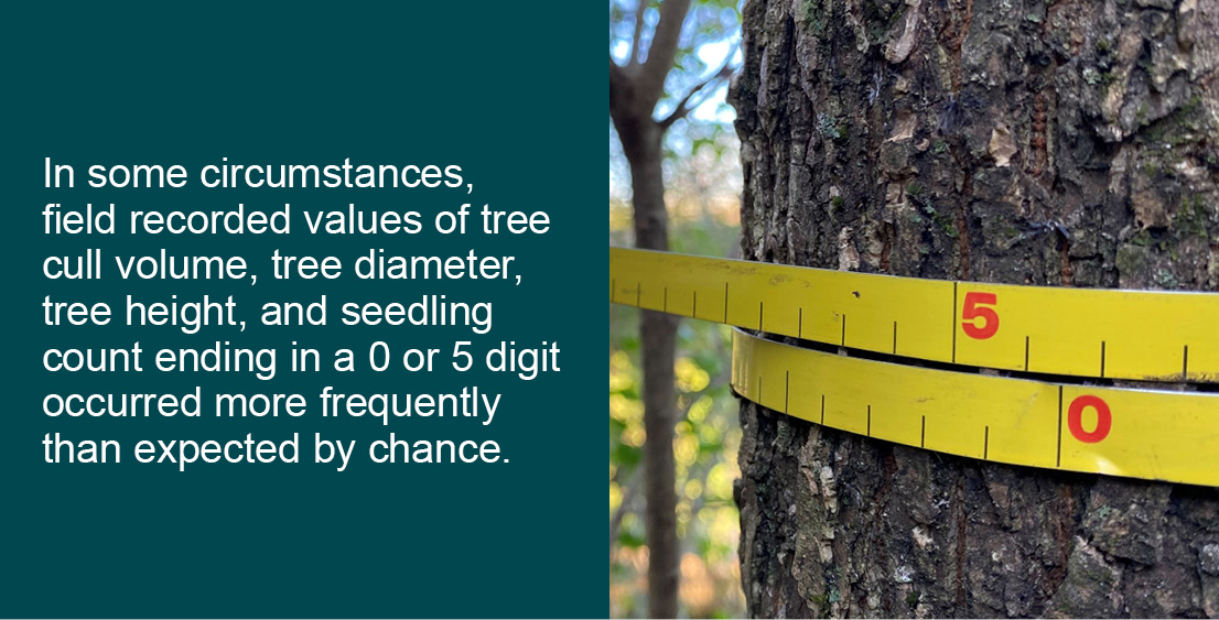
:Number preference, i.e., the human tendency to gravitate toward or away from specific numbers, is a potential source of measurement error in forest inventory. Identifying its presence is an important step to ensure unbiased results. This study evaluated U.S. national forest inventory data for number preference and identified factors that influence the proportion of tree cull volume, tree diameter, tree height, and seedling count observations ending with the digit zero or five (ED0,5) and seedling count observations that were multiples of four (M4). Two-sided hypothesis tests determined that ED0,5 occurred significantly more frequently than expected by chance for all metrics tested, though not in every inventory region of the country nor to the same degree. Consistently, tree-level ED0,5 was more likely when metrics were estimated visually rather than measured instrumentally. Logistic regression indicated that the effect of species class, species type, tree status, treetop status, and stem size on tree-level ED0,5 and the effect of plot-level water depth on seedling count ED0,5 also varied by region. Though the effect was small, findings suggest that some inventory regions may be employing an approved multiplicative shortcut that results in a greater-than-expected proportion of M4 observations among seedling counts.

1. Introduction
The goal of forest inventory is to accurately characterize forest attributes and do so with reasonable precision. As such, estimates of forest attributes are typically presented in terms of a confidence interval
where is the attribute mean, is the standard error of the mean, and c is a constant determined by the desired level of confidence. For any given level of confidence, the width of the confidence interval is determined by the error, or variability, in the sample. In general, there are three sources of error for forest inventories: sampling error, modeling error, and measurement error [1]. Emphasis usually focuses on sampling error, with some attention given to modeling error. Measurement error typically receives little attention because it is commonly assumed that observations are made without any error or with an error that is small and inconsequential when compared to other sources of error [2]. In reality, observational errors are unavoidable and may be quite severe. Their presence can produce biased and imprecise estimates and mask true relationships [3,4].
Common sources of measurement error in a forest inventory include uncalibrated or faulty equipment, negligent record keeping, and lax or improper field techniques. A less cited source of measurement error occurs when data are coarsened by rounding or other approximation. Number preference (NP), i.e., the human tendency to gravitate toward or away from specific numbers [5], is a type of data coarsening. NP occurs in a variety of circumstances, ranging from baseball players modifying their at-bat strategy to end the season with a batting average over 0.300 [6] to diners leaving gratuities in whole-dollar amounts or in amounts that make the total bill a whole-dollar amount [7]. Other examples of NP have been observed in marathon run times [8], economic and financial environments [9,10], human dimension surveys and behavioral studies [6,11,12,13], and wildlife sampling [14]. The phenomenon occurs not only when individuals self-report metrics such as income [15] but also when instrumentation is used for direct measurements, e.g., blood pressures [16], carcinoma sizes [17], and fish lengths [18].
NP, sometimes referred to as digit preference [19], leads to an excessive grouping together, or heaps, of observations at specific values. For example, consider a survey asking respondents how many days they spent vacationing last year, with responses showing an unusually high frequency at 14 days. Though some respondents likely spent exactly two weeks vacationing, others may have spent a day or two more (or less) on holiday and simply rounded to 14 when completing the survey. Datasets such as this may be inaccurate and biased, though not necessarily so, and can lead to erroneous conclusions because means, variances, and percentiles are all affected [15]. Therefore, examining data for NP is recommended for the data processing and quality control steps of forest inventory to ensure accurate characterization. To that end, the objective of this work was to evaluate the extent of NP in data collected by the U.S. national forest inventory and identify which factors, if any, influence the propensity for NP. In this study, the numbers of preference are those ending with the digit zero or five (NP0,5) and those that are a multiple of four (NP4).
2. Materials and Methods
The data used in this study were collected by the Forest Inventory and Analysis (FIA) program of the U.S. Department of Agriculture, Forest Service (Forest Service). FIA inventory plots are located across the U.S. quasi-systematically with a baseline sampling intensity of 1 plot per 2428 ha [20]. Some states, national forests, and other areas are sampled at intensities two or three times that of the baseline. Each plot consists of four 7.32 m fixed-radius subplots on which trees ≥ 12.7 cm in diameter are measured. Observations on trees < 12.7 cm in diameter are made on a 2.07 m fixed-radius microplot within each subplot. The cluster of subplots is arranged with one central subplot, and three other subplots located 36.58 m from the central subplot at azimuths of 0°, 120°, and 240°. Each plot is monumented, georeferenced, and measured on an ongoing basis once every 5–10 years.
When plots are partially forested or straddle heterogeneous forest conditions, they are subdivided by a procedure known as condition mapping [20]. Multiple conditions are classified on the basis of reserved status, owner group, forest type, stand size class, regeneration status, and tree density [21]. Several ancillary attributes are used to further describe the condition classes but are not used to delineate new classes. Any number of condition classes may be recorded for each plot.
NP0,5 was evaluated for three tree-level attributes: rotten/missing cull volume, diameter, and actual height. NP0,5 and NP4 were evaluated for the microplot metric seedling tree count. Rotten/missing cull volume (cull) is the estimated percentage of tree volume that is rotten or missing. Cull is visually estimated and recorded to the nearest 1%. The diameter of timberland tree species is recorded at breast height (d.b.h.), typically 1.37 m above the ground line on the uphill side of the tree. For woodland (mostly multi-stemmed) species, diameter is recorded at the stem root collar (d.r.c.) or groundline, whichever is higher. Diameter is measured instrumentally unless circumstances warrant otherwise and recorded to the nearest 0.254 cm. Actual height (height) is the tree length from ground level to the highest remaining portion of the tree still present and attached to the bole. Height is measured instrumentally unless circumstances warrant otherwise and recorded to the nearest 30.48 cm. The seedling count is the number of live trees with a diameter < 2.54 cm present on the microplot. To qualify for counting, conifer (softwood) seedlings must be at least 15.24 cm tall, and hardwood seedlings must be at least 30.48 cm tall. Seedlings are tallied by species and condition class up to a count of five and estimated beyond that.
Tree-, condition-, and subplot-level data for the most recent available inventory year of all states except Hawaii were included in the analysis (Figure 1). Data were collected with protocols outlined in FIA field guide versions 7–9 [21]. Only plots of the baseline sampling frame were included. The number of tree and seedling count observations available for analysis varied by region and ranged from <1000 to >235,000 (Table 1). All data are available to the public through the FIA online database [22] and were downloaded during the first week of July and the second week of August 2022.
To test for NP0,5, each cull, diameter, height, and seedling count observation was assigned its end digit (EDi). For example, the end digits of numbers 7, 19, and 23.6 were 7, 9, and 6, respectively. End-digit assignments for diameter and height were based on the U.S. customary units of measure employed by FIA (inches and feet, respectively). The proportion of observations ending in zero or five () was estimated for each attribute with a logistic regression model. Cull values = 0%, seedling counts < 11, and seedling counts observed in condition classes with a stocking value < 10, i.e., non-stocked conditions, were not included. Confidence intervals for (α = 0.01) were computed with a Wald-type interval on the log odds scale and transformed to the probability scale. Analyses were completed with R [23] packages survey [24] and srvyr [25]. Tree and seedling count observations were treated as being clustered on plots by designating plot identification number as the primary sampling unit, i.e., cluster variable, in the survey design specification. Estimations of were made for each attribute by region: Interior West (IW), Northern, Pacific Northwest (PNW), and Southern (Figure 1). In the absence of NP, the digits i = 0, 1, …, 9 were expected to occur with equal frequency ( = 0.1) at the end of a number. Therefore, the null hypothesis for NP0,5 was
The null hypothesis was rejected if the 99% confidence interval for did not include 0.2.
The test for NP4 was limited to seedling count and warranted by a recommended tally shortcut: when seedlings are distributed evenly on a microplot, inventory crew members may estimate the total count by multiplying the number of seedlings on one-quarter of the microplot by four [21]. Therefore, all seedling counts > 10 were categorized as either a multiple of four (M4) or not a multiple of four. Procedures used to estimate were repeated to estimate the proportion of M4 seedling counts (). Seedling counts made on microplots with more than one condition class were excluded. The proportion of M4 numbers from 11 to 999 (the maximum seedling count allowed) is approximately 0.25. Thus, the null hypothesis for NP4 was
The null hypothesis was rejected if the 99% confidence interval for did not include 0.25.
Multivariate logistic regression [26] was used to identify factors associated with ED0,5 and M4. Four tree-level attributes were included as potential predictors of cull ED0,5: species group (hardwood, softwood), species type (timberland, woodland), tree status (live, standing dead), and treetop status (intact, broken/missing). Five tree-level attributes were included as potential predictors of diameter ED0,5: diameter point (at breast height, above breast height, below breast height, root collar), method (measured, estimated, different location), species group, stem size (sapling, tree), and tree status. Five tree-level attributes were included as potential predictors of height ED0,5: method (measured, estimated), species group, species type, stem size, and tree status. A detailed description of these factors is provided in Table S1. Seven condition-level attributes and one subplot-level attribute were included as potential influencers of seedling count ED0,5 and M4: stand size (small, medium, large), stand origin (natural, artificial), disturbance (undisturbed, disturbed), treatment (untreated, treated), depth of water or snow on the subplot (<3 cm, 3–30 cm, >30 cm), owner group (Forest Service, other federal, state/local government, private), physiography (mesic, hydric, xeric), and slope (0%–155%). A detailed description of these factors is provided in Table S2. Some factors were omitted in some regional regressions due to inadequate sample sizes.
For the ED0,5 regression, an end digit of zero or five was considered a success (S = 1), and any other end digit a failure (S = 0). For the M4 regression, multiples of four were considered successes (S = 1), and other values were considered failures (S = 0). The probability that S = 1 was modeled for each attribute by region in the linear form as
where parameter βi refers to the effect of attribute xi on the log odds that S = 1, controlling for all other attributes. Dichotomous (0/1) dummy variables were used to represent the categorical attributes. Parameters were estimated with a logit link function under a quasibinomial distribution with R [23] packages survey [24] and srvyr [25]. Tree and seedling count observations were treated as being clustered on plots by designating plot identification number as the primary sampling unit, i.e., cluster variable, in the survey design specification.
3. Results
3.1. Rotten/Missing Cull Volume
Severe heaping at values ending in zero or five was evident in the frequency distribution of cull observations (Figure 2). The null hypothesis (Equation (1)) was rejected (α = 0.01) for all four FIA regions (Table 1). Factors influencing ED0,5 (α = 0.01) varied among regions (Table 2). All other attributes being equal, the odds for ED0,5 was significantly greater for woodland tree species in the Southern region and trees with broken/missing tops in the IW, Northern, and Southern regions than for timberland tree species and trees with intact tops, respectively. In contrast, the odds for ED0,5 was significantly less for softwood trees than hardwood trees in the IW and Southern regions. Tree status was the only significant attribute associated with ED0,5 in the PNW region. There, ED0,5 was less likely for standing dead trees than live trees; the opposite was true in the IW and Southern regions.
3.2. Diameter
Though heaping at values ending in zero or five was not readily apparent in the frequency distribution of tree diameters (Figure 3), the null hypothesis (Equation (1)) was rejected (α = 0.01) for all four FIA regions (Table 1); however, no was greater than 0.22 in any region. The method by which the diameter was acquired and the size of the tree being measured were the only significant (α = 0.01) predictors of ED0,5 (Table 3). This was the case in all regions except the IW, for which no attribute proved to be significant. All other attributes being equal, estimated diameters were 1.5 to 2.1 times more likely to exhibit ED0,5 than measured diameters, and diameters < 12.7 cm (saplings) were 9% less likely to exhibit ED0,5 than diameters ≥ 12.7 cm.
3.3. Actual Height
Some heaping at values ending in zero or five was apparent in the frequency distribution of height (Figure 4). The null hypothesis (Equation (1)) was rejected (α = 0.01) for all four FIA regions, though was no greater than 0.24 in any one region (Table 1). All of the attributes included as potential predictors of ED0,5 were significant (α = 0.01) in at least one region (Table 4). Similar to diameter, estimated heights were more likely to exhibit ED0,5 than measured heights, but only in the Northern and PNW regions. Heights of softwood trees in the Northern and PNW regions were less likely to exhibit ED0,5 than hardwood trees. In addition, less likely to exhibit ED05 were heights of woodland species in the IW region and heights of standing dead trees in the Northern region. ED0,5 was more likely to be exhibited among heights of trees ≥ 12.7 cm d.b.h./d.r.c. than among heights of smaller (sapling-sized) trees in the Northern and Southern regions; this is the opposite of what was observed for diameter.
3.4. Seedling Count
Some heaping at values ending in zero or five was apparent in the frequency distribution of seedling count (Figure 5). The null hypothesis (Equation (1)) was rejected (α = 0.01) for the IW region only (Table 1). Disturbance and water class were the only qualitative attributes significantly (α = 0.01) associated with ED0,5 and only in the Southern region (Table 5). There, seedling counts made on disturbed subplots or subplots with ≥3 cm of standing water were 1.5 and 2.1 times more likely to exhibit ED0,5, respectively, than those made on undisturbed subplots or subplots with <3 cm of standing water. In addition, in the Southern region, a 1% increase in slope was estimated to have a multiplicative effect of 0.98 on the odds of seedling count ED0,5.
The single condition class requirement applied to the analysis of M4 had a minimal effect on the data, reducing the number of observations by two in the IW region, three in the PNW region, and four in both the Northern and Southern regions. Among the remaining observations, was significantly (α = 0.01) greater than expected (Equation (2)) in the Northern (0.28 ± 0.02) and Southern regions (0.30 ± 0.03) but not in the IW (0.26 ± 0.05) and PNW (0.25 ± 0.04) regions. Though small, the regional differences among suggest that the multiplication-by-four shortcut to estimate seedling count may be employed more often in the Northern and Southern regions than in the IW and PNW regions. Stand size was the only attribute significantly (α = 0.01) associated with ED4 and only in the PNW region (Table 6), where all other attributes being equal, M4 seedling counts made in medium-sized stands were 81% less likely than those made in small-sized stands.
4. Discussion
4.1. Considerations for Data Quality Control
The application of statistical tools to minimize uncertainty and ensure that data are of sufficient quality is part of the Quality Assurance (QA) program implemented by the U.S. national forest inventory [27]. Evaluating measurement errors resulting from NP is a way to identify aspects of data collection that need adjusting and for which training should be improved. In general, results suggest that emphasized training is needed for attributes that are visually estimated either by design or because of special circumstances. This evaluation also suggests that cull may be measured best in 5% increments rather than 1% increments. Doing so would remove unwarranted expectations of precision and might speed up data collection. Modifying standard operating procedures, however, should be performed carefully and with a thorough evaluation of the consequences, especially when data are used for long-term monitoring because changes may introduce bias and disrupt trend analyses [4]. Moreover, the statistically significant presence of minimal heaping, e.g., in the case of diameter and height, may not translate to practical significance in subsequent analyses and applications.
Without evidence that seedlings are distributed more homogeneously across the forest floor in the eastern U.S. than in the western U.S., the observation that the multiplication-by-four shortcut to estimate seedling count may be employed more often in the Northern and Southern regions than in the IW and PNW regions may indicate a difference in training among the regions. Furthermore, that was closest to the expected value in the PNW region may be related to the fact that the shortcut is not stated explicitly in the PNW variant [28,29] of the national data collection manual [21].
4.2. Source of Number Preference
Identifying the reason for heaped data is complex because NP is the result of multiple interacting factors. These include the inherent nature of numbers, human psychology and behavior, and the circumstances of measurement. Unless there is a context for a different set of numbers, e.g., 7, 14, and 21 for days spent vacationing, multiples of zero and five are typically preferred [30]. This is largely due to the decimal place-value system, which makes factors of 10 and their halves convenient and readily understandable [5].
One theory behind NP is the behavior known as satisficing, i.e., providing a number that is considered “good enough”. Giving a satisficed answer requires less knowledge and less effort than providing a precise answer. Krosnick [31], as cited in [10] (p. 191), expressed the probability of satisficing as
In this model, task difficulty is a measure of the complexity required to retrieve information (from memory or elsewhere) in order to answer a question. Ability is a measure of cognitive competence and experience with the topic under questioning. Motivation is a measure of how important a precise answer is perceived to be and the respondent’s interest in the topic of inquiry. When motivation and/or ability are high, the tendency for satisficing decreases. When difficulty is high, the tendency increases. Though initially proposed in the context of economic decision making, this model is applicable to forest inventory where task difficulty can be described primarily by forest conditions, ability by field personnel characteristics, and motivation by both forest conditions and personnel disposition, in addition to business expectations.
4.2.1. Task Difficulty
The difficulty of conducting a forest inventory is largely governed by the size, form, and condition of trees, both individually and collectively. For example, McRoberts and others [32] observed greater discrepancies among repeated diameter measurements on larger trees than on smaller trees, and Westfall [33] found more frequent differences in cull proportions on trees that were minimally or mostly culled than on trees that were moderately cull. In this study, traits for which task difficulty, and thus NP, were expected to be greatest were
- Cull measurements of hardwood species due to their deliquescent crown forms [33];
- Cull measurements of trees with broken/missing tops due to their irregular crown form;
- Diameters measured above breast height or at root collar because of the awkward positioning observers must achieve in order to obtain the measurements, i.e., stretching high or crouching low;
- Heights of hardwood species due to their deliquescent crown form [33];
- Heights of trees greater than sapling size due to poorer lines of sight for the observer because the treetops are taller and farther from the observer and potentially obscured by understory vegetation;
- Seedling counts in small-sized stands and disturbed conditions due to dense understory vegetation;
- Seedling counts in conditions where the forest floor is obscured due to snow cover or water; and
- Seedling counts on steep slopes because of the precarious stance observers must maintain in order to obtain the counts.
With the exception of numbers 3, 7, and 9, these expectations were met, though not necessarily in every region. Results were most consistent with expectation 2, which was met in three of the four regions (IW, Northern, Southern). Expectation 1 was met in two regions (IW, South), as were expectations 4 (Northern, PNW) and 5 (Northern, Southern). Expectation 6 was met solely in the IW region, and expectation 8 was met only for ED0,5 in the Southern region.
In addition to tree size, form, and condition, accurate assessments based solely on personal judgment are more difficult to make than assessments with little to no room for individual judgment [32]. Thus, was expected to be greater for cull than for diameter and height, except in instances when the latter two were estimated. This was indeed the case: ED0,5 among all cull observations was 1.5–5.3 times more likely than ED0,5 among all diameter observations and 1.2–2.7 times more likely than ED0,5 among all height observations. Likewise, ED0,5 was 1.2–2.1 times more likely to occur when diameter and height were estimated visually than when they were measured instrumentally. Fortunately, estimations of diameter and height are relatively rare. In this study, diameter estimation occurred for <2% of the trees observed in any region. Estimated heights were also relatively rare in the IW and Southern regions (≤6% per region) but less so in the Northern and PNW regions (26% in each region).
4.2.2. Motivation and Ability
Neither motivation nor ability was evaluated in this study, but steps could be taken to do so in the future. Of the two, ability is more easily quantified. Practical experience increases familiarity with forest inventory methods and provides exposure to rare and unusual situations by which personal judgments can be refined. Assuming a positive correlation with experience, ability could be measured as the number of years employed or the cumulative number of plots completed.
Observers rarely seek to purposefully bias results [36]; therefore, NP may emerge unintentionally due to diminished motivation caused by mental and physical fatigue [37,38]. Forest inventory crew members are exposed to multiple sources of fatigue during the course of an inventory, including steep topography, dense stands, lengthy traverses, long commutes, and early waking hours. Quantifying these factors as surrogates for motivation could be accomplished at the plot or worker level. Because the inclination for NP varies from person to person, factors such as steps taken, heart rate, and hours slept might correlate more strongly with fatigue and motivation than factors such as slope, trees per hectare, and kilometers driven. Nevertheless, plot-related factors may be the better alternative because worker-specific factors are highly individualized, context-specific, and ideally kept private [39].
In addition to plot-related factors, decreased motivation may be caused by weather conditions. In a meta-analysis of temperature effects on worker performance, Pilcher and others [40] reported that performance declined by >7% at hot experimental temperatures ≥ 26.67 °C, wet bulb globe temperature (WBGT), and cold experimental temperatures < 18.3 °C. Productivity was especially affected (~14% decline) at the hottest experimental temperatures (≥32.22 °C WBGT) and coldest experimental temperatures (<10 °C). The length of exposure at higher or lower temperatures prior to and during the task also affected performance. Although Bowen and others [39] did not find a decrease in performance due to high temperatures during forest harvest operations in New Zealand, workers reported that the work felt harder when temperatures were higher (summertime vs. wintertime). Thus, temperature or season of the year might serve to quantify motivation in future NP analyses.
4.3. Study Limitations
Given that 20% of all numbers are expected to end in zero or five, Beaman and others [41] noted a conundrum with the NP concept. That is, includes some values ending in zero or five by chance and some by the preference of the observer. Separating the two so that is a true representation of observer preference requires more than simply subtracting the expected value from the observed value. Three components are required: a model of the underlying distribution as if the data had been reported without NP, an assumption about which true values were assigned to the heaps resulting from NP, and the set of heaps and probability with which the values were assigned to them [15]. Multiple approaches to this problem have been developed (e.g., [12,15,30,36]), but addressing such was beyond the scope of this study.
Data from only one inventory year were included in the study. This was more than enough to achieve an adequate sample size overall, and there is no reason to expect dissimilar results from inventory years not included in the study. Field protocols for the attributes included in the study have been stable for many years, and the spatially and temporally balanced design of the FIA inventory ensures even coverage across the country year to year. Furthermore, the FIA QA program includes a rigorous training and certification regimen for new employees, so yearly differences in data collection technique due to turnover in field personnel should be minimal
5. Conclusions
Multiple factors at all levels of a forest inventory, from tree and forest conditions to the experience and training of data collection personnel, have the potential to influence the quality of field-collected data. In this study, NP0,5 was identified as a potential source of measurement error, particularly among rotten/missing cull volumes and estimated diameters and heights. Though often overlooked due to its relatively small contribution to overall error, any measurement error that can be identified should be corrected. As such, improved training and/or modification of field protocols may alleviate unwarranted heaping of ED0,5 values, especially for visually estimated metrics. This evaluation is just one of many internal feedback procedures promoting continuous improvement of the FIA program. Additional work is needed to fully understand the consequences of using heaped data in population estimates and practical applications.
Supplementary Materials
The following supporting information can be downloaded at: https://www.mdpi.com/article/10.3390/f14030459/s1. Table S1: Description of the factors used to predict number preference for rotten/missing cull volume, diameter, and actual height; Table S2: Description of the factors used to predict number preference for seedling count.
Funding
This research was supported by the U.S. Department of Agriculture, Forest Service and received no external funding.
Institutional Review Board Statement
Not applicable.
Informed Consent Statement
Not applicable.
Data Availability Statement
Publicly available datasets were analyzed in this study. These data can be found here: https://apps.fs.usda.gov/fia/datamart/datamart.html (accessed on 8 August 2022).
Conflicts of Interest
The author declares no conflict of interest.
References
- Cunia, T. Forest inventory: On the structure of error of estimates. In State-of-the-Art Methodology of Forest Inventory: A Symposium Proceedings, Syracuse, NY, USA, 30 July–5 August 1989; PNW-GTR-263; LaBau, V.J., Cunia, T., Eds.; U.S. Department of Agriculture, Forest Service, Pacific Northwest Station: Portland, OR, USA, 1990; pp. 169–176. [Google Scholar] [CrossRef] [Green Version]
- Gertner, G.Z. The sensitivity of measurement error in stand volume estimation. Can. J. For. Res. 1990, 20, 800–804. [Google Scholar] [CrossRef]
- Canavan, S.J.; Hann, D.W. The two-stage method for measurement error characterization. For. Sci. 2004, 50, 743–756. [Google Scholar] [CrossRef]
- Westfall, J.A.; Patterson, P.L. Measurement variability error for estimates of volume change. Can. J. For. Res. 2007, 37, 2201–2210. [Google Scholar] [CrossRef]
- Mitchell, J. Clustering and psychological barriers: The importance of numbers. J. Futures Mark. 2001, 21, 395–428. [Google Scholar] [CrossRef]
- Pope, D.; Simonsohn, U. Round numbers as goals: Evidence from baseball, SAT Takers, and the Lab. Psychol. Sci. 2011, 22, 71–79. [Google Scholar] [CrossRef] [Green Version]
- Lynn, M.; Flyn, S.M.; Helion, C. Do consumers prefer round prices? Evidence from pay-what-you-want decisions and self-pumped gasoline purchases. J. Econ. Psychol. 2013, 36, 96–102. [Google Scholar] [CrossRef]
- Allen, E.J.; Dechow, P.M.; Pope, D.G.; Wu, G. Reference-dependent preferences: Evidence from marathon runners. Manag. Sci. 2017, 63, 1657–1672. [Google Scholar] [CrossRef] [Green Version]
- Carslaw, C.A.P.N. Anomolies in income numbers: Evidence of goal oriented behavior. Account. Rev. 1988, 63, 321–327. [Google Scholar]
- Gideon, M.; Helppie-McFall, B.; Hsu, J.W. Heaping at round numbers on financial questions: The role of satisficing. Surv. Res. Methods-Ger. 2017, 11, 189–214. [Google Scholar] [CrossRef]
- Bopp, M.; Faeh, D. End-digits preference for self-reported height depends on language. BMC Public Health 2008, 8, 342. [Google Scholar] [CrossRef] [Green Version]
- Crawford, F.W.; Weiss, R.E.; Suchard, M.A. Sex, lies and self-reported counts: Bayesian mixture models for heaping in longitudinal count data via birth-death process. Ann. Appl. Stat. 2015, 9, 572–596. [Google Scholar] [CrossRef] [PubMed] [Green Version]
- Wang, H.; Shiffman, S.; Griffith, S.D.; Heitjan, D.F. Truth and memory: Linking instantaneous and retrospective self-reported cigarette consumption. Ann. Appl. Stat. 2012, 6, 1689–1706. [Google Scholar] [CrossRef] [Green Version]
- Schmidt, J.I.; Kellie, K.A.; Chapin, F.S., III. Detecting, estimating, and correcting for biases in harvest data. J. Wildl. Manag. 2015, 79, 1152–1162. [Google Scholar] [CrossRef]
- Zinn, S.; Würbach, A. A statistical approach to address the problem of heaping in self-reported income data. J. Appl. Stat. 2016, 43, 682–703. [Google Scholar] [CrossRef]
- Thavarajah, S.; White, W.B.; Mansoor, G.A. Terminal digit bias in a specialty hypertension faculty practice. J. Hum. Hypertens. 2003, 17, 819–822. [Google Scholar] [CrossRef] [Green Version]
- Hayes, S.J. Terminal digit preference occurs in pathology reporting irrespective of patient management implication. J. Clin. Pathol. 2008, 61, 1071–1072. [Google Scholar] [CrossRef]
- Bunch, A.J.; Walters, C.J.; Coggins, L.G., Jr. Measurement error in fish lengths: Evaluation and management implications. Fisheries 2013, 38, 320–326. [Google Scholar] [CrossRef]
- Beaman, J.; Vaske, J.J.; Schmidt, J.I.; Huan, T. Measuring and correcting response heaping arising from the use of prototypes. Hum. Dimens. Wildl. 2015, 20, 167–173. [Google Scholar] [CrossRef]
- Bechtold, W.A.; Patterson, P.L. (Eds.) The Enhanced Forest Inventory and Analysis Program—National Sampling Design and Estimation Procedures; Gen. Tech. Rep. SRS-80; U.S. Department of Agriculture, Forest Service, Southern Research Station: Asheville, NC, USA, 2005. [CrossRef]
- Forest Service. Forest Inventory and Analysis National Core Field Guide. Volume 1: Field Data Collection Procedures for Phase 2 Plots, Ver. 7–9. U.S. Department of Agriculture, Multiple Years. Available online: https://www.fia.fs.usda.gov/library/field-guides-methods-proc/index.php (accessed on 13 October 2019).
- Burrill, E.A.; DiTommaso, A.M.; Turner, J.A.; Pugh, S.A.; Menlove, J.; Christiansen, G.; Perry, C.J.; Conkling, B.L. The Forest Inventory and Analysis Database: Database Description and User Guide Version 9.0.1 for Phase 2. U.S. Department of Agriculture, Forest Service. 2021. Available online: https://www.fia.fs.usda.gov/library/database-documentation/current/ver90/FIADB%20User%20Guide%20P2_9-0_final.pdf (accessed on 12 August 2021).
- R Core Team. R: A Language and Environment for Statistical Computing; ver. 4.0.2 (2020-06-22): Taking Off Again; R Foundation for Statistical Computing: Vienna, Austria, 2020. [Google Scholar]
- Lumley, T. Analysis of complex survey samples. J. Stat. Softw. 2004, 9, 1–19. [Google Scholar] [CrossRef] [Green Version]
- Freedman Ellis, G.; Schneider, B. ‘dplyr’-Like Syntax for Summary Statistics of Survey data, ver. 1.0.0. 2020. Available online: https://CRAN.R-project.org/package=srvyr (accessed on 21 January 2021).
- Agresti, A. An Introduction to Categorical Data Analysis; John Wiley & Sons, Inc.: New York, NY, USA, 1996. [Google Scholar]
- Pollard, J.; Dunn, S. FIA Quality Assurance; U.S. Department of Agriculture, Forest Service; 2021. Available online: https://www.fia.fs.usda.gov/library/fact-sheets/data-collections/QA.pdf (accessed on 26 September 2022).
- Forest Service. Field Instructions for the Annual Inventory of Alaska; U.S. Department of Agriculture Forest Service, Pacific Northwest Research Station, Forest Inventory and Analysis Resource Monitoring and Assessment Program: Portland, OR, USA, 2019. Available online: https://www.fs.usda.gov/pnw/documents-and-media/2019-pnw-fia-alaska-field-manual (accessed on 9 August 2022).
- Forest Service. Field Instructions for the Annual Inventory of California, Oregon, and Washington; U.S. Department of Agriculture Forest Service, Pacific Northwest Research Station, Forest Inventory and Analysis Resource Monitoring and Assessment Program: Portland, OR, USA, 2019. Available online: https://www.fs.usda.gov/pnw/documents-and-media/2019-pnw-fia-ca-or-wa-field-manual (accessed on 9 August 2022).
- Camarda, C.G.; Eilers, P.H.C.; Gampa, J. Modelling trends in digit preference patterns. J. Roy. Stat. Soc. C—App. 2017, 66, 893–918. [Google Scholar] [CrossRef] [Green Version]
- Krosnick, J.A. Response strategies for coping with cognitive demands of attitude measures in surveys. Appl. Cogn. Psych. 1991, 5, 213–236. [Google Scholar] [CrossRef]
- McRoberts, R.E.; Hahn, J.T.; Hefty, G.J.; Van Cleve, J.R. Variation in forest inventory field measurements. Can. J. For. Res. 1994, 24, 1766–1770. [Google Scholar] [CrossRef]
- Westfall, J.A. Differences in computed individual-tree volumes caused by differences in field measurements. North. J. Appl. For. 2008, 25, 195–201. [Google Scholar] [CrossRef] [Green Version]
- Nelson, M.D.; Riitters, K.H.; Coulston, J.W.; Domke, G.M.; Greenfield, E.J.; Langner, L.L.; Nowak, D.J.; O’Dea, C.B.; Oswalt, S.N.; Reeves, M.C.; et al. Defining the United States Land Base: A Technical Document Supporting the USDA Forest Service 2020 RPA Assessment; Gen. Tech. Rep. NRS-191; U.S. Department of Agriculture, Forest Service, Northern Research Station: Madison, WI, USA, 2020. [CrossRef]
- Dooley, K. Woodlands. In Forest Resources of the United States, 2017: A Technical Document Supporting the Forest Service 2020 RPA assessment; WO-GTR-97; Oswalt, S.N., Smith, W.B., Miles, P.D., Pugh, S.A., Eds.; U.S. Department of Agriculture, Forest Service, Washington Office: Washington, DC, USA, 2019; pp. 13–16. [Google Scholar] [CrossRef] [Green Version]
- Beaman, J.; Grenier, M. Statistical tests and measures for the presence and influence of digit preference. In Proceedings of the 1997 Northeastern Recreation Research Symposium, Bolton Landing, NY, USA, 6–9 April 1997; Vogelsong, H.G., Ed.; U.S. Department of Agriculture Forest Service, Northeastern Research Station: Radnor, PA, USA, 1998. NE-GTR-241. pp. 44–50. [Google Scholar]
- Herlambang, M.B.; Taatgen, N.A.; Cnossen, F. The role of motivation as a factor in mental fatigue. Hum. Factors 2019, 61, 1171–1185. [Google Scholar] [CrossRef] [PubMed] [Green Version]
- Van der Linden, D.; Frese, M.; Meijman, T.F. Mental fatigue and the control of cognitive processes: Effects on perseveration and planning. Acta Psychol. 2002, 113, 45–65. [Google Scholar] [CrossRef]
- Bowen, J.; Hinze, A.; Griffiths, C. Investigating real-time monitoring of fatigue indicators of New Zealand forestry workers. Accident Anal. Prev. 2019, 126, 122–141. [Google Scholar] [CrossRef] [PubMed] [Green Version]
- Pilcher, J.J.; Nadler, E.; Busch, C. Effects of hot and cold temperature exposure on performance: A meta-analytic review. Ergonomics 2002, 45, 682–698. [Google Scholar] [CrossRef]
- Beaman, J.; Vaske, J.J.; Donnelly, M.P.; Manfredo, M.J. Individual versus aggregate measures of digit preference. Hum. Dimens. Wildl. 1997, 2, 71–80. [Google Scholar] [CrossRef]
Figure 1.
Inventory years included in the study by state and extent of the Interior West (IW), Northern (N), Pacific Northwest (PNW), and Southern (S) inventory regions.
Figure 1.
Inventory years included in the study by state and extent of the Interior West (IW), Northern (N), Pacific Northwest (PNW), and Southern (S) inventory regions.

Figure 2.
Distribution of rotten/missing cull volume > 0%. Darkest bars indicate values ending with the digit zero or five.
Figure 2.
Distribution of rotten/missing cull volume > 0%. Darkest bars indicate values ending with the digit zero or five.

Figure 3.
Diameter distribution for an exemplary subset of tree-sized stems. Darkest bars indicate values ending with the digit zero or five.
Figure 3.
Diameter distribution for an exemplary subset of tree-sized stems. Darkest bars indicate values ending with the digit zero or five.

Figure 4.
Actual height distribution for an exemplary subset of tree-sized stems. Darkest bars indicate values ending with the digit zero or five.
Figure 4.
Actual height distribution for an exemplary subset of tree-sized stems. Darkest bars indicate values ending with the digit zero or five.

Figure 5.
Distribution of seedling counts > 10. Darkest bars indicate counts ending with the digit zero or five.
Figure 5.
Distribution of seedling counts > 10. Darkest bars indicate counts ending with the digit zero or five.


Table 1.
Proportion of observations with an end digit of zero or five (P0,5) and associated 99% lower (LCL) and upper (UCL) confidence limits by attribute and region.
Table 1.
Proportion of observations with an end digit of zero or five (P0,5) and associated 99% lower (LCL) and upper (UCL) confidence limits by attribute and region.
| Attribute | Region | Plots | Observations | P0,5 | LCL | UCL |
|---|---|---|---|---|---|---|
| Cull | Interior West | 1729 | 15,672 | 0.44 | 0.41 | 0.48 |
| Northern | 3878 | 17,647 | 0.30 | 0.28 | 0.31 | |
| Pacific Northwest | 1249 | 6803 | 0.59 | 0.56 | 0.62 | |
| Southern | 6245 | 42,779 | 0.55 | 0.53 | 0.56 | |
| Diameter | Interior West | 2215 | 58,445 | 0.21 | 0.21 | 0.21 |
| Northern | 4826 | 154,114 | 0.22 | 0.21 | 0.22 | |
| Pacific Northwest | 1736 | 56,689 | 0.21 | 0.21 | 0.22 | |
| Southern | 7427 | 235,078 | 0.22 | 0.21 | 0.22 | |
| Height | Interior West | 2215 | 58,445 | 0.21 | 0.20 | 0.21 |
| Northern | 4826 | 154,114 | 0.24 | 0.24 | 0.24 | |
| Pacific Northwest | 1736 | 31,818 | 0.22 | 0.22 | 0.23 | |
| Southern | 7427 | 235,074 | 0.21 | 0.21 | 0.21 | |
| Seedling count | Interior West | 398 | 662 | 0.28 | 0.23 | 0.33 |
| Northern | 1505 | 2680 | 0.19 | 0.17 | 0.21 | |
| Pacific Northwest | 388 | 708 | 0.17 | 0.14 | 0.21 | |
| Southern | 1100 | 1610 | 0.20 | 0.17 | 0.23 |
Table 2.
Estimated coefficients (and standard errors) for the model predicting the probability that rotten/missing cull volume ends with the digit 0 or 5 by region.
Table 2.
Estimated coefficients (and standard errors) for the model predicting the probability that rotten/missing cull volume ends with the digit 0 or 5 by region.
| Region | ||||||
|---|---|---|---|---|---|---|
| Parameter | Factor | xia | IW | Northern | PNW | Southern |
| α | Intercept | −0.53 *** | −0.94 *** | 1.20 *** | −0.21 *** | |
| (0.15) | (0.03) | (0.11) | (0.03) | |||
| β1 | Tree status | Standing dead | 1.27 *** | −1.42 * | −1.43 *** | 1.25 *** |
| (0.09) | (0.58) | (0.12) | (0.06) | |||
| β2 | Treetop status | Broken treetop | 0.55 *** | 0.65 *** | 0.03 | 0.64 *** |
| (0.08) | (0.06) | (0.12) | (0.05) | |||
| β3 | Species class | Softwood | −0.63 *** | 0.10 | −0.03 | −0.31 *** |
| (0.12) | (0.08) | (0.10) | (0.05) | |||
| β4 | Species type | Woodland | 0.04 | – | – | 2.00 *** |
| (0.10) | – | – | (0.15) | |||
IW = Interior West; PNW = Pacific Northwest; *** p-value < 0.001; * p-value < 0.05; – indicates not included; a xi = 1 if the condition is met, 0 otherwise.
Table 3.
Estimated coefficients (and standard errors) for the model predicting the probability that diameter ends with the digit 0 or 5 by region.
Table 3.
Estimated coefficients (and standard errors) for the model predicting the probability that diameter ends with the digit 0 or 5 by region.
| Region | ||||||
|---|---|---|---|---|---|---|
| Parameter | Factor | xia | IW | Northern | PNW | Southern |
| α | Intercept | −1.35 *** | −1.22 *** | −1.24 *** | −1.23 *** | |
| (0.04) | (0.01) | (0.04) | (0.01) | |||
| β1 | Method | Estimated | 0.25 * | 0.76 *** | 0.40 *** | 0.76 *** |
| (0.11) | (0.08) | (0.08) | (0.05) | |||
| β2 | Method | Different location | 0.03 | −0.15 | −0.01 | −0.04 |
| (0.04) | (0.09) | (0.05) | (0.03) | |||
| β3 | Diameter point | Above BH | 0.09 | 0.02 | 0.04 | 0.01 |
| (0.05) | (0.02) | (0.05) | (0.02) | |||
| β4 | Diameter point | Below BH | −0.02 | −0.04 | 0.05 | −0.09 |
| (0.20) | (0.03) | (0.11) | (0.07) | |||
| β5 | Diameter point | Root collar | −0.01 | −0.04 | −0.14 | 0.06 |
| (0.02) | (0.21) | (0.16) | (0.04) | |||
| β6 | Tree status | Standing dead | 0.02 | −0.01 | 0.03 | 0.05 * |
| (0.03) | (0.02) | (0.03) | (0.02) | |||
| β7 | Species class | Softwood | 0.06 | −0.01 | −0.02 | −0.02 |
| (0.03) | (0.01) | (0.03) | (0.01) | |||
| β8 | Stem size | Tree b | −0.03 | −0.09 *** | −0.09 ** | −0.09 *** |
| (0.03) | (0.02) | (0.03) | (0.01) | |||
IW = Interior West; PNW = Pacific Northwest; BH = Breast height, typically 1.37 m above ground level on the uphill side; *** p-value < 0.001; ** p-value < 0.01; * p-value < 0.05; a xi = 1 if the condition is met, 0 otherwise; b Diameter ≥ 12.7 cm at breast height or root collar.
Table 4.
Estimated coefficients (and standard errors) for the model predicting the probability that actual height ends with the digit 0 or 5 by region.
Table 4.
Estimated coefficients (and standard errors) for the model predicting the probability that actual height ends with the digit 0 or 5 by region.
| Region | ||||||
|---|---|---|---|---|---|---|
| Parameter | Factor | xia | IW | Northern | PNW | Southern |
| α | Intercept | −1.31 *** | −1.33 *** | −1.25 *** | −1.41 *** | |
| (0.04) | (0.06) | (0.04) | (0.01) | |||
| β1 | Method | Estimated | 0.09 | 0.15 *** | 0.10 ** | 0.08 * |
| (0.05) | (0.02) | (0.04) | (0.03) | |||
| β2 | Species type | Woodland species | −0.07 ** | −0.19 | −0.22 | −0.07 |
| (0.02) | (0.17) | (0.17) | (0.04) | |||
| β3 | Tree status | Standing dead | −0.01 | −0.13 *** | −0.03 | −0.06 |
| (0.03) | (0.02) | (0.03) | (0.03) | |||
| β4 | Species class | Softwood | 0.00 c | −0.07 *** | −0.10 ** | −0.01 |
| (0.03) | (0.02) | (0.04) | (0.01) | |||
| β5 | Stem size | Tree b | −0.01 | 0.20 *** | 0.08 * | 0.11 *** |
| (0.03) | (0.02) | (0.04) | (0.02) | |||
IW = Interior West; PNW = Pacific Northwest; *** p-value < 0.001; ** p-value < 0.01; * p-value < 0.05; a xi = 1 if the condition is met, 0 otherwise; b Diameter ≥ 12.7 cm at breast height or root collar; c Value is −0.002.
Table 5.
Estimated coefficients (and standard errors) for the model predicting the probability that seedling count ends with the digit 0 or 5 by region.
Table 5.
Estimated coefficients (and standard errors) for the model predicting the probability that seedling count ends with the digit 0 or 5 by region.
| Region | ||||||
|---|---|---|---|---|---|---|
| Parameter | Factor | xi a | IW | Northern | PNW | Southern |
| α | Intercept | −0.47 | −1.11 *** | −1.54 *** | −0.88 ** | |
| (0.29) | (0.22) | (0.25) | (0.32) | |||
| β1 | Stand size | Medium | −0.63 * | 0.02 | 0.17 | −0.51 |
| (0.28) | (0.15) | (0.43) | (0.27) | |||
| β2 | Stand size | Large | −0.53 * | −0.08 | −0.17 | −0.21 |
| (0.22) | (0.13) | (0.29) | (0.16) | |||
| β3 | Stand origin | Artificial | – | 0.06 | – | 0.04 |
| – | (0.25) | – | (0.20) | |||
| β4 | Disturbance | Disturbed | 0.01 | 0.06 | 0.11 | 0.41 ** |
| (0.22) | (0.12) | (0.22) | (0.16) | |||
| β5 | Treatment | Treated | – | 0.03 | 0.36 | −0.17 |
| – | (0.15) | (0.50) | (0.20) | |||
| β6 | Water depth | >3 cm | 0.33 | – | – | 0.73 ** |
| (0.43) | – | – | (0.26) | |||
| β7 | Water depth | 3–30 cm | – | 0.03 | – | – |
| – | (0.15) | – | – | |||
| β8 | Water depth | >30 cm | – | 0.27 | – | – |
| – | (0.25) | – | – | |||
| β9 | Owner group | Non-FS federal | 0.00 b | 0.08 | −0.21 | −0.51 |
| (0.33) | (0.36) | (0.35) | (0.37) | |||
| β10 | Owner group | State/local gov. | 0.29 | −0.21 | −0.13 | 0.12 |
| (0.57) | (0.21) | (0.29) | (0.34) | |||
| β11 | Owner group | Private | −0.17 | −0.42 | −0.36 | −0.47 |
| (0.26) | (0.19) | (0.33) | (0.28) | |||
| β12 | Physiography | Hydric | – | −0.12 | 0.08 | 0.64 |
| – | (0.22) | (0.30) | (0.34) | |||
| β13 | Physiography | Xeric | 0.06 | 0.01 | −0.06 | 0.23 |
| (0.23) | (0.20) | (0.41) | (0.25) | |||
| β14 | Slope | 0.00 b | −0.00 b | 0.00 b | −0.02 ** | |
| (0.00 b) | (0.00 b) | (0.01) | (0.01) | |||
IW = Interior West; PNW = Pacific Northwest; FS = Forest Service; gov = government; *** p-value < 0.001; ** p-value < 0.01; * p-value < 0.05; – indicates not included; a except for slope, which is a continuous variable, xi = 1 if the condition is met and 0 otherwise; b absolute value is <0.01.
Table 6.
Estimated coefficients (and standard errors) for the model predicting the probability that seedling count is a multiple of four by region.
Table 6.
Estimated coefficients (and standard errors) for the model predicting the probability that seedling count is a multiple of four by region.
| Region | ||||||
|---|---|---|---|---|---|---|
| Parameter | Factor | xi a | IW | Northern | PNW | Southern |
| α | Intercept | −0.75 ** | −1.23 *** | −0.84 *** | −0.53 * | |
| (0.26) | (0.19) | (0.25) | (0.23) | |||
| β1 | Stand size | Medium | −0.33 | 0.10 | −1.22 ** | −0.17 |
| (0.28) | (0.12) | (0.41) | (0.20) | |||
| β2 | Stand size | Large | 0.15 | 0.08 | 0.13 | −0.27 |
| (0.21) | (0.11) | (0.22) | (0.15) | |||
| β3 | Stand origin | Artificial | – | 0.24 | – | 0.14 |
| – | (0.23) | – | (0.15) | |||
| β4 | Disturbance | Disturbed | −0.12 | 0.03 | 0.22 | −0.19 |
| (0.21) | (0.10) | (0.18) | (0.13) | |||
| β5 | Treatment | Treated | – | 0.01 | −0.10 | 0.13 |
| – | (0.14) | (0.48) | (0.17) | |||
| β6 | Water depth | >3 cm | 0.25 | – | – | 0.52 * |
| (0.36) | – | – | (0.26) | |||
| β7 | Water depth | 3–30 cm | – | 0.21 | – | – |
| – | (0.13) | – | – | |||
| β8 | Water depth | >30 cm | – | 0.10 | – | – |
| – | (0.23) | – | – | |||
| β9 | Owner group | Non-FS federal | −0.26 | 0.30 | 0.12 | −0.19 |
| (0.34) | (0.35) | (0.27) | (0.30) | |||
| β10 | Owner group | State/local gov. | −0.06 | −0.07 | −0.30 | 0.08 |
| (0.40) | (0.18) | (0.24) | (0.27) | |||
| β11 | Owner group | Private | 0.00 b | 0.11 | 0.14 | −0.18 |
| (0.22) | (0.17) | (0.24) | (0.18) | |||
| β12 | Physiography | Hydric | – | 0.17 | −0.44 | −0.57 |
| – | (0.17) | (0.23) | (0.33) | |||
| β13 | Physiography | Xeric | −0.29 | 0.11 | 0.11 | 0.25 |
| (0.22) | (0.17) | (0.35) | (0.19) | |||
| β14 | Slope | −0.01 | 0.01 | 0.00 b | 0.00 b | |
| (0.00 b) | (0.00 b) | (0.00 b) | (0.00 b) | |||
IW = Interior West; PNW = Pacific Northwest; FS = Forest Service; gov = government; *** p-value < 0.001; ** p-value < 0.01; * p-value < 0.05; – indicates not included; a except for slope, which is a continuous variable, xi = 1 if the condition is met and 0 otherwise; b absolute value is <0.01.
Disclaimer/Publisher’s Note: The statements, opinions and data contained in all publications are solely those of the individual author(s) and contributor(s) and not of MDPI and/or the editor(s). MDPI and/or the editor(s) disclaim responsibility for any injury to people or property resulting from any ideas, methods, instructions or products referred to in the content. |
© 2023 by the author. Licensee MDPI, Basel, Switzerland. This article is an open access article distributed under the terms and conditions of the Creative Commons Attribution (CC BY) license (https://creativecommons.org/licenses/by/4.0/).
Share and Cite
MDPI and ACS Style
Randolph, K.C. Number Preference as a Source of Measurement Error in the U.S. National Forest Inventory. Forests 2023, 14, 459. https://doi.org/10.3390/f14030459
AMA Style
Randolph KC. Number Preference as a Source of Measurement Error in the U.S. National Forest Inventory. Forests. 2023; 14(3):459. https://doi.org/10.3390/f14030459
Chicago/Turabian StyleRandolph, KaDonna C. 2023. "Number Preference as a Source of Measurement Error in the U.S. National Forest Inventory" Forests 14, no. 3: 459. https://doi.org/10.3390/f14030459
Note that from the first issue of 2016, this journal uses article numbers instead of page numbers. See further details here.