


Forest Land Resource Information Acquisition with Sentinel-2 Image Utilizing Support Vector Machine, K-Nearest Neighbor, Random Forest, Decision Trees and Multi-Layer Perceptron
Abstract
:1. Introduction
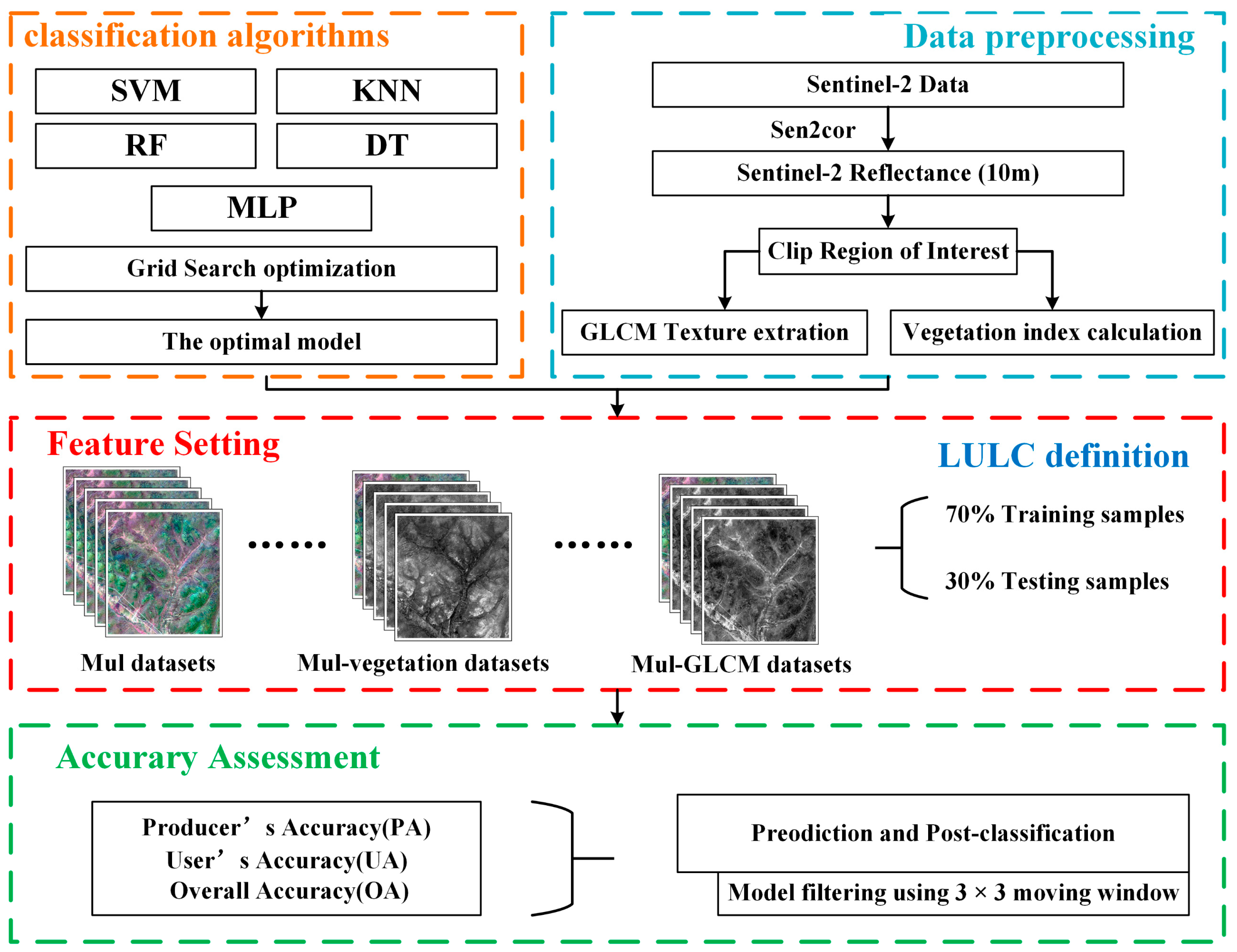
2. Materials and Methods
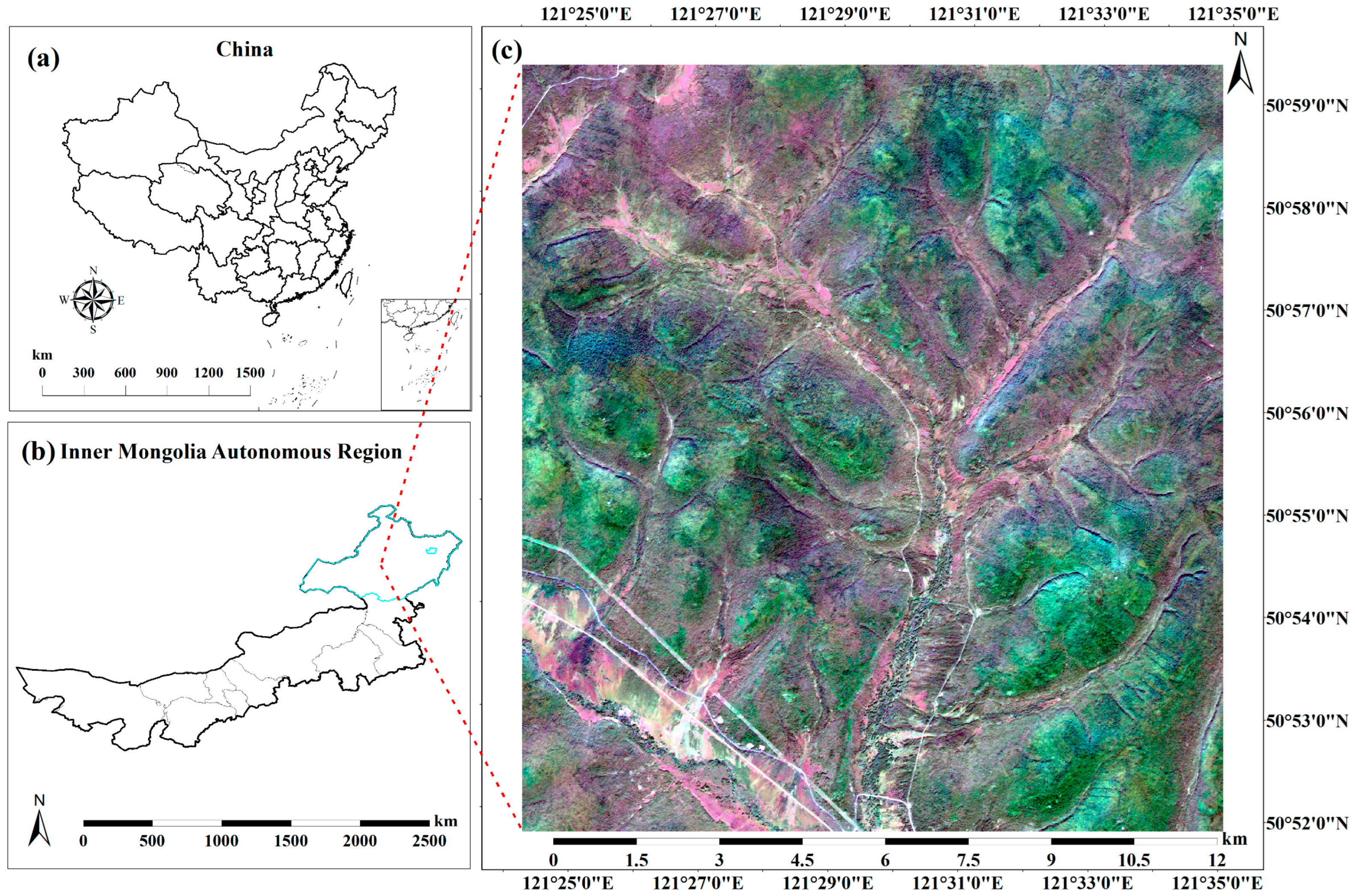
2.1. Study Area
2.2. Data Used
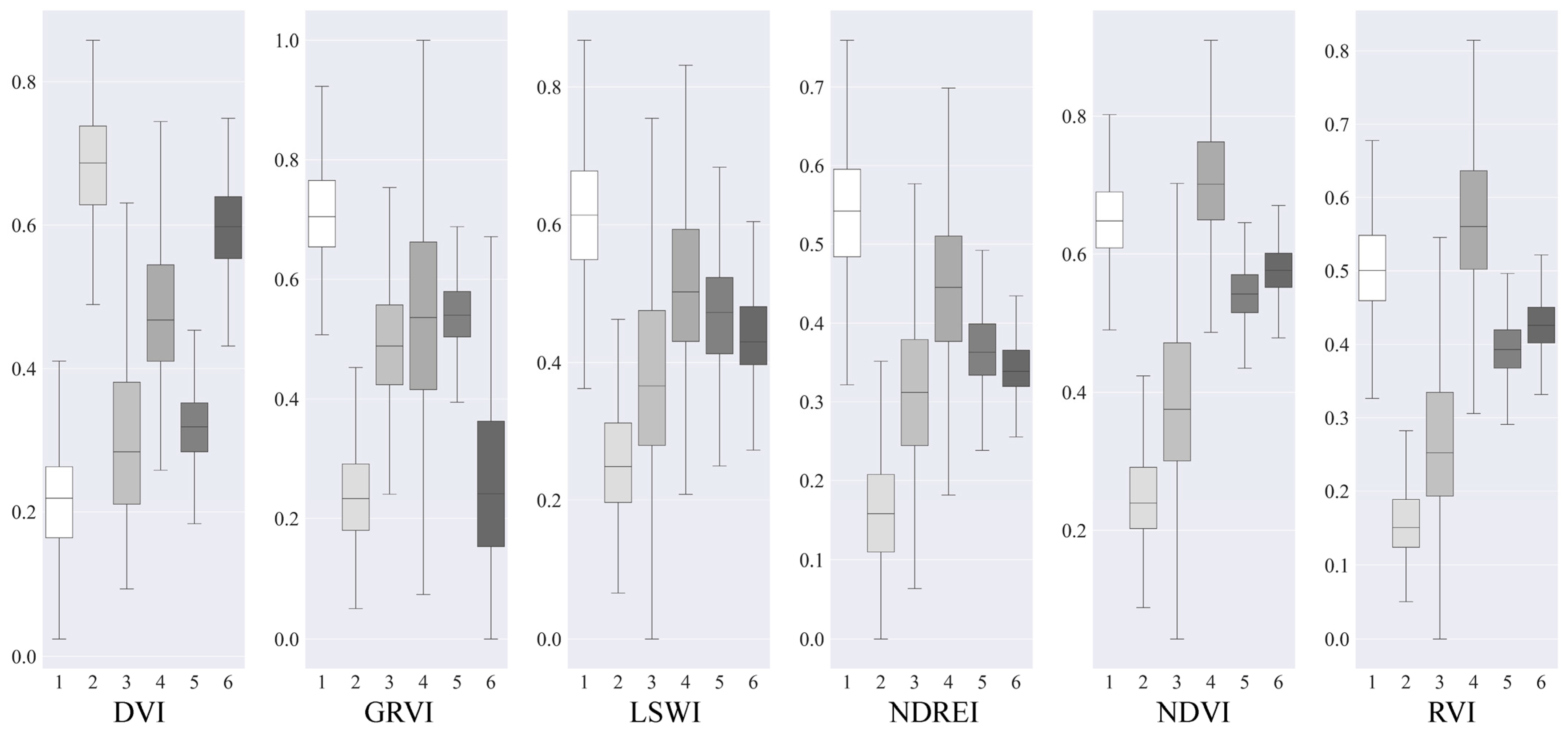
2.3. Feature Setting
2.4. Training Sample Datasets
2.5. Machine Learning Image Classification
2.5.1. Support Vector Machine (SVM)
2.5.2. K-Nearest Neighbor (KNN)
2.5.3. Random Forest (RF)
2.5.4. Decision Trees (DT)
2.5.5. Multi-Layer Perceptron (MLP)
2.6. Accuracy Assessment and Comparisons
3. Results and Analysis
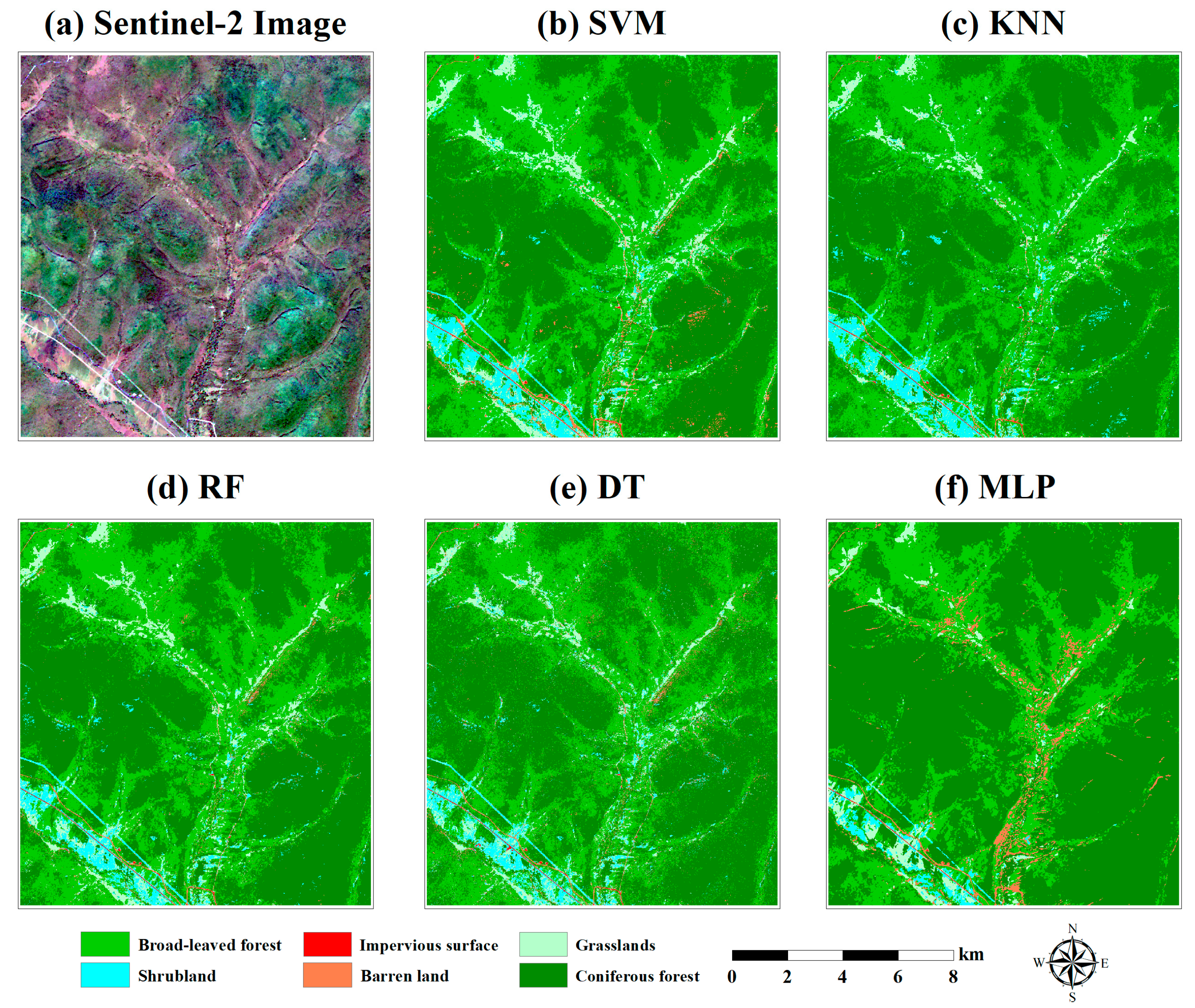
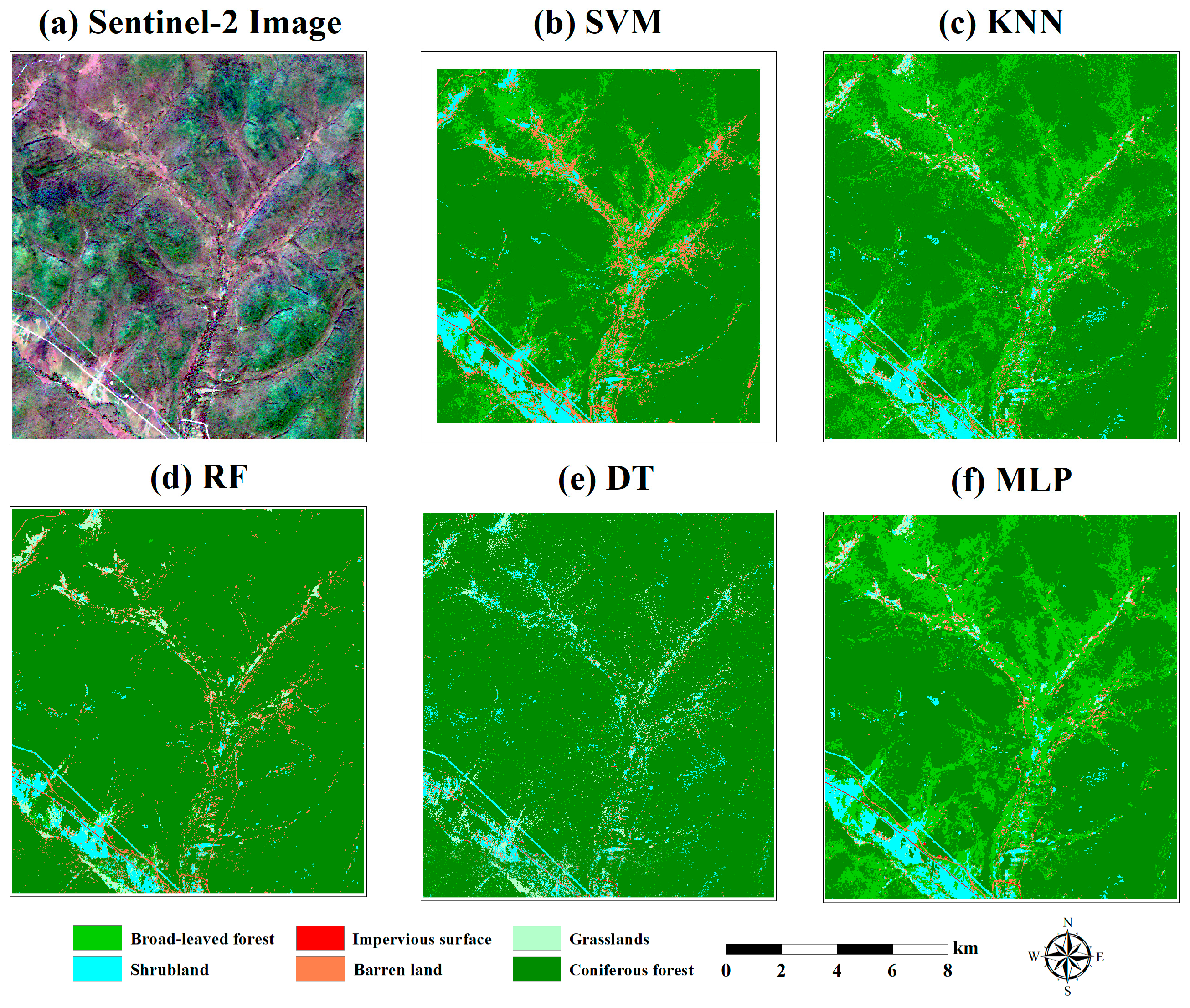
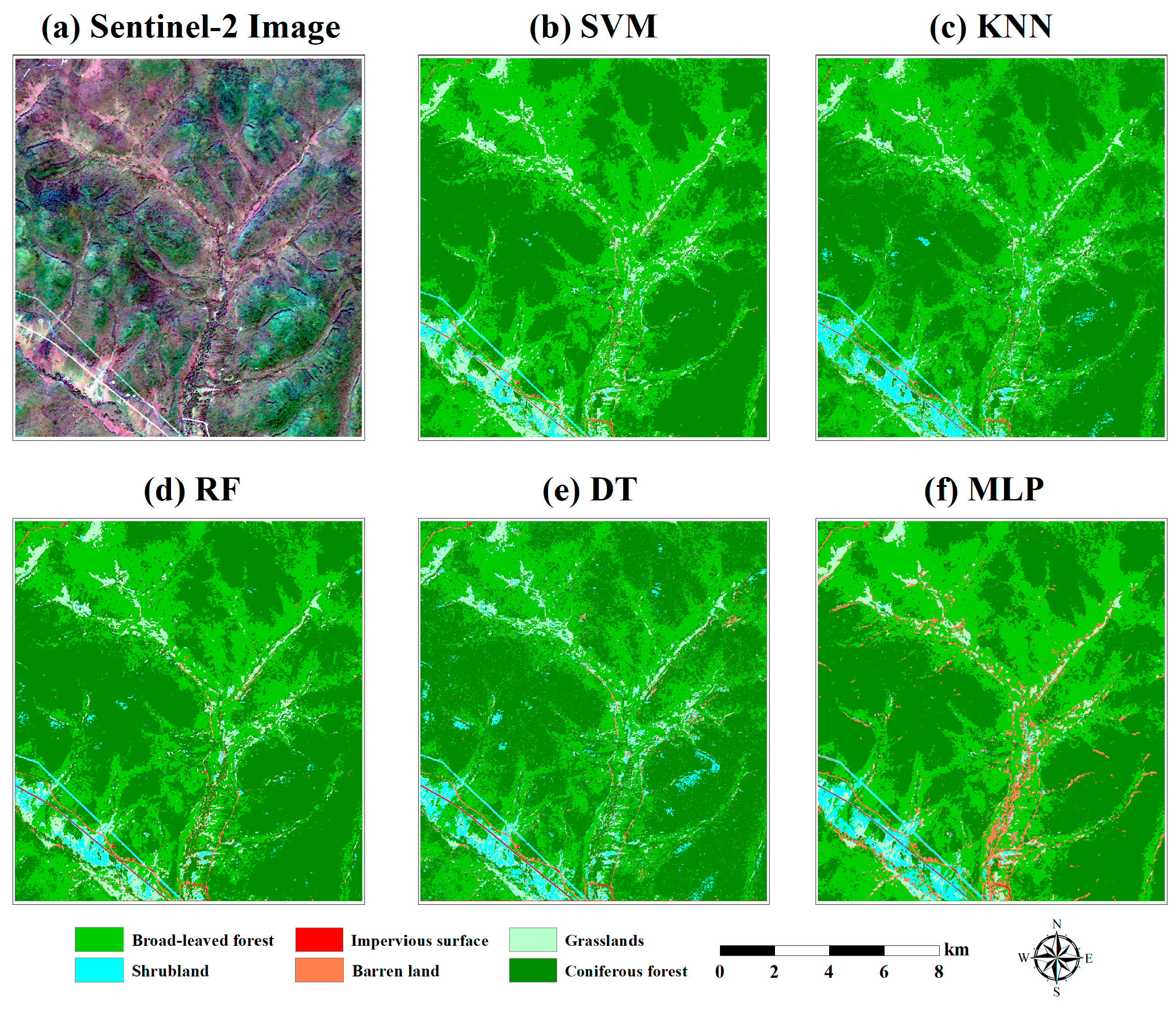
3.1. Forest Land Resource Information Acquisition Results Based on Four Algorithms
- The spatial distribution of forest land resource information based on five classifiers based on Mul:
- The spatial distribution of forest land resource information based on five classifiers based on Mul-vegetation:
- The spatial distribution of forest land resource information based on five classifiers based on Mul-GLCM:
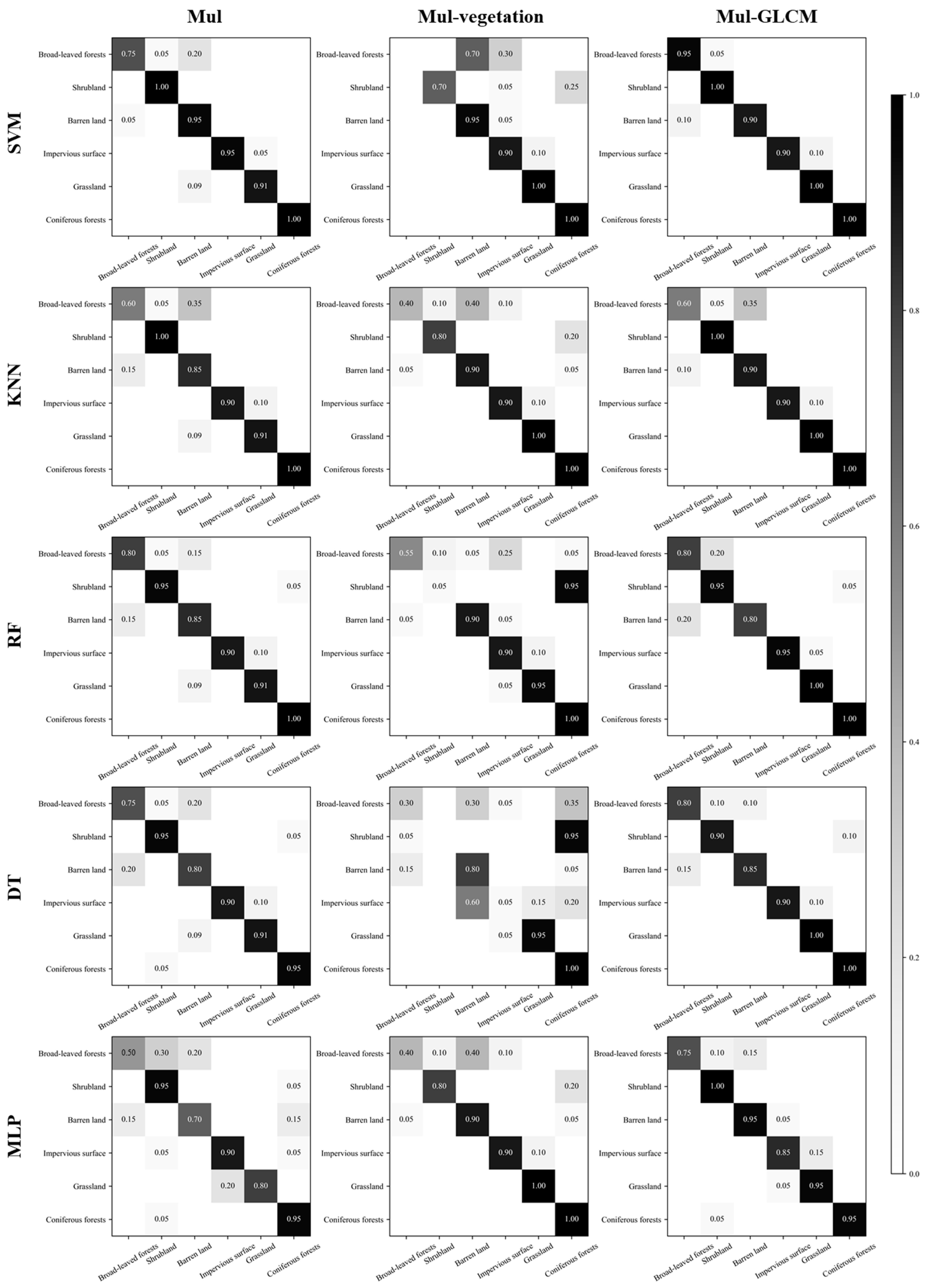
3.2. Forest Land Resource Information Acquisition Confusion Matrix Results Analysis
4. Discussion
5. Conclusions
Author Contributions
Funding
Data Availability Statement
Acknowledgments
Conflicts of Interest
References
- Dotzler, S.; Hill, J.; Buddenbaum, H.; Stoffels, J. The Potential of EnMAP and Sentinel-2 Data for Detecting Drought Stress Phenomena in Deciduous Forest Communities. Remote Sens. 2015, 7, 14227–14258. [Google Scholar] [CrossRef] [Green Version]
- Tian, X.; Yan, M.; van der Tol, C.; Li, Z.; Su, Z.; Chen, E.; Li, X.; Li, L.; Wang, X.; Pan, X.; et al. Modeling Forest Above-Ground Biomass Dynamics Using Multi-Source Data and Incorporated Models: A Case Study over the Qilian Mountains. Agric. For. Meteorol. 2017, 246, 1–14. [Google Scholar] [CrossRef]
- Liu, C.; Tao, R.; Li, W.; Zhang, M.; Sun, M.; Du, Q. Joint Classification of Hyperspectral and Multispectral Images for Mapping Coastal Wetlands. IEEE J. Mag. 2021, 14, 982–996. Available online: https://ieeexplore.ieee.org/abstract/document/9268458 (accessed on 13 November 2022). [CrossRef]
- Szostak, M.; Hawrylo, P.; Piela, D. Using of Sentinel-2 Images for Automation of the Forest Succession Detection. Eur. J. Remote Sens. 2018, 51, 142–149. [Google Scholar] [CrossRef]
- Malinowski, R.; Lewiński, S.; Rybicki, M.; Gromny, E.; Jenerowicz, M.; Krupiński, M.; Nowakowski, A.; Wojtkowski, C.; Krupiński, M.; Krätzschmar, E. Automated Production of a Land Cover/Use Map of Europe Based on Sentinel-2 Imagery. Remote Sens. 2020, 12, 3523. [Google Scholar] [CrossRef]
- Mohammadpour, P.; Viegas, D.X.; Viegas, C. Vegetation Mapping with Random Forest Using Sentinel 2 and GLCM Texture Feature—A Case Study for Lousã Region, Portugal. Remote Sens. 2022, 14, 4585. [Google Scholar] [CrossRef]
- Nelson, M. Evaluating Multitemporal Sentinel-2 Data for Forest Mapping Using Random Forest. Master’s Thesis, Stockholm University, Stockholm, Sweden, 2017. [Google Scholar]
- Hawryło, P.; Bednarz, B.; Wężyk, P.; Szostak, M. Estimating Defoliation of Scots Pine Stands Using Machine Learning Methods and Vegetation Indices of Sentinel-2. Eur. J. Remote Sens. 2018, 51, 194–204. [Google Scholar] [CrossRef] [Green Version]
- Fassnacht, F.E.; Latifi, H.; Stereńczak, K.; Modzelewska, A.; Lefsky, M.; Waser, L.T.; Straub, C.; Ghosh, A. Review of Studies on Tree Species Classification from Remotely Sensed Data. Remote Sens. Environ. 2016, 186, 64–87. [Google Scholar] [CrossRef]
- Wessel, M.; Brandmeier, M.; Tiede, D. Evaluation of Different Machine Learning Algorithms for Scalable Classification of Tree Types and Tree Species Based on Sentinel-2 Data. Remote Sens. 2018, 10, 1419. [Google Scholar] [CrossRef] [Green Version]
- Persson, M.; Lindberg, E.; Reese, H. Tree Species Classification with Multi-Temporal Sentinel-2 Data. Remote Sens. 2018, 10, 1794. [Google Scholar] [CrossRef] [Green Version]
- Guo, Y.; Li, Z.; Chen, E.; Zhang, X.; Zhao, L.; Xu, E.; Hou, Y.; Liu, L. A Deep Fusion UNet for Mapping Forests at Tree Species Levels with Multi-Temporal High Spatial Resolution Satellite Imagery. Remote Sens. 2021, 13, 3613. [Google Scholar] [CrossRef]
- Costa, H.; Benevides, P.; Moreira, F.D.; Moraes, D.; Caetano, M. Spatially Stratified and Multi-Stage Approach for National Land Cover Mapping Based on Sentinel-2 Data and Expert Knowledge. Remote Sens. 2022, 14, 1865. [Google Scholar] [CrossRef]
- Kaplan, G. Broad-Leaved and Coniferous Forest Classification in Google Earth Engine Using Sentinel Imagery. Environ. Sci. Proc. 2020, 3, 64. [Google Scholar] [CrossRef]
- Hernandez, I.; Benevides, P.; Costa, H.; Caetano, M. Exploring Sentinel-2 for Land Cover and Crop Mapping in Portugal. Int. Arch. Photogramm. Remote Sens. Spat. Inf. Sci. 2020, XLIII-B3-2020, 83–89. [Google Scholar] [CrossRef]
- Da Pacheco, A.P.; da Junior, J.A.S.; Ruiz-Armenteros, A.M.; Henriques, R.F.F. Assessment of K-Nearest Neighbor and Random Forest Classifiers for Mapping Forest Fire Areas in Central Portugal Using Landsat-8, Sentinel-2, and Terra Imagery. Remote Sens. 2021, 13, 1345. [Google Scholar] [CrossRef]
- Liu, L.; Guo, Y.; Li, Y.; Zhang, Q.; Li, Z.; Chen, E.; Yang, L.; Mu, X. Comparison of Machine Learning Methods Applied on Multi-Source Medium-Resolution Satellite Images for Chinese Pine (Pinus Tabulaeformis) Extraction on Google Earth Engine. Forests 2022, 13, 677. [Google Scholar] [CrossRef]
- Lu, D.; Weng, Q. A Survey of Image Classification Methods and Techniques for Improving Classification Performance. Int. J. Remote Sens. 2007, 28, 823–870. Available online: https://www.tandfonline.com/doi/full/10.1080/01431160600746456 (accessed on 13 November 2022). [CrossRef]
- Friedl, M.A.; Brodley, C.E. Decision Tree Classification of Land Cover from Remotely Sensed Data. Remote Sens. Environ. 1997, 61, 399–409. [Google Scholar] [CrossRef]
- Waske, B.; Braun, M. Classifier Ensembles for Land Cover Mapping Using Multitemporal SAR Imagery. ISPRS J. Photogramm. Remote Sens. 2009, 64, 450–457. [Google Scholar] [CrossRef]
- Li, C.; Wang, J.; Wang, L.; Hu, L.; Gong, P. Comparison of Classification Algorithms and Training Sample Sizes in Urban Land Classification with Landsat Thematic Mapper Imagery. Remote Sens. 2014, 6, 964–983. [Google Scholar] [CrossRef] [Green Version]
- Hatami, B.; Asadi, F.; Bayani, A.; Zali, M.R.; Kavousi, K. Machine Learning-Based System for Prediction of Ascites Grades in Patients with Liver Cirrhosis Using Laboratory and Clinical Data: Design and Implementation Study. Clin. Chem. Lab. Med. 2022, 60, 1946–1954. [Google Scholar] [CrossRef] [PubMed]
- Garcia-Salgado, B.P.; Ponomaryov, V.I.; Robles-Gonzalez, M.A. Parallel Multilayer Perceptron Neural Network Used for Hyperspectral Image Classification. Proc. SPIE 2016, 9897, 141–153. [Google Scholar]
- Thakur, A.; Mishra, D. Hyper Spectral Image Classification Using Multilayer Perceptron Neural Network & Functional Link ANN. In Proceedings of the 7th International Conference on Cloud Computing, Data Science & Engineering—Confluence, Noida, India, 12–13 January 2017; pp. 639–642. [Google Scholar]
- Kalaiarasi, G.; Maheswari, S. Frost Filtered Scale-Invariant Feature Extraction and Multilayer Perceptron for Hyperspectral Image Classification. arXiv 2020. [Google Scholar] [CrossRef]
- He, X.; Chen, Y. Modifications of the Multi-Layer Perceptron for Hyperspectral Image Classification. Remote Sens. 2021, 13, 3547. [Google Scholar] [CrossRef]
- Delwart, S. ESA Standard Document; European Space Agency: Paris, France, 2015; 64p. [Google Scholar]
- Huang, C.; Davis, L.S.; Townshend, J.R.G. An Assessment of Support Vector Machines for Land Cover Classification. Int. J. Remote Sens. 2002, 23, 725–749. [Google Scholar] [CrossRef]
- Foody, G.M.; Mathur, A. A Relative Evaluation of Multiclass Image Classification by Support Vector Machines. IEEE Trans. Geosci. Remote Sens. 2004, 42, 1335–1343. [Google Scholar] [CrossRef] [Green Version]
- Qian, Y.; Zhou, W.; Yan, J.; Li, W.; Han, L. Comparing Machine Learning Classifiers for Object-Based Land Cover Classification Using Very High Resolution Imagery. Remote Sens. 2015, 7, 153–168. [Google Scholar] [CrossRef]
- Maxwell, A.E.; Warner, T.A.; Fang, F. Implementation of Machine-Learning Classification in Remote Sensing: An Applied Review. Int. J. Remote Sens. 2018, 39, 2784–2817. [Google Scholar] [CrossRef] [Green Version]
- Thanh Noi, P.; Kappas, M. Comparison of Random Forest, k-Nearest Neighbor, and Support Vector Machine Classifiers for Land Cover Classification Using Sentinel-2 Imagery. Sensors 2018, 18, 18. [Google Scholar] [CrossRef] [Green Version]
- Wei, C.; Huang, J.; Mansaray, L.R.; Li, Z.; Liu, W.; Han, J. Estimation and Mapping of Winter Oilseed Rape LAI from High Spatial Resolution Satellite Data Based on a Hybrid Method. Remote Sens. 2017, 9, 488. [Google Scholar] [CrossRef] [Green Version]
- Akbulut, Y.; Sengur, A.; Guo, Y.; Smarandache, F. NS-k-NN: Neutrosophic Set-Based k-Nearest Neighbors Classifier. Symmetry 2017, 9, 179. [Google Scholar] [CrossRef] [Green Version]
- France, S.L.; Douglas Carroll, J.; Xiong, H. Distance Metrics for High Dimensional Nearest Neighborhood Recovery: Compression and Normalization. Inf. Sci. 2012, 184, 92–110. [Google Scholar] [CrossRef]
- Yesilbudak, M.; Sagiroglu, S.; Colak, I. A New Approach to Very Short Term Wind Speed Prediction Using K-Nearest Neighbor Classification. Energy Convers. Manag. 2013, 69, 77–86. [Google Scholar] [CrossRef]
- Belgiu, M.; Drăguţ, L. Random Forest in Remote Sensing: A Review of Applications and Future Directions. ISPRS J. Photogramm. Remote Sens. 2016, 114, 24–31. [Google Scholar] [CrossRef]
- Pal, M. Random Forest Classifier for Remote Sensing Classification. Int. J. Remote Sens. 2005, 26, 217–222. [Google Scholar] [CrossRef]
- Breiman, L. Random Forests. Mach. Learn. 2001, 45, 5–32. [Google Scholar] [CrossRef] [Green Version]
- Huang, J.; Ling, C.X. Using AUC and Accuracy in Evaluating Learning Algorithms. IEEE Trans. Knowl. Data Eng. 2005, 17, 299–310. [Google Scholar] [CrossRef] [Green Version]
- Duro, D.C.; Franklin, S.E.; Dubé, M.G. A Comparison of Pixel-Based and Object-Based Image Analysis with Selected Machine Learning Algorithms for the Classification of Agricultural Landscapes Using SPOT-5 HRG Imagery. Remote Sens. Environ. 2012, 118, 259–272. [Google Scholar] [CrossRef]
- Pal, M.; Mather, P.M. An Assessment of the Effectiveness of Decision Tree Methods for Land Cover Classification. Remote Sens. Environ. 2003, 86, 554–565. [Google Scholar] [CrossRef]
- Han, N.; Du, H.; Zhou, G.; Xu, X.; Ge, H.; Liu, L.; Gao, G.; Sun, S. Exploring the Synergistic Use of Multi-Scale Image Object Metrics for Land-Use/Land-Cover Mapping Using an Object-Based Approach. Int. J. Remote Sens. 2015, 36, 3544–3562. [Google Scholar] [CrossRef]
- Siknun, G.P.; Sitanggang, I.S. Web-Based Classification Application for Forest Fire Data Using the Shiny Framework and the C5.0 Algorithm. Procedia Environ. Sci. 2016, 33, 332–339. [Google Scholar] [CrossRef] [Green Version]
- Tripathi, A.; Tiwari, R.K.; Tiwari, S.P. A Deep Learning Multi-Layer Perceptron and Remote Sensing Approach for Soil Health Based Crop Yield Estimation. Int. J. Appl. Earth Obs. Geoinf. 2022, 113, 102959. [Google Scholar] [CrossRef]
- Rodriguez-Galiano, V.F.; Ghimire, B.; Rogan, J.; Chica-Olmo, M.; Rigol-Sanchez, J.P. An Assessment of the Effectiveness of a Random Forest Classifier for Land-Cover Classification. ISPRS J. Photogramm. Remote Sens. 2012, 67, 93–104. [Google Scholar] [CrossRef]
- Tucker, C.J. Red and Photographic Infrared Linear Combinations for Monitoring Vegetation. Remote Sens. Environ. 1979, 8, 127–150. [Google Scholar] [CrossRef] [Green Version]
- Jurado, J.M.; Ortega, L.; Cubillas, J.J.; Feito, F.R. Multispectral Mapping on 3D Models and Multi-Temporal Monitoring for Individual Characterization of Olive Trees. Remote Sens. 2020, 12, 1106. [Google Scholar] [CrossRef] [Green Version]
- Guan, P.; Zheng, Y.; Lei, G. Analysis of Canopy Phenology in Man-Made Forests Using near-Earth Remote Sensing. Plant Methods 2021, 17, 104. [Google Scholar] [CrossRef]
- Jordan, C.F. Derivation of Leaf-Area Index from Quality of Light on the Forest Floor. Ecology 1969, 50, 663–666. [Google Scholar] [CrossRef]
- Ren, Z.; Rui, G.A.O.; Wang, D. Identification and Classification of Rice Lodging Based on Sentinel-2 Multispectral Image. Water Sav. Irrig. 2022, 7, 44–50. [Google Scholar]
- Yan, Y.-E.; Ouyang, Z.-T.; Guo, H.-Q.; Jin, S.-S.; Zhao, B. Detecting the Spatiotemporal Changes of Tidal Flood in the Estuarine Wetland by Using MODIS Time Series Data. J. Hydrol. 2010, 384, 156–163. [Google Scholar] [CrossRef]
- Chandrasekar, K.; Sesha Sai, M.V.R.; Roy, P.S.; Dwevedi, R.S. Land Surface Water Index (LSWI) Response to Rainfall and NDVI Using the MODIS Vegetation Index Product. Int. J. Remote Sens. 2010, 31, 3987–4005. [Google Scholar] [CrossRef]
- Zhang, X.; Cui, J.; Wang, W.; Lin, C. A Study for Texture Feature Extraction of High-Resolution Satellite Images Based on a Direction Measure and Gray Level Co-Occurrence Matrix Fusion Algorithm. Sensors 2017, 17, 1474. [Google Scholar] [CrossRef] [PubMed] [Green Version]
- Zheng, H.; Du, P.; Chen, J.; Xia, J.; Li, E.; Xu, Z.; Li, X.; Yokoya, N. Performance Evaluation of Downscaling Sentinel-2 Imagery for Land Use and Land Cover Classification by Spectral-Spatial Features. Remote Sens. 2017, 9, 1274. [Google Scholar] [CrossRef] [Green Version]
- Zhao, Y.; Wang, G.; Tang, C.; Luo, C.; Zeng, W.; Zha, Z.-J. A Battle of Network Structures: An Empirical Study of CNN, Transformer, and MLP. arXiv 2021. [Google Scholar] [CrossRef]
- Koukal, T.; Suppan, F.; Schneider, W. The Impact of Relative Radiometric Calibration on the Accuracy of KNN-Predictions of Forest Attributes. Remote Sens. Environ. 2007, 110, 431–437. [Google Scholar] [CrossRef]
- Gjertsen, A.K. Accuracy of Forest Mapping Based on Landsat TM Data and a KNN-Based Method. Remote Sens. Environ. 2007, 110, 420–430. [Google Scholar] [CrossRef]


| Band | Central Wavelength (nm) | Bandwidth (nm) | Spatial Resolution (m) |
|---|---|---|---|
| 2-Blue | 443.9 | 98 | 10 |
| 3-Green | 560.0 | 45 | 10 |
| 4-Red | 664.5 | 38 | 10 |
| 5-Red Edge | 703.9 | 19 | 20 |
| 6-Red Edge | 740.2 | 18 | 20 |
| 7-Red Edge | 782.5 | 28 | 20 |
| 8-NIR | 835.1 | 145 | 10 |
| 8A-Red Edge | 864.8 | 33 | 20 |
| 11-SWIR-1 | 1613.7 | 143 | 20 |
| 12-SWIR-2 | 2202.4 | 242 | 20 |
| Feature Types | Feature Names | Details | Remarks |
|---|---|---|---|
| Vegetation indices | Ratio vegetation index (RVI) | NIR/R | / |
| Difference vegetation index (DVI) | NIR Blue | ||
| Normalized difference vegetation index (NDVI) | (NIR1 R)/(NIR1+ R) | ||
| Green Red Vegetation Index (GRVI) | (Green R)/(Green + R) | ||
| Normalized Difference Red-Edge I Index (NDRE I) | (Red-edge 2 Red-edge 1)/(Red-edge 2 + Red-edge 1) | ||
| Land Surface Water Index (LSWI) | (NIR SWIR-1)/(NIR + SWIR-1) | ||
| Texture features based on the gray-level co-occurrence matrix (GLCM) | Mean (ME) | is the th row of the th column in the th moving window | |
| Variance (VA) | |||
| Entropy (EN) | |||
| Angular second moment (SE) | |||
| Homogeneity (HO) | |||
| Contrast (CON) | |||
| Dissimilarity (DI) | |||
| Correlation (COR) |
| Land Cover | Training Datasets (Objects) | Training Datasets (Pixel) |
|---|---|---|
| Broad-leaved forests | 50 | 691 |
| Shrubland | 50 | 478 |
| Barren land | 50 | 507 |
| Impervious surface | 50 | 504 |
| Grasslands | 50 | 529 |
| Coniferous forests | 50 | 653 |
| SVM | KNN | RF | DT | MLP | ||||||
|---|---|---|---|---|---|---|---|---|---|---|
| Class | PA | UA | PA | UA | PA | UA | PA | UA | PA | UA |
| Broad-leaved forests | 0.750 | 0.938 | 0.600 | 0.800 | 0.800 | 0.842 | 0.750 | 0.790 | 0.500 | 0.769 |
| Shrubland | 1.000 | 0.909 | 1.000 | 0.952 | 0.950 | 0.950 | 1.000 | 0.909 | 0.950 | 0.731 |
| Barren land | 0.950 | 0.826 | 0.850 | 0.708 | 0.850 | 0.850 | 0.800 | 0.800 | 0.700 | 0.778 |
| Impervious surface | 0.950 | 1.000 | 0.900 | 1.000 | 0.900 | 1.000 | 0.900 | 1.000 | 0.900 | 0.818 |
| Grasslands | 1.000 | 0.952 | 1.000 | 0.909 | 1.000 | 0.909 | 1.000 | 0.909 | 0.800 | 1.000 |
| Coniferous forests | 0.950 | 1.000 | 1.000 | 1.000 | 1.000 | 0.952 | 0.950 | 1.000 | 1.000 | 0.800 |
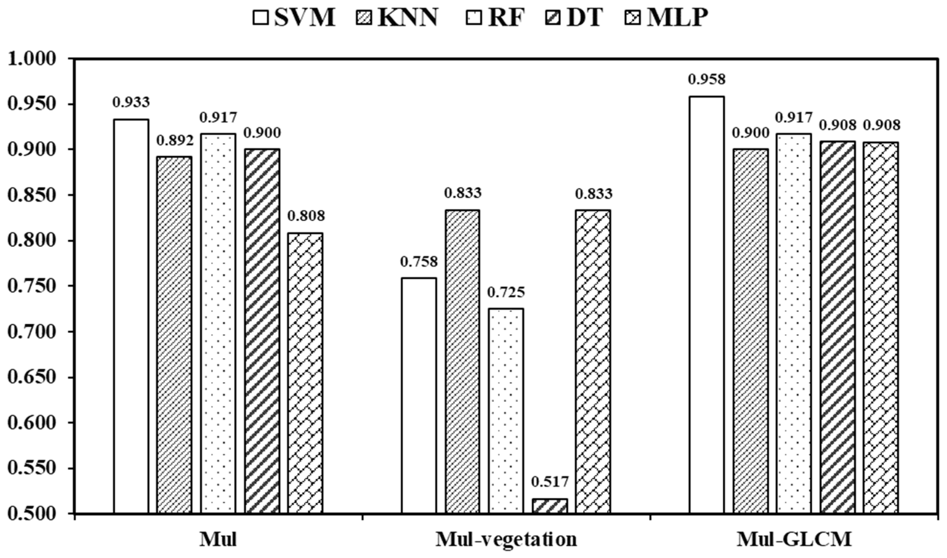
| Overall Accuracy | 0.933 | 0.892 | 0.917 | 0.900 | 0.808 | |||||
| SVM | KNN | RF | DT | MLP | ||||||
|---|---|---|---|---|---|---|---|---|---|---|
| Class | PA | UA | PA | UA | PA | UA | PA | UA | PA | UA |
| Broad-leaved forests | 0.000 | 0.000 | 0.400 | 0.889 | 0.550 | 0.917 | 0.300 | 0.600 | 0.400 | 0.889 |
| Shrubland | 0.700 | 1.000 | 0.800 | 0.889 | 0.050 | 0.333 | 0.000 | 0.000 | 0.800 | 0.889 |
| Barren land | 0.950 | 0.576 | 0.900 | 0.692 | 0.900 | 0.947 | 0.800 | 0.471 | 0.900 | 0.692 |
| Impervious surface | 0.900 | 0.692 | 0.900 | 0.900 | 0.900 | 0.720 | 0.050 | 0.333 | 0.900 | 0.900 |
| Grasslands | 1.000 | 0.909 | 1.000 | 0.909 | 0.950 | 0.905 | 0.950 | 0.864 | 1.000 | 0.909 |
| Coniferous forests | 1.000 | 0.800 | 1.000 | 0.800 | 1.000 | 0.500 | 1.000 | 0.392 | 1.000 | 0.800 |
| Overall Accuracy | 0.758 | 0.833 | 0.725 | 0.517 | 0.833 | |||||
| SVM | KNN | RF | DT | MLP | ||||||
|---|---|---|---|---|---|---|---|---|---|---|
| Class | PA | UA | PA | UA | PA | UA | PA | UA | PA | UA |
| Broad-leaved forests | 0.950 | 0.905 | 0.600 | 0.857 | 0.800 | 0.800 | 0.800 | 0.842 | 0.750 | 1.000 |
| Shrubland | 1.000 | 0.952 | 1.000 | 0.952 | 0.950 | 0.826 | 0.900 | 0.900 | 1.000 | 0.870 |
| Barren land | 0.900 | 1.000 | 0.900 | 0.720 | 0.800 | 1.000 | 0.850 | 0.895 | 0.950 | 0.864 |
| Impervious surface | 0.900 | 1.000 | 0.900 | 1.000 | 0.950 | 1.000 | 0.900 | 1.000 | 0.850 | 0.895 |
| Grasslands | 1.000 | 0.909 | 1.000 | 0.909 | 1.000 | 0.952 | 1.000 | 0.909 | 0.950 | 0.864 |
| Coniferous forests | 1.000 | 1.000 | 1.000 | 1.000 | 1.000 | 0.952 | 1.000 | 0.909 | 0.950 | 1.000 |
| Overall Accuracy | 0.958 | 0.900 | 0.917 | 0.908 | 0.908 | |||||
Disclaimer/Publisher’s Note: The statements, opinions and data contained in all publications are solely those of the individual author(s) and contributor(s) and not of MDPI and/or the editor(s). MDPI and/or the editor(s) disclaim responsibility for any injury to people or property resulting from any ideas, methods, instructions or products referred to in the content. |
© 2023 by the authors. Licensee MDPI, Basel, Switzerland. This article is an open access article distributed under the terms and conditions of the Creative Commons Attribution (CC BY) license (https://creativecommons.org/licenses/by/4.0/).
Share and Cite
Zhang, C.; Liu, Y.; Tie, N. Forest Land Resource Information Acquisition with Sentinel-2 Image Utilizing Support Vector Machine, K-Nearest Neighbor, Random Forest, Decision Trees and Multi-Layer Perceptron. Forests 2023, 14, 254. https://doi.org/10.3390/f14020254
Zhang C, Liu Y, Tie N. Forest Land Resource Information Acquisition with Sentinel-2 Image Utilizing Support Vector Machine, K-Nearest Neighbor, Random Forest, Decision Trees and Multi-Layer Perceptron. Forests. 2023; 14(2):254. https://doi.org/10.3390/f14020254
Chicago/Turabian StyleZhang, Chen, Yang Liu, and Niu Tie. 2023. "Forest Land Resource Information Acquisition with Sentinel-2 Image Utilizing Support Vector Machine, K-Nearest Neighbor, Random Forest, Decision Trees and Multi-Layer Perceptron" Forests 14, no. 2: 254. https://doi.org/10.3390/f14020254