Estimation of Extreme Daily Rainfall Probabilities: A Case Study in Kyushu Region, Japan

Abstract

Extreme rainfall causes floods and landslides, and so damages humans and socioeconomics; for instance, floods and landslides have been triggered by repeated torrential precipitation and have caused severe damage in the Kyushu region, Japan. Therefore, evaluating extreme rainfall in Kyushu is necessary to provide basic information for measures of rainfall-induced disasters. In this study, we estimated the probability of daily rainfall in Kyushu. The annual maximum values for daily rainfall at 23 long-record stations were normalized using return values at each station, corresponding to 2 and 10 years, and were combined by the station-year method. Additionally, the return period (RP) was calculated by fitting them to the generalized extreme value distribution. Based on the relationship between the normalized values of annual maximum daily rainfall and the RP, we obtained a regression equation to accurately estimate the RP up to 300 years by using data at given stations, considering outliers. In addition, we verified this equation using data from short-record stations where extreme rainfall events triggering floods and landslides were observed, and thereby elucidated that our method was consistent with previous techniques. Thus, this study develops strategies of measures for floods and landslides.

1. Introduction

Extreme rainfall is an inducing factor for floods and landslides, which cause severe damage to humans and socioeconomics [1,2,3]. Hagon et al. [1] investigated six types of climate- and weather-related disasters (flood, storm, hydrometeorological landslide, wildfire, extreme temperature, and drought) worldwide between 1960 and 2020 and showed that floods affect more people globally than any other disaster. Ushiyama and Yokomaku [3] evaluated six types of disasters induced by heavy rainfall (storm surge, strong wind, flood, landslide, water accident in rivers excluding flood, and others) in Japan between 2004 and 2011. They showed that the number of deaths due to landslides was the highest and due to floods was the second highest [3]. In addition, increases in precipitation influenced by climate change are likely to increase floods and landslides [4,5,6].

Japan is within the East Asian monsoon region where torrential rainfall is frequent during the summer monsoon [7], and so floods and rainfall-induced landslides occur commonly and often cause damage [8]. In the Kyushu region, floods and landslides have occurred repeatedly [9,10,11,12] and may have been affected by climate change in recent years [13,14]; for example, an extreme rainfall event in the northern part of Kyushu in July 2017 induced severe damage from landslides, driftwood, and floods [12]. Thus, to mitigate the damage from floods and landslides, it is necessary to evaluate rainfall characteristics that may cause these disasters.

Rainfall frequency analysis statistically evaluates the magnitude of rainfall characteristics and provides basic information for the planning, design, and management of hydraulic structures (e.g., check dam and culvert) [15,16,17,18]. Similarly, rainfall frequency analysis is required in case studies of catastrophic disasters [15,19]. Hence, many researchers proposed theories for evaluating extreme rainfall (e.g., [20,21,22,23]). However, the rainfall record in the individual site is generally less than the return period (RP) required to design hydraulic structures [19]. Moreover, the record at one station may not include extreme rainfall because extreme rainfall is low frequency and has spatial heterogeneity [24]. Consequently, the results of rainfall frequency analysis may include uncertainty.

Regional frequency analysis (e.g., [25,26,27,28]) addresses these problems by using rainfall data observed at all stations in the region. The station-year method [15,16] combines the rescaled data from all stations into a single sample and fits a distribution by treating the combined sample as a single random sample [27]. Hosking and Wallis [27] mentioned that this method was rarely used because it is not appropriate to treat the rescaled data as a single random sample in many cases. Nevertheless, the station-year method has been used even in recent years (e.g., [29,30,31]) due to its simplicity.

In Japan, Suzuki and Kikuchihara [24] applied the station-year method to the annual maximum daily rainfall data from 137 stations and estimated the probability of extreme daily rainfall. They showed that daily rainfall for RP up to 1000 years was estimated successfully in the region using the return values of 2 and 10 years estimated by the plotting position formula (Hazen’s formula) at a given station [24]. However, there was no comparison between the RPs estimated by their technique and by other processes at individual stations where extreme rainfall events occurred, that is, the usefulness and validation of their method were not sufficiently evaluated. In addition, rainfall data were not examined to the same standard because the periods for calculating the return values were different for each station.

The purpose of this study is to estimate regional daily rainfall in Kyushu by improving the previous method [24]. Additionally, we also examine the usefulness and limitations of our method in terms of development measures against floods and landslides. In this paper, we first describe the procedures for normalizing and combining daily rainfall at 23 stations in Kyushu, respectively (Section 2). Next, we examine the relationship between the RP and the normalized daily rainfall and propose an empirical dependence for estimating daily rainfall (Section 3.4). Then, we validate our method using daily rainfall data from short-record stations, including extreme events (Section 3.5). Lastly, we discuss the usefulness and limitations of our method (Section 3.6).

2. Materials and Methods

2.1. Analysis Procedure

The method of this study is divided into four steps. First, the data for the annual maximum daily rainfall in the Kyushu region are collected. Next, the spatial correlation of rainfall data between the two stations is investigated. Following this, the annual maximum daily rainfall is normalized using quantiles, corresponding to the non-exceedance probability of 50% and 90% of the generalized extreme value (GEV) distribution. The second and third steps are performed to apply the station-year method. Then, the normalized rainfall data are combined and converted to the RP.

2.2. Data Collection

The annual maximum value for daily rainfall at 23 meteorological observatories operated by the Japan Meteorological Agency (JMA) in Kyushu until 2020 was used to estimate the RP of daily rainfall because long-term records are available (Figure 1 and

Table 1. Specifications of meteorological observatories in Kyushu.

Name	Location			Observation Period (Start Year)
	X	Y	Z (m)
Fukuoka	130°22.5′ E	33°34.9′ N	2.5	131 (1890~)
Izuka	130°41.6′ E	33°39.1′ N	37.5	86 (1935~)
Oita	131°37.1′ E	33°19.3′ N	4.6	134 (1887~)
Hita	130°55.7′ E	33°19.3′ N	82.9	79 (1942~)
Saga	130°18.3′ E	33°15.9′ N	5.5	131 (1890~)
Hirado	129°33.0′ E	33°09.5′ N	57.8	81 (1940~)
Sasebo	129°43.6′ E	33°09.5′ N	3.9	75 (1946~)
Nagasaki	129°52.0′ E	32°44.0′ N	26.9	143 (1978~)
Unzen	130°15.7′ E	32°44.2′ N	677.5	97 (1924~)
Fukue	128°49.6′ E	32°41.6′ N	25.1	59 (1962~)
Induhara	129°17.5′ E	34°11.8′ N	3.7	135 (1886~)
Kamamato	130°42.4′ E	32°11.8′ N	37.7	131 (1890~)
Ushibuka	130°01.6′ E	32°11.8′ N	3.0	72 (1949~)
Hitoyoshi	130°45.3′ E	32°13.0′ N	145.8	78 (1943~)
Nobeoka	131°39.4′ E	32°34.9′ N	19.2	60 (1961~)
Aburatsu	131°22.4′ E	31°34.7′ N	2.9	72 (1949~)
Miyakonojo	131°04.9′ E	31°43.8′ N	153.8	79 (1942~)
Miyazaki	131°24.8′ E	31°56.3′ N	9.2	135 (1886~)
Akune	130°12.0′ E	32°01.6′ N	40.1	82 (1939~)
Kagoshima	130°32.8′ E	31°33.3′ N	3.9	138 (1883~)
Makurazaki	130°17.5′ E	31°16.3′ N	29.5	98 (1923~)
Yakushima	130°39.5′ E	30°23.1′ N	37.3	84 (1937~)
Tanegashima	130°58.9′ E	30°43.2′ N	24.9	73 (1948~)

). The longest record is 143 years at Nagasaki, the shortest is 59 years at Fukue, and the average for the 23 sites is 98 years. The highest elevation at the rainfall station is 677.5 m at Unzen, the lowest is 2.5 m at Fukuoka, and the average is 20.6 m. The distance between the stations is 25.0 km at the shortest and 441.8 km at the longest.

In addition, the annual maximum value for daily rainfall until 2020 from the Automated Meteorological Data Acquisition System (AMeDAS) Izumi, Morotsuka, Aso-Otohime, and Asakura operated by the JMA was used to validate our method (Figure 1). These stations were selected because they have short-period records (approximately 40 years) and observed extreme rainfall events that triggered floods and landslides (

Table 2. Specifications of AMeDAS.

AMeDAS	Location			Occurrence of Disasters (Year)	References
	X	Y	Z (m)
Asakura	130°41.7′ E	33°24.4′ N	38.0	2017	Takahashi et al. (2021) [12]
Aso-Otohime	131°02.4′ E	32°56.8′ N	487.0	1990 2012	Ishikawa and Shida (1990) [32] Yang et al. (2015) [34]
Izumi	130°21.1′ E	32°05.6′ N	11.0	1997	Sassa (1998) [33]
Morotsuka	131°20.1′ E	32°31.0′ N	150.0	2005	Chigira (2005) [9]

) [12,32,33,34]. Specifically, a rainfall event that triggered a deep-seated landslide and debris flow was observed at AMeDAS Izumi in July 1997. At AMeDAS Morotsuka, a rainfall event that triggered deep-seated landslides was observed in September 2005. At AMeDAS Aso-Otohime, rainfall events that triggered floods and debris flow were observed in July 1990 and July 2012, respectively. At AMeDAS Asakura, an extreme rainfall event that triggered shallow landslides and debris flow including driftwood was observed in July 2017.

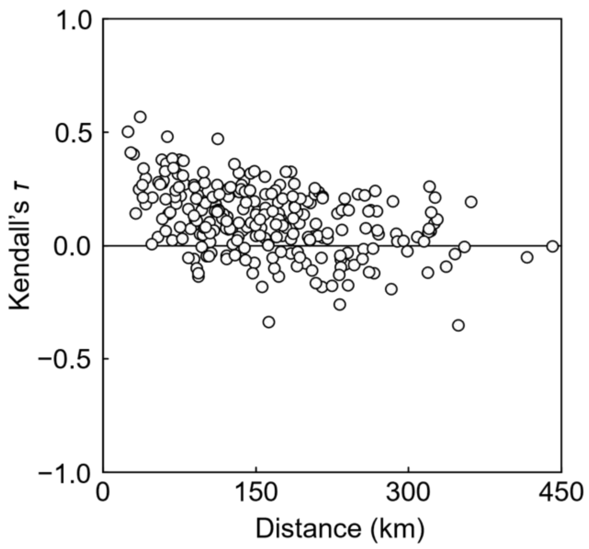
2.3. Investigation of Spatial Correlation of Annual Maximum Value for Daily Rainfall

The Kendall rank correlation coefficient (Kendall’s τ) [35] of the annual maximum daily rainfall between two stations was investigated because the station-year method assumes the spatial independence of stations [17]. In previous studies [17,28,30,36], spatial independence was investigated using Pearson’s correlation coefficient, but Kendall’s τ was used in this study since the annual maximum daily rainfall between two stations was not assumed to be Gaussian distribution.

Kendall’s τ is a non-parametric method for testing the dependence between two variables based on an ordinal association between two measured quantities. Kendall’s τ is given as:

$$\tau =\frac{{{\displaystyle \sum }}_{i<j}sign\left(x_i-x_j\right)sign\left(y_i-y_j\right)}{n\left(n-1\right)∕2}$$

(1)

where sign (⋅) is the sign function. To conduct this investigation, common period data from all stations between 1981 and 2010 were used.

2.4. Normalization of Daily Rainfall Data

Quantiles corresponding to the non-exceedance probability of 50% and 90% were used to normalize the daily rainfall data; in other words, the values corresponding to the RP of 2 and 10 years (2- and 10-year values). These indices were less variable since they were calculated by interpolation at each station and were considered suitable for normalization. Suzuki and Kikuchihara [24] also used 2- and 10-year values to normalize the daily rainfall data. The data for the annual maximum daily rainfall were normalized following Suzuki and Kikuchihara [24]:

$$y_T=\frac{x_j-x_2}{x_{10}-x_2}$$

(2)

where y_T is normalized daily rainfall and x_j is the annual maximum daily rainfall. x₂ and x₁₀ are the 2- and 10-year values, respectively.

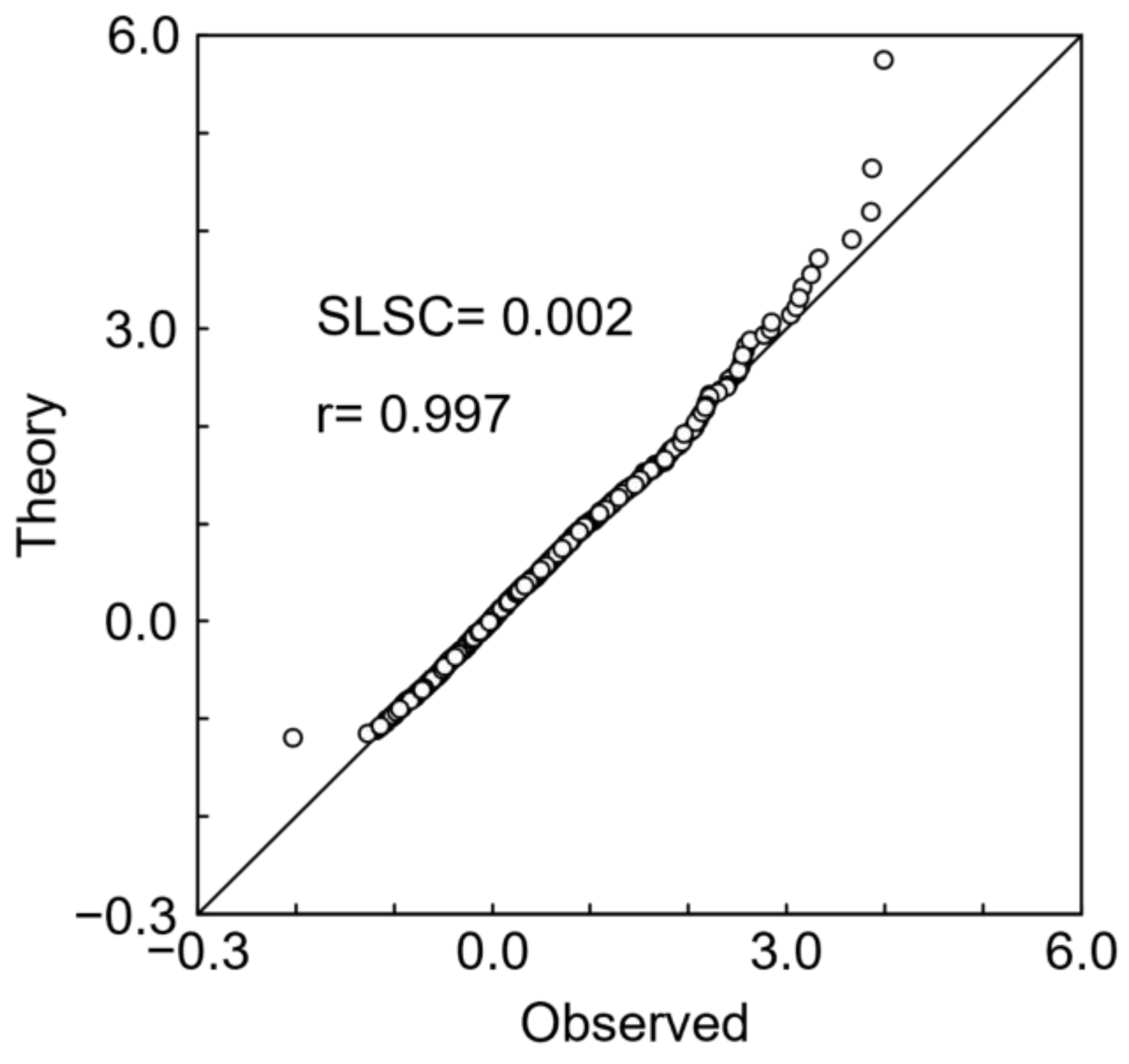
2.5. Extreme Value Analysis

The 2- and 10-year values were calculated using parameters in the GEV distribution [22], estimated by the L-moment method [21]. The data for the annual maximum daily rainfall between 1981 and 2010 were used due to the need to unify the period for calculating the GEV parameters. The GEV cumulative distribution function and the quantile of the GEV corresponding to the non-exceedance probability are given as, respectively:

$$F\left(x\right)=exp\left\{-{\left(1-k\frac{x-c}{a}\right)}^{\frac{1}{k}}\right\} \mathrm{for} k\ne 0$$

(3)

$$x_p=c+\frac{a}{k}[1-{\left\{-\ln \left(p\right)\right\}}^k]$$

(4)

where k is the shape parameter, c is the scale parameter, a is the location parameter, and p is the non-exceedance probability. The parameters of the GEV are given as:

$$\{\begin{array}{l}k=7.8590d+2.9554d^2\\ a={\displaystyle \frac{k{\lambda }_2}{\left(1-2^{-k}\right)\mathsf{\Gamma }\left(1+k\right)}}\\ c={\lambda }_1-\frac{a}{k}\left\{1-\mathsf{\Gamma }\left(1+k\right)\right\}\end{array}$$

(5)

$$d=\frac{2{\lambda }_2}{{\lambda }_3+3{\lambda }_2}-\frac{\ln \left(2\right)}{\ln \left(3\right)}$$

(6)

where λ_1–3 are sample L-moments and Γ the gamma function. λ_1–3 are given as:

$$\{\begin{array}{l}{\lambda }_1={\beta }_0={\displaystyle \frac{1}{N}}{\displaystyle {\displaystyle \sum }_{j=1}^N}{x}_{\left(j\right)}\\ {\lambda }_2={\beta }_1={\displaystyle \frac{1}{N\left(N-1\right)}}{\displaystyle {\displaystyle \sum }_{j=1}^N}\left(j-1\right)x_{\left(j\right)}\\ {\lambda }_3={\beta }_2={\displaystyle \frac{1}{N\left(N-1\right)\left(N-2\right)}}{\displaystyle {\displaystyle \sum }_{j=1}^N}\left(j-1\right)\left(j-2\right)x_{\left(j\right)}\end{array}$$

(7)

where x_(j) is the j-th value from the smallest when the sample is arranged in increasing order.

The standard least-squares criterion (SLSC) [37,38] was used to evaluate the goodness of fit between the observed rainfall and the probability distribution. The SLSC compares the goodness of fit across distributions, and their smaller values imply better fits [37]. In this study, we judged a good fit when the SLSC value was below 0.04 in accordance with the JMA [39]. The SLSC value is given as:

$$SLSC=\frac{\sqrt{{\displaystyle \frac{1}{N}}{{\displaystyle \sum }}_{j=1}^N{\left\{s\left(x_{\left(j\right)}\right)-s^{*}\left(p_{\left(j\right)}\right)\right\}}^2}}{\left|s_{0.99}-s_{0.01}\right|}$$

(8)

$$s(x_{\left(j\right)})=-\ln \left[\left\{{\left(1-k\frac{x_{\left(j\right)}-c}{a}\right)}^{\frac{1}{k}}\right\}\right]$$

(9)

$$s^{*}\left(p_{\left(j\right)}\right)=-\ln \left[-\ln \left\{p_{\left(j\right)}\right\}\right]$$

(10)

where s(x_(j)) is the standardized variate by GEV parameters and s*(p_(j)) is the standardized variate corresponding to the non-exceedance probability calculated by the plotting position formula [40]. s_0.99 and s_0.01 are the standardized variates corresponding to the non-exceedance probability of 1% and 99%, respectively. The plotting position formula is given as:

$$p_{\left(j\right)}=F\left(x_{\left(j\right)}\right)=\frac{j-\alpha }{N+1-2\alpha }$$

(11)

where α is a constant; we used Cunnane’s formula (α = 0.4) [41] to give p_i following the JMA [39].

3. Results and Discussion

3.1. Spatial Correlation of Annual Maximum Value Daily Rainfall between 1981 and 2010

Figure 2 shows Kendall’s τ of the annual maximum daily rainfall between two stations plotted against distance. As shown in Figure 2, Kendall’s τ of the annual maximum daily rainfall between two stations tended to decrease as the distance between the two stations increased. In general, the correlation of rainfall decreases [17,28,30,36]; for example, Kuzuha et al. [34] examined the spatial correlation structure of precipitation using rainfall data at AMeDAS in Japan and showed that Pearson’s correlation coefficient of daily rainfall decreased exponentially as the distance between the two stations increased. Hence, our result agreed with previous studies.

Furthermore, Kendall’s τ of the annual maximum daily rainfall between two stations was 0.57 at its maximum and was generally small (Figure 2). Overeem et al. [17] examined the spatial dependence to apply the station-year method by using Pearson’s correlation coefficient of daily rainfall between the two stations. They assumed the spatial dependence even if the Pearson’s correlation coefficient was around 0.60 [17]. Although the Kendall’s τ and Pearson’s correlation coefficient were not simply comparable, we believed that the data for the annual maximum daily rainfall at 23 stations were spatially independent considering a previous study [17].

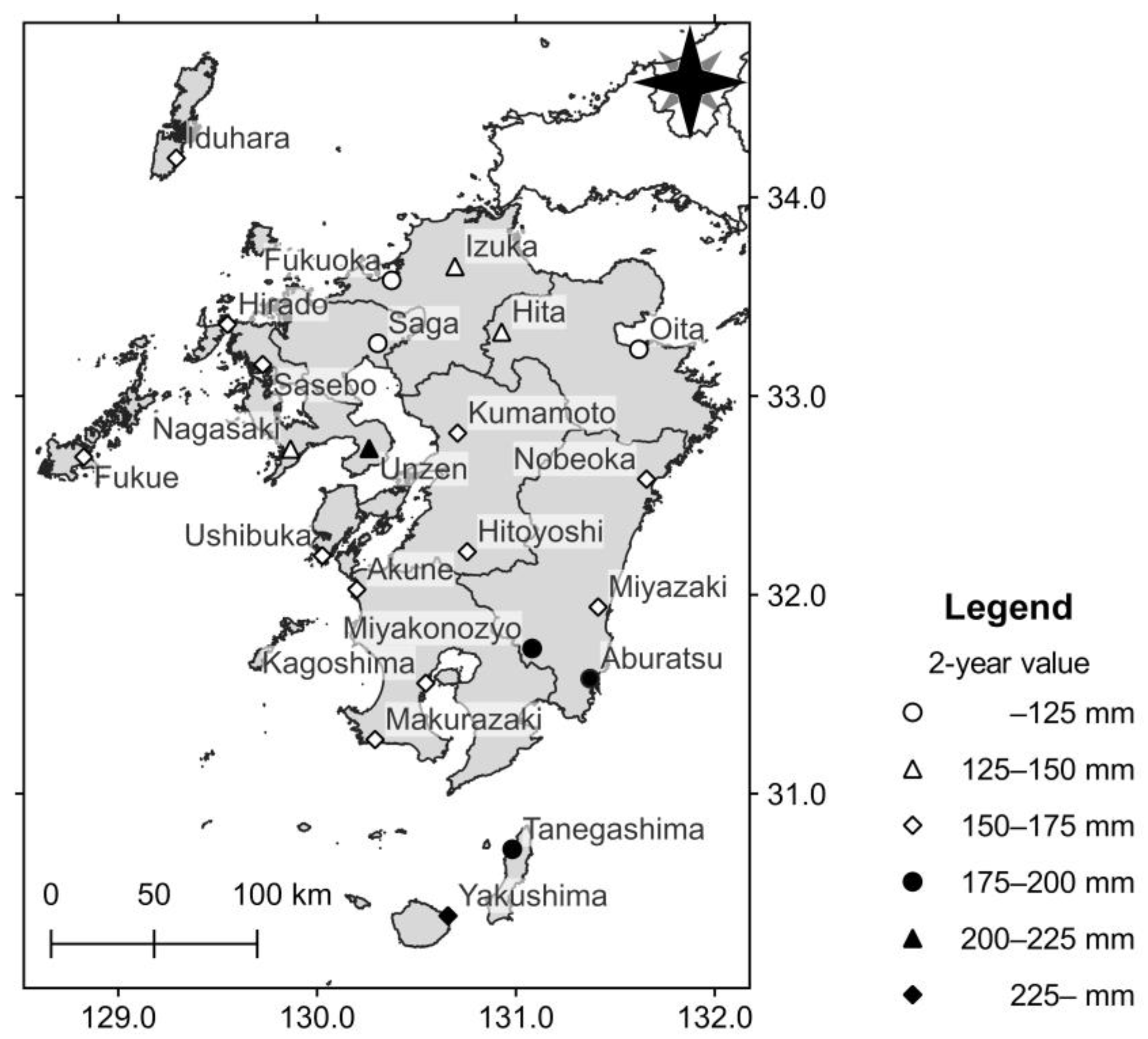
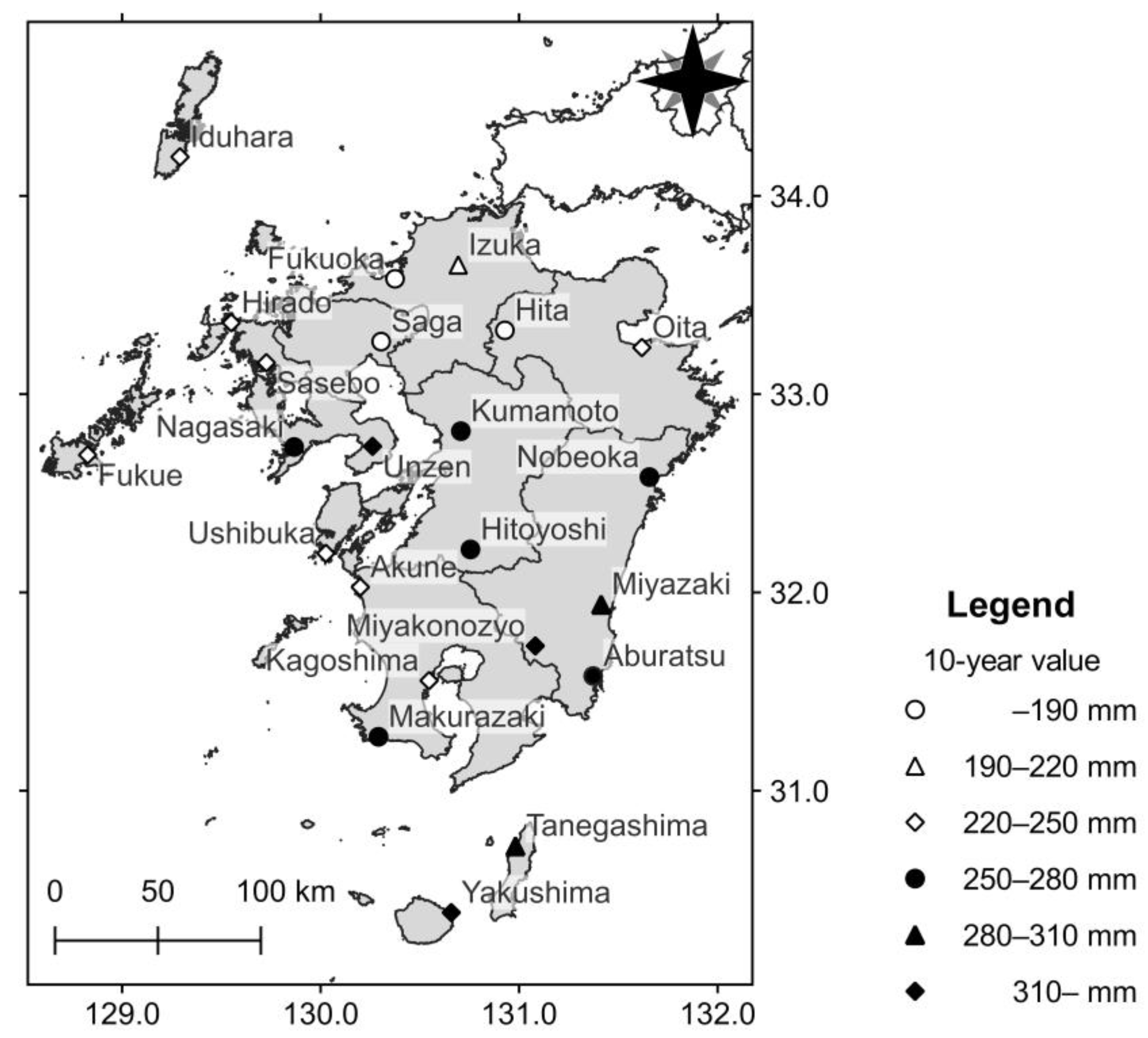
3.2. Spatial Distribution of 2- and 10-Year Values

Table 3. The 2- and 10-year values at long-term record stations.

Name	2-Year Value	10-Year Value	SLSC
Fukuoka	121.6	182.7	0.019
Izuka	131.1	213.6	0.026
Oita	124.4	240.2	0.031
Hita	126.1	178.6	0.018
Saga	124.4	186.8	0.022
Hirado	159.4	239.0	0.006
Sasebo	150.2	242.7	0.024
Nagasaki	130.4	250.6	0.033
Unzen	207.3	330.8	0.021
Fukue	152.7	273.7	0.028
Induhara	160.2	243.9	0.024
Kamamato	166.2	276.6	0.023
Ushibuka	146.2	246.1	0.024
Hitoyoshi	161.2	254.0	0.027
Nobeoka	172.2	265.3	0.021
Aburatsu	176.1	271.6	0.022
Miyakonojo	180.7	310.4	0.028
Miyazaki	166.8	293.1	0.028
Akune	144.2	256.1	0.021
Kagoshima	158.8	234.4	0.022
Makurazaki	155.9	253.6	0.030
Yakushima	241.0	341.8	0.022
Tanegashima	176.5	284.5	0.019

shows the 2- and 10-year values and the SLSC for each station. As shown in Table 3, the SLSC values at all stations were below the JMA criterion (0.04) [39]; therefore, the observed rainfall and GEV distribution were a good fit.

Figure 3 and Figure 4 show the spatial distribution of the 2- and 10-year values, respectively. As shown in Figure 3 and Figure 4, the 2- and 10-year values tended to be lower in the northern plains and were larger in the south, especially in the east of the Kyushu Mountains. At the Fukuoka Regional Headquarters, the JMA [42] investigated the relationship between the spatial distribution of annual precipitation and the topographical conditions in northern Kyushu Island. They showed that the annual precipitation on the plain in the north was smaller than in the mountainous areas, the eastern hillsides near the Kyushu Mountains had more precipitation due to the influence of typhoons, and the annual precipitation at 32–33° N was higher than that of around 34° N because this area was affected by typhoons and Baiu precipitation [42]. Moreover, the JMA [39] examined the spatial distribution of probable rainfall for 30, 50, 100, and 200 years using the annual maximum daily rainfall between 1901 and 2006 at 51 sites nationwide and showed that the probable rainfall in the Kyushu region (Fukuoka, Oita, Nagasaki, Kumamoto, Miyazaki, and Kagoshima) tended to be smaller in the north, but larger in the south. Thus, the 2- and 10-year values represented the regional rainfall characteristics and were good indexes for normalization.

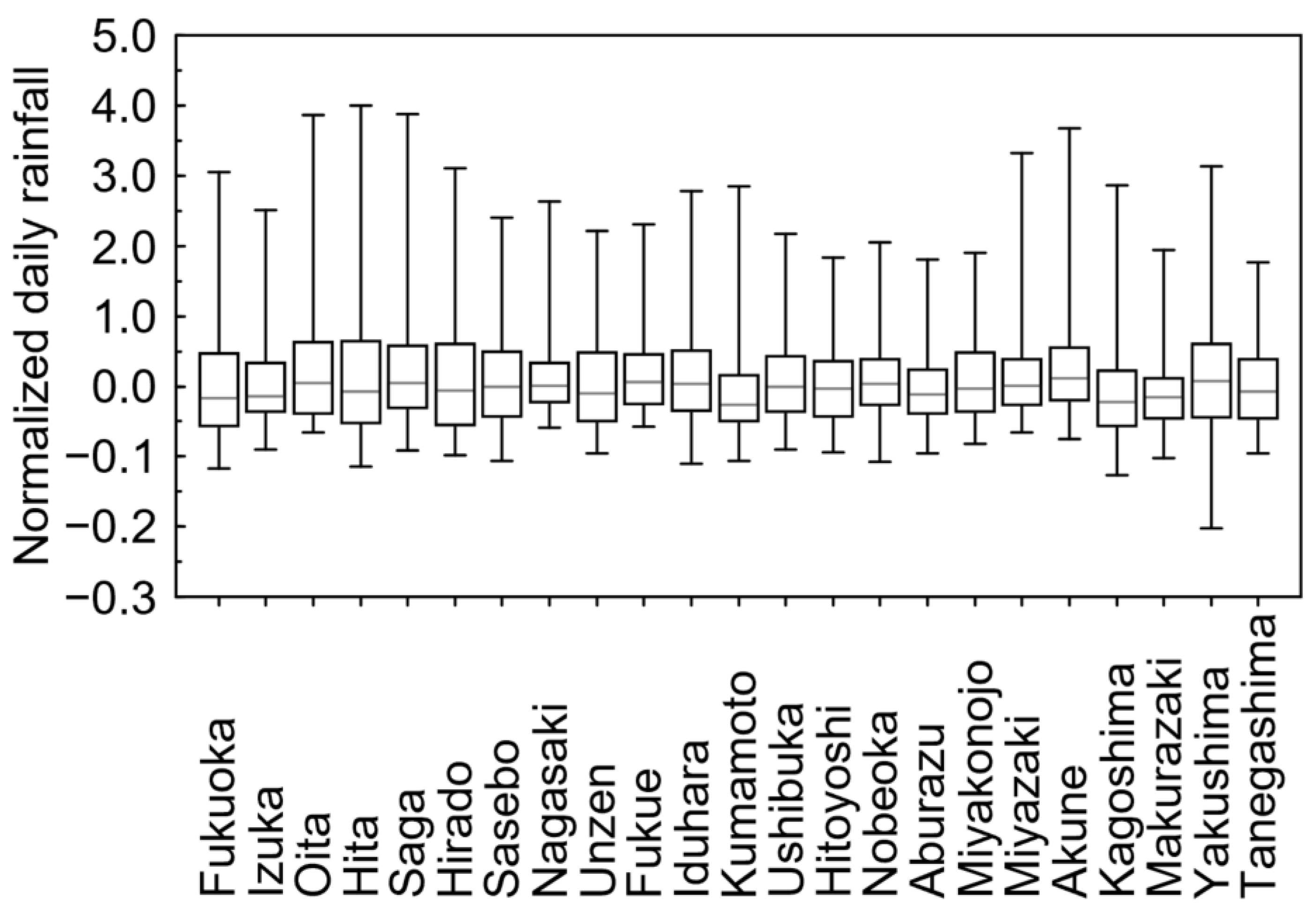
3.3. Normalized Values of Annual Maximum Daily Rainfall at Each Station

Figure 5 shows a boxplot for the normalized values of the annual maximum daily rainfall. As shown in Figure 5, there are wide variations in the data from all stations because the annual maximum value fluctuates by year. On the other hand, there are few differences in the maximum, minimum, interquartile range, and median between stations (Figure 5). As a result, the data exhibited the same probability distributions at all stations and were combined using the station-year method.

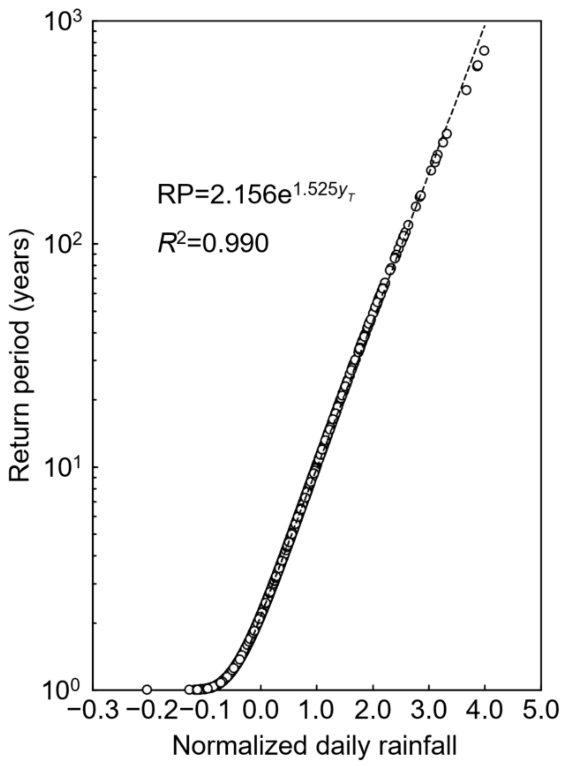
3.4. Relationship between Normalized Daily Rainfall and the RP

Figure 6 shows the quantile–quantile plot (Q-Q plot). As shown in Figure 6, the SLSC value was below the JMA criterion (0.04) [39]. Due to this, the standardized variate and the GEV distribution were a good fit.

Figure 7 shows the relationship between the RP and the normalized values of the annual maximum daily rainfall. As shown in Figure 7, the RP increased exponentially with the increase in the normalized values of the annual maximum daily rainfall when the RP was greater than 1.5 years. Furthermore, this relation indicates that an exponential approximation was obtained by the least-squares method.

$$RP=2.156e^{1.525y_T}$$

(12)

This equation accurately estimates the RP of daily rainfall up to 300 years (Figure 7) by using the 2- and 10-year values at the given stations in Kyushu.

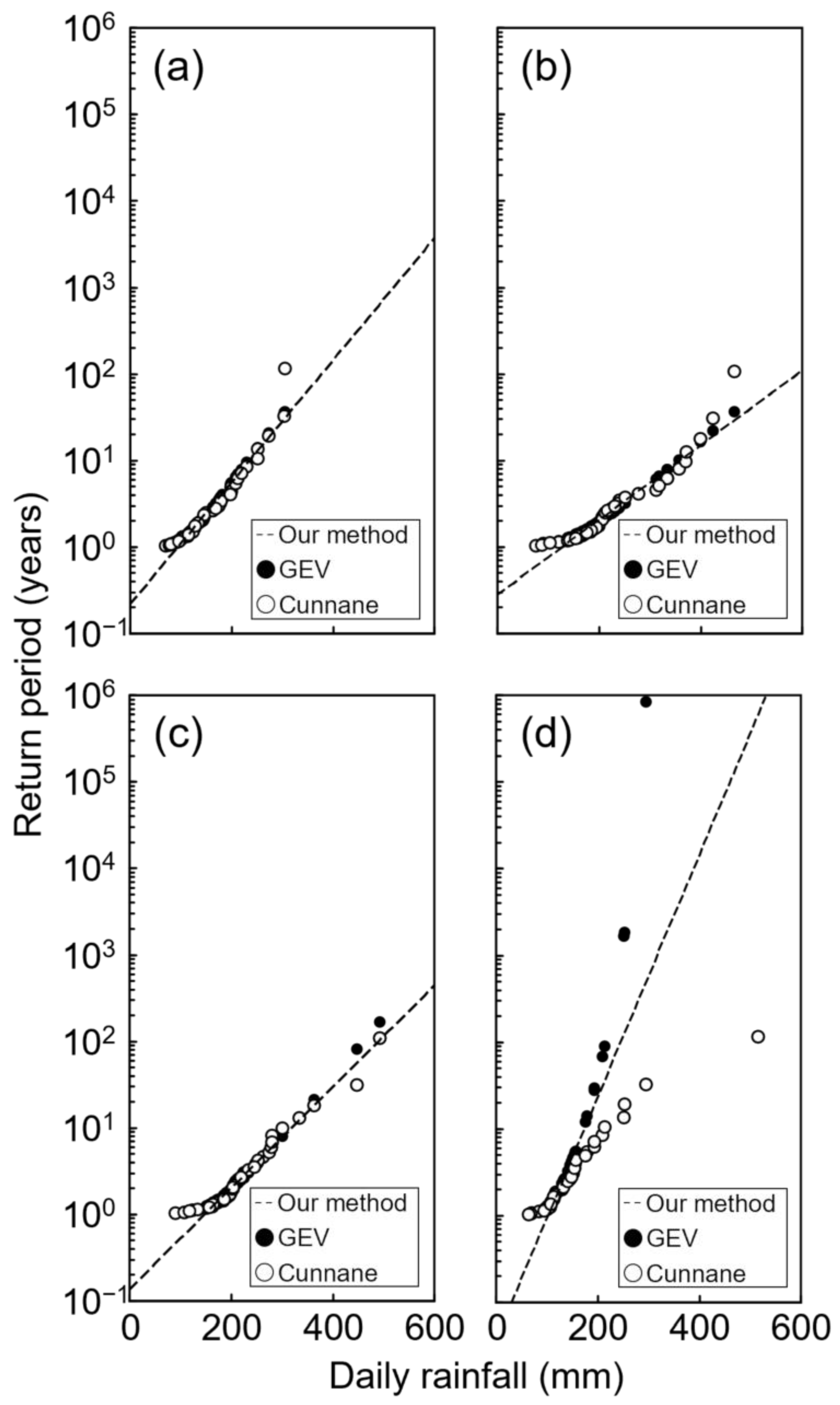
3.5. Verification of Our Method at Short-Record Stations

Figure 8 shows the RP of the annual maximum values for daily rainfall estimated by our method and previous methods. The black and white circle indicates the RP estimated by fitting the GEV distribution and by the plotting position formula, using data from each station, respectively. As shown in Figure 8, the RP estimated by our method was consistent with that calculated by other methods, excluding the AMeDAS Asakura. At the AMeDAS Asakura, the RP might be not consistent with the result of the plotting position formula because a record-breaking regional heavy rainfall event occurred in 2017 [14], and large values for daily rainfall occurred consecutively after periods when the GEV parameters were estimated (Figure 9).

3.6. Usefulness and Limitation of Our Method

Our method estimates the RP of daily rainfall up to 300 years in Kyushu using the 2- and 10-year values at a given station (Figure 7). Extreme daily precipitation is a trigger for floods, landslides, and debris flows (e.g., [43,44]), and estimating them is required to plan, design, and manage hydraulic structures against these disasters [15,16,17,18,45,46]. For example, the Sabo Planning Division, Sabo Department, NILIM, MLIT [46] summarized the methods of the Sabo master plan for preventing damage triggered by debris flows, including driftwood, in Japan. They decided that daily rainfall, corresponding to an exceedance probability of 100 years, can be used to design the scale of measures against debris flow and driftwood [46]. Hence, our method may be applied to estimate the extreme rainfall for developing measures against floods and landslides.

Figure 9. Annual maximum daily rainfall at the AMeDAS Asakura between 1976 and 2020. Gray circles indicate annual maximum value. Bold line indicates Sen’s slope (Hipel and McLeod 1996 [47]; Sen 1968 [48]) (p < 0.05).

Figure 9. Annual maximum daily rainfall at the AMeDAS Asakura between 1976 and 2020. Gray circles indicate annual maximum value. Bold line indicates Sen’s slope (Hipel and McLeod 1996 [47]; Sen 1968 [48]) (p < 0.05).

Extreme daily precipitation is generally estimated by extrapolation because rainfall records at individual stations are often short (e.g., [19]). By contrast, our technique only uses the 2- and 10-year values, which can be calculated by interpolation at many points. Kikuchihara and Suzuki [24] estimated the probability of daily precipitation using a similar approach. Meanwhile, they have not verified their applicability and limitations. In the current study, an empirical dependence (Figure 7) was verified using short-record data (approximately 40 years) at four stations where extreme rainfall was observed. As a result, the RP estimated by our method was consistent with that obtained by other means at most sites (Figure 8a–c); however, it was difficult to apply in stations with an increasing trend in daily rainfall (Figure 8d and Figure 9). This problem may be solved to modify periods for calculating 2- and 10-year values, considering rainfall trends at each station. Overall, we concluded that our method estimates the probability of daily rainfall up to 300 years using data at given stations and contributes to developing strategies for measures against floods and landslides.

4. Conclusions

This study estimated the probability of daily rainfall in the Kyushu region, Japan. The data for the annual maximum values of daily rainfall were obtained from 23 long-record stations and were normalized by quantiles, corresponding to the non-exceedance probability of 50% and 90%. The normalized rainfall at all stations was combined by the station-year method, and the RP was calculated using GEV parameters estimated by the L-moment method. Then, a regression equation linking the normalized values of annual maximum daily rainfall and the RP was obtained; this accurately estimates the RP for up to 300 years. In addition, this relation was verified using the data at short-record stations that observed extreme rainfall events triggering floods and landslides. As a result, the probability of daily precipitation estimated by our approach was consistent with the results of previous techniques. In contrast, our method reduced the uncertainty of extrapolation by using parameters estimated by interpolation. Nevertheless, our method was difficult to apply at sites overserving an increasing trend in daily rainfall; therefore, trends in daily rainfall should be examined to use them. In conclusion, our technique estimates the RP up to 300 years for daily precipitation in Kyushu using data from the given stations, considering outliers. Hence, our findings help to develop measures for floods and landslides.

References

1. Hagon, K.; Turmine, V.; Pizzini, G.; Freebairn, A.; Singh, R. Hazards everywhere-climate and disaster trends and impacts. In World Disasters Report 2020; IFRC, Ed.; IFRC: Geneva, Switzerland, 2020; pp. 34–115. [Google Scholar]
2. Hilker, N.; Badoux, A.; Hegg, C. The Swiss flood and landslide damage database 1972–2007. Nat. Hazards Earth Syst. Sci. 2009, 9, 913–925. [Google Scholar] [CrossRef] [Green Version]
3. Ushiyama, M.; Yokomaku, S. Location characteristics of victims caused by recent heavy rainfall disasters. J. Disaster Inf. Stud. 2013, 11, 81–89, (In Japanese with English Abstract). [Google Scholar] [CrossRef]
4. Hirabayashi, Y.; Mahendran, R.; Koirala, S.; Konoshima, L.; Yamazaki, D.; Watanabe, S.; Kim, H.; Kanae, S. Global flood risk under climate change. Nat. Clim. Chang. 2013, 3, 816–821. [Google Scholar] [CrossRef]
5. McBride, C.M.; Kruger, A.C.; Dyson, L. Changes in extreme daily rainfall characteristics in South Africa: 1921–2020. Weather. Clim. Extrem. 2022, 38, 100517. [Google Scholar] [CrossRef]
6. Shinohara, Y.; Kume, T. Changes in the factors contributing to the reduction of landslide fatalities between 1945 and 2019 in Japan. Sci. Total Environ. 2022, 827, 154392. [Google Scholar] [CrossRef]
7. Matsumoto, J. Heavy rainfalls over east Asia. Int. J. Climatol. 1989, 9, 407–423. [Google Scholar] [CrossRef]
8. Oguchi, T.; Saito, K.; Kadomura, H.; Grossman, M. Fluvial geomorphology and paleohydrology in Japan. Geomorphology 2001, 39, 3–19. [Google Scholar] [CrossRef]
9. Chigira, M. September 2005 rain-induced catastrophic rockslides on slopes affected by deep-seated gravitational deformations, Kyushu, southern Japan. Eng. Geol. 2009, 108, 1–15. [Google Scholar] [CrossRef]
10. Jitousono, T.; Igura, M.; Ue, H.; Ohishi, H.; Kakimoto, T.; Kitou, K.; Koga, S.; Sakai, Y.; Sakasnhima, T.; Shinohara, Y.; et al. The july 2020 rainfall-induced sediment disasters in Kumamoto prefecture, Japan. Int. J. Eros. Control Eng. 2021, 13, 93–100. [Google Scholar] [CrossRef]
11. Sidle, R.C.; Chigira, M. Landslides and debris flows strike Kyushu, Japan. EOS Trans. Am. Geophys. Union 2004, 85, 145–151. [Google Scholar] [CrossRef]
12. Takahashi, T.; de Jong, W.; Kakizawa, H.; Kawase, M.; Matsushita, K.; Sato, N.; Takayanagi, A. New frontiers in Japanese Forest Policy: Addressing ecosystem disservices in the 21st century. Ambio 2021, 50, 2272–2285. [Google Scholar] [CrossRef] [PubMed]
13. Fujiwara, K.; Kawamura, R. Appearance of a Quasi-Quadrennial Variation in Baiu Precipitation in Southern Kyushu, Japan, after the Beginning of This Century. SOLA 2022, 18, 181–186. [Google Scholar] [CrossRef]
14. Imada, Y.; Kawase, H.; Watanabe, M.; Arai, M.; Shiogama, H.; Takayabu, I. Advanced risk-based event attribution for heavy regional rainfall events. NPJ Clim. Atmos. Sci. 2020, 3, 37. [Google Scholar] [CrossRef]
15. Buishand, T.A. Extreme rainfall estimation by combining data from several sites. Hydrol. Sci. J. 1991, 36, 345–365. [Google Scholar] [CrossRef]
16. Koutsoyiannis, D.; Baloutsos, G. Analysis of a Long Record of Annual Maximum Rainfall in Athens, Greece, and Design Rainfall Inferences. Nat. Hazards 2000, 29, 29–48. [Google Scholar] [CrossRef]
17. Overeem, A.; Buishand, A.; Holleman, I. Rainfall depth-duration-frequency curves and their uncertainties. J. Hydrol. 2007, 348, 124–134. [Google Scholar] [CrossRef]
18. Stewart, E.J.; Reed, D.W.; Faulkner, D.S.; Reynard, N.S. The FORGEX method of rainfall growth estimation I: Review of requirement. Hydrol. Earth Syst. Sci. 1999, 3, 187–195. [Google Scholar] [CrossRef] [Green Version]
19. Svensson, C.; Jones, D.A. Review of rainfall frequency estimation methods. J. Flood Risk Manag. 2010, 3, 296–313. [Google Scholar] [CrossRef] [Green Version]
20. Gumbel, E.G. Statistics of Extremes; Columbia University Press: New York, NY, USA, 1958; pp. 1–375. [Google Scholar]
21. Hosking, J.R.M. L-moments: Analysis and estimation of distributions using linear combinations of order statistics. J. Roy. Stat. Soc. Ser. B (Methodol.) 1990, 52, 105–124. [Google Scholar] [CrossRef]
22. Jenkinson, A.F. The frequency distribution of the annual maximum (or minimum) values of meteorological elements. Q. J. R. Meteorol. Soc. 1955, 81, 158–171. [Google Scholar] [CrossRef]
23. Jou, P.H.; Mirhashemi, S.H. Frequency analysis of extreme daily rainfall over an arid zone of Iran using Fourier series method. Appl. Water Sci. 2023, 13, 16. [Google Scholar] [CrossRef]
24. Suzuki, A.; Kikuchihara, H. Method for estimating the return period of annual maximum daily precipitation considering about extreme values. Tenki 1984, 31, 179–189. (In Japanese) [Google Scholar]
25. Clarke-Halstad, K. A statistical method for estimating the reliability of a station-year rainfall-record. EOS Trans. Am. Geophys. Union 1938, 19, 526–529. [Google Scholar] [CrossRef]
26. Clarke-Hafstad, K. Reliability of Station-Year Rainfall-Frequency Determinations. Trans. Am. Soc. Civ. Eng. 1942, 107, 633–652. [Google Scholar] [CrossRef]
27. Hosking, J.R.M.; Wallis, J.R. Regional Frequency Analysis: An Approach Based on L-Moments; Cambridge University Press: Cambridge, UK, 1997; 224p. [Google Scholar]
28. Buishand, T.A. Bivariate extreme-value data and the station-year method. J. Hydrol. 1984, 69, 77–95. [Google Scholar] [CrossRef]
29. Daksiya, V.; Mandapaka, P.V.; Lo, E.Y.M. Effect of climate change and urbanisation on flood protection decisionmaking. J. Flood Risk Manag. 2021, 14, e12681. [Google Scholar] [CrossRef]
30. Olsson, J.; Södling, J.; Berg, P.; Wern, L.; Eronn, A. Short-duration rainfall extremes in Sweden: A regional analysis. Hydrol. Res. 2019, 50, 945–960. [Google Scholar] [CrossRef]
31. Mohammadi, M.; Finnan, J.; Baker, C.; Sterling, M. The potential impact of climate change on oat lodging in the UK and Republic of Ireland. Adv. Meteorol. 2020, 2020, 4138469. [Google Scholar] [CrossRef]
32. Ishikawa, Y.; Shida, T. Mud flow-floating log Disasters in Ichinomia Town, Kumamoto Pref. on July 2nd, 1990. Jpn. Soc. Eros. Control 1990, 43, 63–66. [Google Scholar] [CrossRef]
33. Sassa, K. Mechanisms of Landslide Triggered Debris Flows. In Environmental Forest Science; Sassa, K., Ed.; Springer: Dordrecht, The Netherlands, 1998; pp. 499–518. [Google Scholar] [CrossRef]
34. Yang, H.; Wang, F.; Vilímek, V.; Araiba, K.; Asano, S. Investigation of rainfall-induced shallow landslides on the northeastern rim of Aso caldera, Japan, in July 2012. Geoenviron. Disasters 2015, 2, 20. [Google Scholar] [CrossRef]
35. Kendall, M.G. A new measure of rank correlation. Biometrika 1938, 30, 81–93. [Google Scholar] [CrossRef]
36. Kuzuha, Y.; Tomosugi, K.; Kishii, T. Spatial correlation structure of precipitation. Proc. Hydraul. Eng. 2002, 46, 127–132, (In Japanese with English Abstract). [Google Scholar] [CrossRef]
37. Takara, K. History and Perspectives of Hydrologic Frequency Analysis in Japan. In Pioneering Works on Extreme Value Theory; Hoshino, N., Mano, S., Shimura, T., Eds.; Springer: Singapore, 2021; pp. 113–134. [Google Scholar] [CrossRef]
38. Takasao, T.; Takara, K.; Shimizu, A. A basic study on frequency analysis of hydrologic data in the lake biwa basin. Annu. Disaster Prev. Res. Inst. Kyoto Univ. 1986, 29, 57–171, (In Japanese with English Abstract). Available online: http://hdl.handle.net/2433/71967 (accessed on 22 August 2022).
39. Japan Meteorological Agency. Extreme Weather Risk Map 2006. Available online: https://www.jma.go.jp/jma/press/0703/28b/riskmap18.pdf (accessed on 8 November 2022). (In Japanese).
40. Hazen, A. Storage to be provided in impounding municipal water supply. Trans. Am. Soc. Civ. Eng. 1914, 77, 1539–1640. [Google Scholar] [CrossRef]
41. Cunnane, C. Unbiased plotting positions—A review. J. Hydrol. 1979, 37, 205–222. [Google Scholar] [CrossRef]
42. Fukuoka Regional Headquarters, JMA. Information on Meteorology, Earthquakes, Volcanoes, and Oceans—About Climate. Available online: https://www.jma-net.go.jp/fukuoka/kaiyo/tenkou_main.html (accessed on 8 November 2022). (In Japanese).
43. Chaithong, T. Influence of changes in extreme daily rainfall distribution on the stability of residual soil slopes. Big Earth Data 2022, 1–25. [Google Scholar] [CrossRef]
44. Gaume, E.; Livet, M.; Desbordes, M.; Villeneuve, J.P. Hydrological analysis of the river Aude, France, flash flood on 12 and 13 November 1999. J. Hydrol. 2004, 286, 135–154. [Google Scholar] [CrossRef]
45. Sabo Planning Division Sabo Department, NILIM, MLIT. Manual of Technical Standard for establishing Sabo master plan for debris flow and driftwood. Tech. Note Natl. Inst. Land Infrastruct. Manag. 2016, 904, 1–77. (In Japanese) [Google Scholar]
46. Sabo Planning Division Sabo Department, NILIM, MLIT. Manual of Technical Standard for designing Sabo facilities against debris flow and driftwood. Tech. Note Natl. Inst. Land Infrastruct. Manag. 2016, 905, 1–78. (In Japanese) [Google Scholar]
47. Hipel, K.W.; McLeod, A.I. Time Series Modelling of Water Resources and Environmental Systems; Elsevier: Amsterdam, The Netherlands, 1994; 1012p. [Google Scholar]
48. Sen, P.K. Estimates of the regression coefficient based on Kendall’s tau. J. Am. Stat. Assoc. 1968, 63, 1379–1389. [Google Scholar] [CrossRef]
Figure 1. Location of rainfall stations. White circles and triangles indicate meteorological observatories and AMeDAS, respectively.
Forests 14 00147 g001
Figure 2. Kendall’s τ of annual maximum daily rainfall between stations plotted against distance.
Forests 14 00147 g002
Figure 3. Spatial distribution of the two-year value.
Forests 14 00147 g003
Figure 4. Spatial distribution of the 10-year value.
Forests 14 00147 g004
Figure 5. Boxplots for normalized values of annual maximum daily rainfall at 23 stations. Whiskers of the box show 25th (lower) and 75th (upper) percentile values. The gray line is the median value.
Forests 14 00147 g005
Figure 6. Quantile–quantile plot.
Forests 14 00147 g006
Figure 7. Relationship between normalized values of annual maximum daily rainfall and the RP.
Forests 14 00147 g007
Figure 8. Comparison of RP estimated by the proposed regression equation, RP estimated by the GEV, and RP by the empirical method (Cunnane [39]) at AMeDAS Izumi (a), Morotsuka (b), Aso-Otohime (c), and Asakura (d).
Forests 14 00147 g008