Changes in Forest Conditions in a Siberian Larch Forest Induced by an Extreme Wet Event

Abstract

The taiga forest, a semi-arid and nitrogen-limited ecosystem on permafrost, has changed under extreme wet events. This study aims to understand the changes that occurred in a larch forest in Eastern Siberia after the wet event of 2006–2007. In the summer of 2018, studies were conducted at the Spasskaya Pad Experimental Forest Station near Yakutsk, Russia, where a transect (60 m × 510 m) with 34 plots (30 m × 30 m) was set. It included intact sites and affected sites with different levels of forest damage, owing to the extreme wet event. We observed spatial variations in the normalized difference vegetation index (NDVI) calculated from Landsat satellite-observed data, and the foliar δ¹³C, δ¹⁵N, and C/N (carbon/nitrogen) ratio obtained from the needle samples of 105 mature larch trees. Our results reveal that the affected plots had a lower NDVI than the intact plots, resulting from a difference in tree stand density. In addition, the stand density is suggested to be a controlling factor in the spatial variations in the foliar C/N and δ¹³C values based on their significant relationships with the NDVI in June. We concluded that the larch trees from the regenerating forests in the affected areas have a higher nitrogen level and light availability (relatively low C/N and high δ¹³C) because of the slight competition for resources, owing to a low-stand density. This may lead to further succession of the larch forests after the extreme wet event.

1. Introduction

Extreme precipitation events, such as heavy rainfall and drought, have been observed more frequently and intensively worldwide [1]. These events have different impacts on the hydrological and ecological processes in ecosystems with different soil water availabilities [2]. Although the vegetation responses to drought have been widely studied, the effects of extreme wet events are comparatively less well known. In water-limited regions, the dendrochronological data show increased tree growth after extreme wetness, which offsets the negative impact of drought conditions in previous years [3]. However, in some regions, extreme moist conditions cause a reduction in vegetation productivity [4] and, in severe cases, plant dieback (e.g., [5,6]). The northern regions stand out because extreme events are expected to be more pronounced under Arctic amplification. Therefore, the boreal forest on permafrost, one of the main components of the global carbon cycle, will face changes (e.g., [7]).

The taiga in Northeastern Siberia mainly consists of larch species [8], which grow on permafrost in a continentally dry climate [9]. Under drought conditions, larch trees absorb melted ice water found in the surface soil, which is an important part of permafrost hydrology [10,11]. In addition, plants in the region are nitrogen-limited because of their intense competition with soil microorganisms [12] and the relatively low annual nitrogen (N) supply through mineralization in the soil [13]. The above-mentioned features of the ecosystem make it vulnerable to climatic changes, including extreme events. In Eastern Siberia, near Yakutsk, a large amount of precipitation in 2005 and 2006 led to an increase in soil water content [14], which was the highest in the past 100 years, according to the moisture data reconstructed from the carbon isotope ratio of larch tree rings [15]. Consequently, this event led to a high tree mortality [6] which could negatively impact the forest carbon uptake. Therefore, it is important to understand how this ecosystem changes under extreme wet events, in terms of vegetation production.

One of the approaches is the satellite-derived normalized difference vegetation index (NDVI) as an indicator of the photosynthetically active greenness in order to determine vegetation changes caused by shifts in the environmental parameters. This vegetation index has been identified to correlate with a structural trait, the leaf area index (LAI), i.e., leaf area per unit ground area [16,17,18,19], and fractional vegetation cover (e.g., [20]). It is also considered to be a tool used to estimate a fraction of photosynthetically active radiation (fAPAR) that is absorbed by plants, owing to their relationship [21], which can be converted into net primary production at either the regional or global scale [22]. Because the NDVI can be a proxy for above-ground production, many studies have attempted to compare it with field-observed ecosystem parameters, for example, foliar biochemical traits and isotopic signatures.

The NDVI is based on the red and near-infrared (NIR) radiation reflected from the study area. The red-edge and NIR spectral regions have been shown to be sensitive to leaf nitrogen [23,24], which is one of the most essential biochemical leaf traits. Thus, the foliar nitrogen content (g N/100 g dry leaf weight, %N), as an indicator of nitrogen availability, is suggested to correlate with the vegetation index. Previously, the %N was found to be spatially correlated with the NDVI [25,26,27] and seasonally [28,29] in grasslands and crops for agricultural purposes. The relationship between the NDVI and %N is predominantly positive [25,26,28,29]. At the Siberian taiga–tundra boundary, it has been found that the needle N content of larch trees is an important indicator of nitrogen availability, because it is positively correlated with inorganic nitrogen in soil (ammonium NH₄⁺) [30]. Similarly, Matsushima et al. [31] revealed a positive effect of increased soil N availability after the understory removal and N fertilization experiments on leaf N content in white spruce in Canada. Instead of the nitrogen content, the ratio of foliar carbon to nitrogen content (C/N ratio) has been investigated in many regions in order to estimate the nitrogen use efficiency of plants (e.g., [32,33]).

Another approach involves the leaf isotopic signatures, such as carbon and nitrogen stable isotope compositions (δ¹³C and δ¹⁵N), which are widely applied in order to determine how environmental conditions affect plant physiology. The δ¹³C and δ¹⁵N are calculated by:

δ¹³C (or δ¹⁵N)‰ = (R_sample/R_std − 1) × 1000,

(1)

where R_sample and R_std are isotope ratios (¹³C/¹²C or ¹⁵N/¹⁴N) of the sample and standard, respectively: Vienna Peedee Belemnite (VPDB) for carbon or atmospheric N₂ for nitrogen.

The δ¹³C was found to be sensitive to changes in weather conditions, such as drought and solar radiation [34], resulting in a δ¹³C increase under smaller stomatal conductance and enhanced photosynthesis. After the treatment of a white spruce plantation in Canada, the leaf δ¹³C increased along with the soil N availability (and the leaf N content and the δ¹⁵N) through an enhanced carboxylation rate [31]. The spatial NDVI and δ¹³C have been reported to be negatively correlated in crops [35,36], because a low biomass production was observed in dry areas. Similar results have been shown in regional-scale studies on natural ecosystems, where the spatial variability in leaf carbon isotope composition (or discrimination) is explained by the amount of precipitation in different parts of the study region [37,38,39]. However, in addition to the negative relationship between the NDVI and the leaf δ¹³C in the southern part of the Tibetan Plateau, Guo and Xie [37] also revealed a positive relationship in Northern Tibet; therefore, the NDVI is influenced by the soil. Light conditions also affect the photosynthetic activity and thus the leaf δ¹³C. In Siberian larch trees [33] and most plants [40,41,42], shaded leaves have a lower δ¹³C than sunlit leaves. However, not many papers discussed the relationship between the NDVI and δ¹³C responding to light conditions. So, we expect the correlation between the NDVI and δ¹³C to be an indicator of the environmental variation in soil N and water availability (dry–wet gradient).

The leaf δ¹⁵N serves as an indicator of the nitrogen sources for plants, such as organic or inorganic soil nitrogen and atmospheric nitrogen deposition [43]. In many studies, the foliar δ¹⁵N has been associated with the soil δ¹⁵N (e.g., [44]), that can vary spatially (e.g., [45]) and vertically in depth (e.g., [46]).

The taiga in Eastern Siberia is one of the main biomes in the world because it covers a large area. This forest ecosystem spreads over the permafrost under a continentally dry climate, but the extreme wet event of 2006–2007 changed the forest conditions. The objective of this study was to understand how the forest conditions changed a decade after the event. We investigated the spatial variations in (1) the NDVI and (2) the physiological condition of the larch trees by observing the foliar δ¹³C and δ¹⁵N, and the C/N along a transect including sites unaffected and affected by the wet event.

2. Materials and Methods

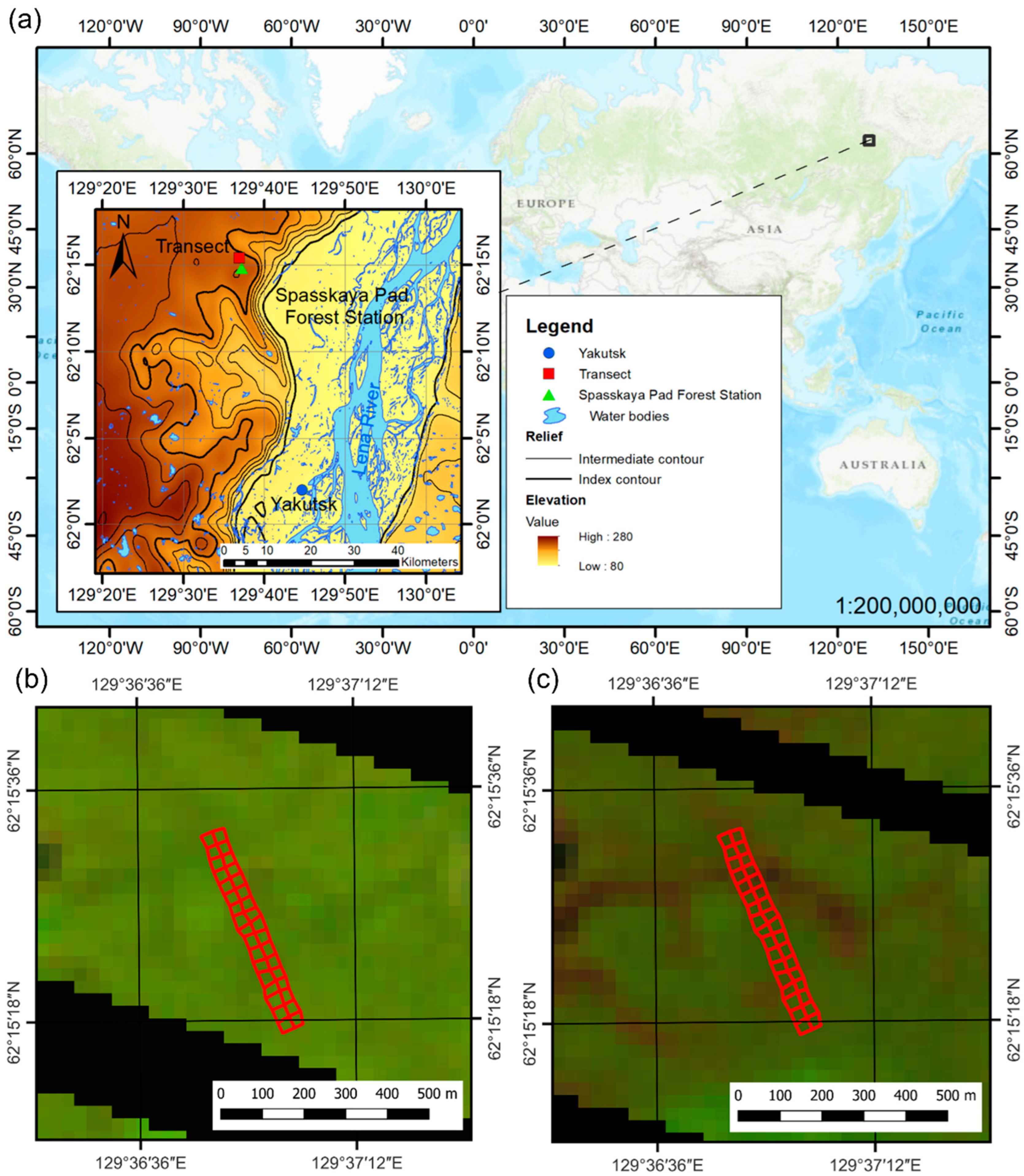
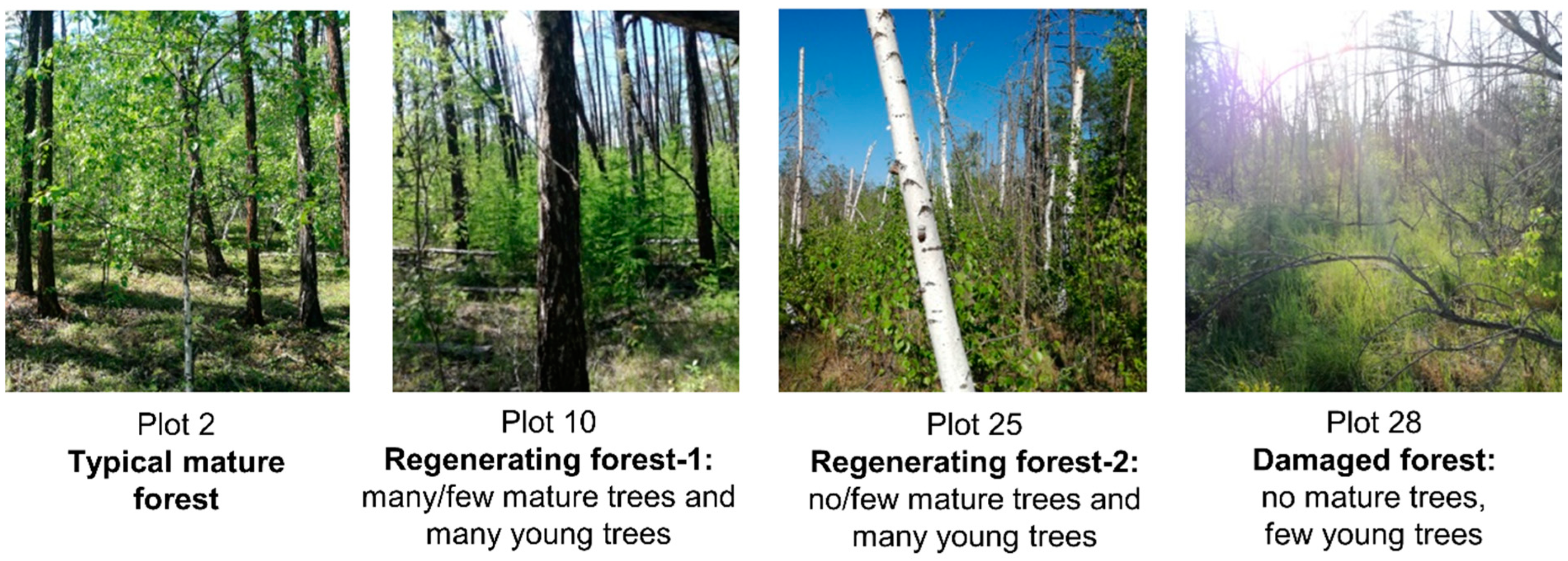
2.1. Study Site and Setting of the Observation Plots

Our observations were conducted in the Spasskaya Pad Experimental Forest (62°15′18″ N, 129°37′08″ E, alt. 220 m a.s.l.), Institute of Biological Problems of Cryolothozone, Siberian Branch of the Russian Academy of Sciences, near Yakutsk, Russia (Figure 1a). This region in Eastern Siberia is characterized by continuous permafrost and an extremely continental climate with a low annual precipitation (238 mm from 1971 to 2000), indicating very dry conditions. The dominant tree species are deciduous larch (Larix cajanderi), and birch (Betula pendula) in the forest gap. There are diverse understory plants, such as dwarf shrubs, Vaccinium vitis-idaea, Arctous alpina, and many species of grasses.

Although this area has a continentally dry climate, an extreme wet event occurred in 2007. The water year precipitation (from October to September) was very large in 2005 (285 mm) and 2006 (340 mm), and the snowfall in the 2006–2007 winter (October to April) was extremely large (106 mm), which was 1.4 times higher than the average (77 mm from 1971 to 2000). This large amount of precipitation caused a high soil moisture level [14], that resulted in a high tree mortality [6]. Following the occurrence of the abnormal wet conditions, the floor vegetation changed to moisture-tolerant grasses and shrubs in some areas, and the stand density of tall trees decreased [6,47,48].

Figure 1b,c shows the vegetation cover (Landsat 7 ETM+ Natural Color Images) 1 km north of the Spasskaya Pad Forest Station before (2006) and after (2008) the extreme wet event, respectively. In order to investigate the long-term effect of the extreme wet event on the forest, in the summer of 2018 (a decade after the event), a 60 m × 510 m transect was set up using wooden pegs and plastic strings, in both intact and affected areas. The transect was divided into 30 m × 30 m plots (in total, 34 plots, red polygons in Figure 1b,c) and these were visually classified based on the forest conditions from the photographs. Four forest types were distinguished along the transect, as shown in Figure 2: typical mature forest (TF; number of plots in the transect, n = 17), regenerating-1 forest (RF-1: many/few mature trees and many young trees; n = 11), regenerating-2 forest (RF-2: few/no mature trees and many young trees; n = 4), and damaged forest (DF: no mature trees, few young trees; n = 2). The first plots discerned as TF, consisted of mature larches, approximately 180 years old with a height of approximately 22 m [49] and these had no visible damage from the wet event. The stand density of the larch trees in the TF measured in August 2018 was 1280 trees ha⁻¹ [50]. The plots discerned as regenerating forest RF-1, had many dead mature larches that formed forest gaps in the overstory where there were a large number of young larches (seedlings and saplings with a height of up to 3 m) and shrubs. In the years following the wet event, larch seeds germinated and formed a large number of young trees in the RF-1. The damaged forest DF, where all mature trees died, was covered predominantly by moisture-tolerant grasses, and there were much smaller numbers of young larches than in the RF-1. The DF plots were located on the depression in a trough and mound topography (shown by a dark-brown color in Figure 1c) and some patches of the DF plots were flooded. The regenerating forest RF-2 plots had a moderate forest condition between the RF-1 and DF. The geographical coordinates (longitude and latitude) of the pegs defining the boundaries of each plot were measured using a handheld GPS (Garmin) with a horizontal accuracy of 3 m in order to estimate the satellite-derived NDVI for the plots.

2.2. NDVI

The atmospherically corrected Landsat 8 Collection 1 Level-2 image products provided by the United States Geological Survey (USGS) website (https://earthexplorer.usgs.gov/, accessed on 3 December 2018) were used to calculate the NDVI. In order to investigate the seasonal variation in the NDVI, we obtained the image products that were photographed between June and September 2018 and georeferenced with the WGS-84 UTM 52N coordinate system corresponding to the location of the study transect. An image product consisted of different spectral bands, including red (R) and near-infrared (NIR) surface reflectance bands with a spatial resolution of 30 m, which were used to compute the raster NDVI with the QGIS software v3.2.2-Bonn (Open Source Geospatial Foundation, Chicago, IL, USA):

NDVI = (NIR − R)/(NIR + R).

(2)

Then, the mean NDVI value was extracted for each transect plot using the zonal statistics function, wherein a transect plot was presented in the QGIS as a polygon vector layer created from the geographical coordinate data. Only the transect plots with pixels showing “clear-terrain, low confidence cloud, and low confidence cirrus” in the Quality Assessment band were used in the analysis. During June–September 2018, the images were taken over 15 days in total, but only five days (4 June, 31 July, 7 August, 23 August, and 17 September) were cloud-free. Therefore, the NDVI on these five observation days were analyzed in this study.

2.3. Larch Needle Sampling and Carbon and Nitrogen Analyses

In the period from late July to early August 2018, one to two tree branches were cut in each plot, from one to four randomly located living mature larch trees, from a height of approximately 6 m in the lower crown, with the use of a pole tree pruner. The needles from each tree were placed in a paper bag and mixed thoroughly. A total of 105 needle samples were collected and oven-dried at 60 °C for 24 h.

The dried needle samples were brought to Hokkaido University, they were powdered with liquid nitrogen, and dried again at 60 °C for 24 h. Each sample was then wrapped in a tin capsule and analyzed for carbon and nitrogen contents and for their isotope compositions using a continuous flow isotope ratio mass spectrometry system consisting of Flash EA 1112 (Thermo Fisher Scientific, Milan, Italy) coupled to Delta V (Thermo Fisher Scientific, Bremen, Germany) via Conflo III interface (Thermo Fisher Scientific, Bremen, Germany). The stable carbon and nitrogen isotopic compositions were reported with the standard δ notation (‰) relative to the VPDB (Vienna Peedee Belemnite) and atmospheric N₂ (air), respectively. The analytical precisions (standard deviation) of the carbon and nitrogen content measurements were better than 0.3% and 0.1%, respectively, and those for the isotopic compositions δ¹³C and δ¹⁵N were 0.1‰.

2.4. Statistical Analysis

For each transect plot, the mean and standard deviation of the needle δ¹³C, δ¹⁵N, and C/N values were calculated. In order to investigate the relationships between the datasets, simple linear regressions were used in R statistics (v3.6.0). The regression models were described by the determination coefficient R² (degree of variance between the observed and fitted values) and p value (statistical significance level).

In order to determine whether the NDVI in the same group (a forest type or the entire transect) on two observation days was different, either the parametric paired Student’s t-test or the non-parametric Wilcoxon signed-rank test was used. If the mean difference between the pairs on two days was normally distributed, according to the Shapiro–Wilk test, the paired t-test was performed; otherwise, the Wilcoxon signed-rank test was used.

In order to define a statistical difference between the means of either the plot NDVI or the individual foliar traits in two different groups (forest types), a parametric unpaired Student’s two-sample t-test was applied in R. This test assumed that two groups of data (forest types) had normal distributions and equal variances, which were checked using the Shapiro–Wilk test and the F-test, respectively. If two normally distributed groups did not have equal variances, Welch’s two-sample t-test was used. If at least one of the two groups was not normally distributed, the non-parametric Wilcoxon rank-sum test was used instead of the t-test.

The statistical significance of the above-mentioned tests and regression model was described based on a level of p < 0.05.

3. Results

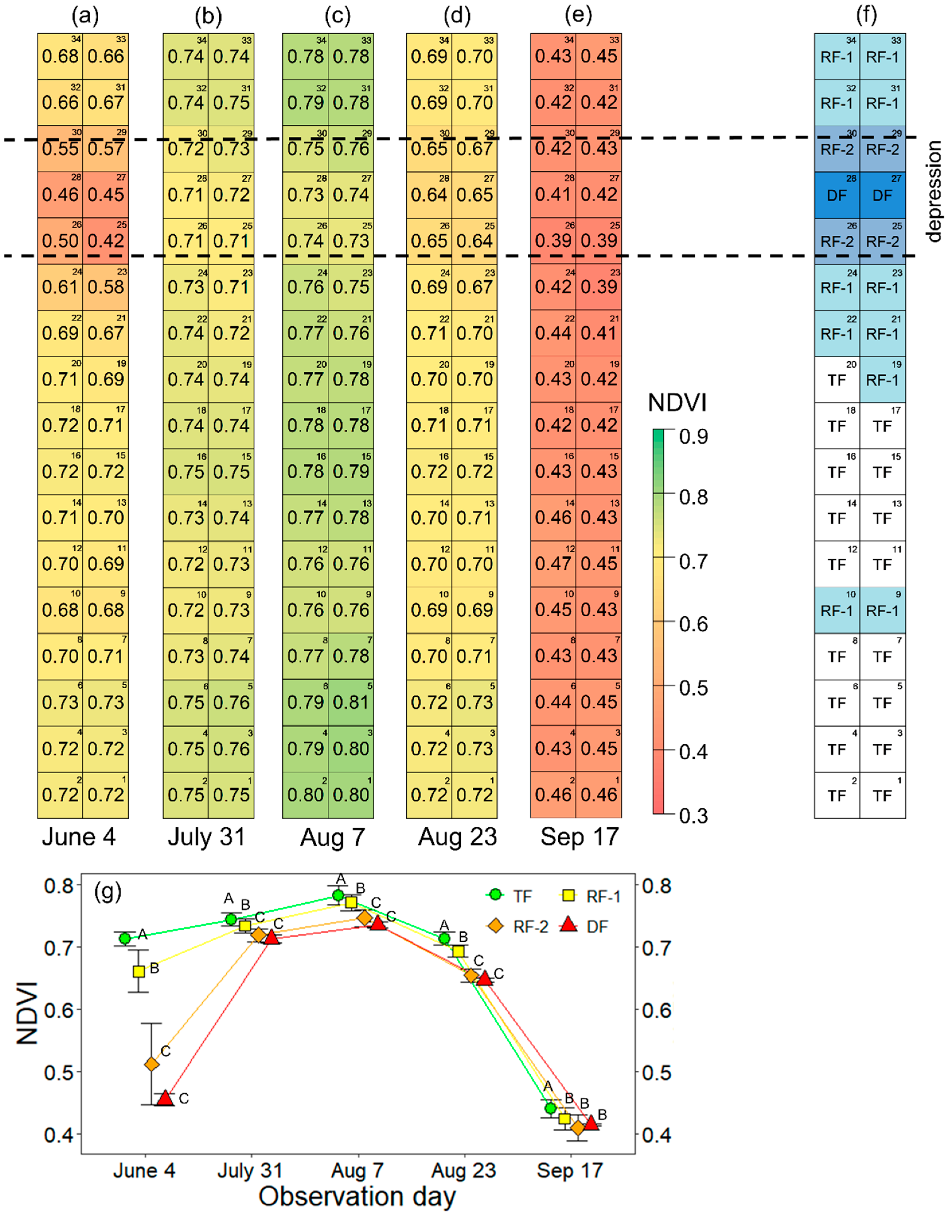
3.1. Seasonal Variation of the NDVI and Forest Condition

Seasonal variations in the NDVI along the transect are shown in Figure 3. The NDVI values of 34 plots varied from 0.42 to 0.73 (0.66 ± 0.09) on 4 June, from 0.71 to 0.76 (0.74 ± 0.01) on 31 July, from 0.73 to 0.81 (0.77 ± 0.02) on 7 August, from 0.64 to 0.73 (0.70 ± 0.02) on 23 August, and from 0.39 to 0.47 (0.43 ± 0.02) on 17 September (Figure 3a–e). The highest values were observed on 7 August and then the NDVI decreased until September. It is important to note that the four forest types showed different NDVI values. The distribution of the forest types along the transect is displayed in Figure 3f. The TF had the highest values, followed by the RF-1, the RF-2, and the DF (Figure 3g). A large difference in the NDVI among the forest types was observed on 4 June: TF, RF-1, RF-2, and DF were 0.71 ± 0.01 (n = 17), 0.66 ± 0.03 (n = 11), 0.51 ± 0.06 (n = 4), and 0.46 ± 0.01 (n = 2), respectively, but the difference was small on 31 July (Figure 3g). Subsequently, the mean NDVI values for the forest types TF, RF-1, RF-2, and DF changed uniformly (Figure 3g). As shown in

Table 1. Comparisons between the mean NDVI in two different forest types on 4 June, 31 July, 7 August, 23 August, and 17 September using two parametric unpaired two-sample tests, such as the classical Student’s equal variances t-test and the Welch unequal variances t-test, and one non-parametric Wilcoxon rank-sum test. The results of these three tests are presented as their significance values (p values).

Day	Forest Types	NDVI (Mean ± SD)	RF-1	RF-2	DF	RF-2 & DF +
4 June	TF	0.71 ± 0.01	<0.001 ***	0.008 **	0.012 *	<0.001 ***
	RF-1	0.66 ± 0.03		0.002 **	0.026 *	<0.001 ***
	RF-2	0.51 ± 0.06			0.533 ns
	DF	0.46 ± 0.01
	RF-2 & DF	0.49 ± 0.06
31 July	TF	0.74 ± 0.01	0.02 *	<0.001 ***	0.012 *	<0.001 ***
	RF-1	0.73 ± 0.01		0.03 *	0.051 ′	0.006 **
	RF-2	0.72 ± 0.01			0.533 ns
	DF	0.71 ± 0.01
	RF-2 & DF	0.72 ± 0.01
7 August	TF	0.78 ± 0.01	0.04 *	<0.001 ***	0.012 *	<0.001 ***
	RF-1	0.77 ± 0.01		0.006 **	0.026 *	<0.001 ***
	RF-2	0.75 ± 0.01			0.533 ns
	DF	0.74 ± 0.00
	RF-2 & DF	0.74 ± 0.01
23 August	TF	0.71 ± 0.01	<0.001 ***	<0.001 ***	0.012 *	<0.001 ***
	RF-1	0.69 ± 0.01		0.002 **	0.026 *	<0.001 ***
	RF-2	0.65 ± 0.01			0.533 ns
	DF	0.65 ± 0.00
	RF-2 & DF	0.65 ± 0.01
17 September	TF	0.44 ± 0.01	0.02 *	0.003 **	0.012 *	<0.001 ***
	RF-1	0.42 ± 0.02		0.21 ns	0.231 ns	0.17 ns
	RF-2	0.41 ± 0.02			1 ns
	DF	0.42 ± 0.00
	RF-2 & DF	0.41 ± 0.02

Bold font indicates a significant difference between the NDVI means. Significance levels were flagged as the following: ′ p < 0.1, * p < 0.05; ** p < 0.01, *** p < 0.001, ns—not significant. ⁺ Because of the small sample sizes in the RF-2 (n = 4) and DF (n = 2) and the statistically insignificant difference in the NDVI between them on each observation day, the RF-2 and DF were brought together as one group (n = 6).

, the statistical tests revealed the highest NDVI in the TF and the lowest NDVI in the RF-2 and DF; the difference between the RF-2 and DF was statistically insignificant. The RF-1 was between the highest (TF) and lowest (RF-2 and DF) in June, July, and August (Table 1).

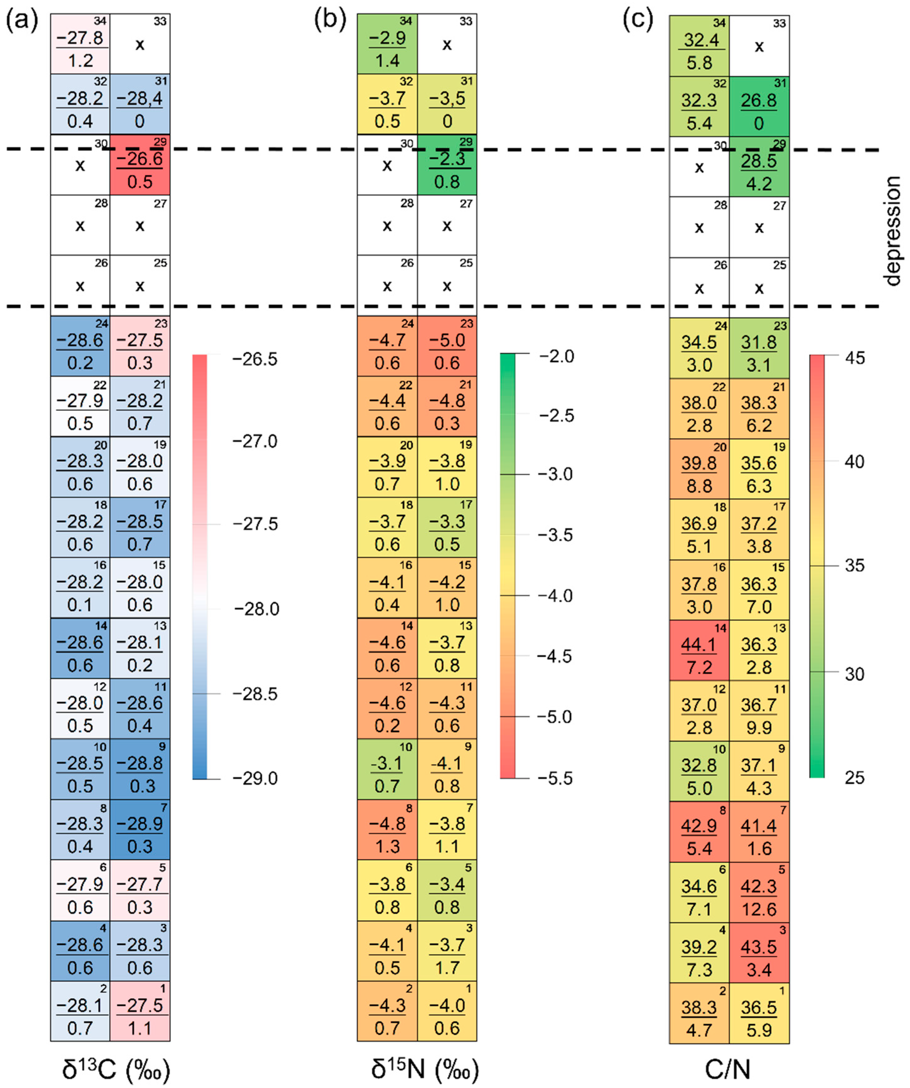
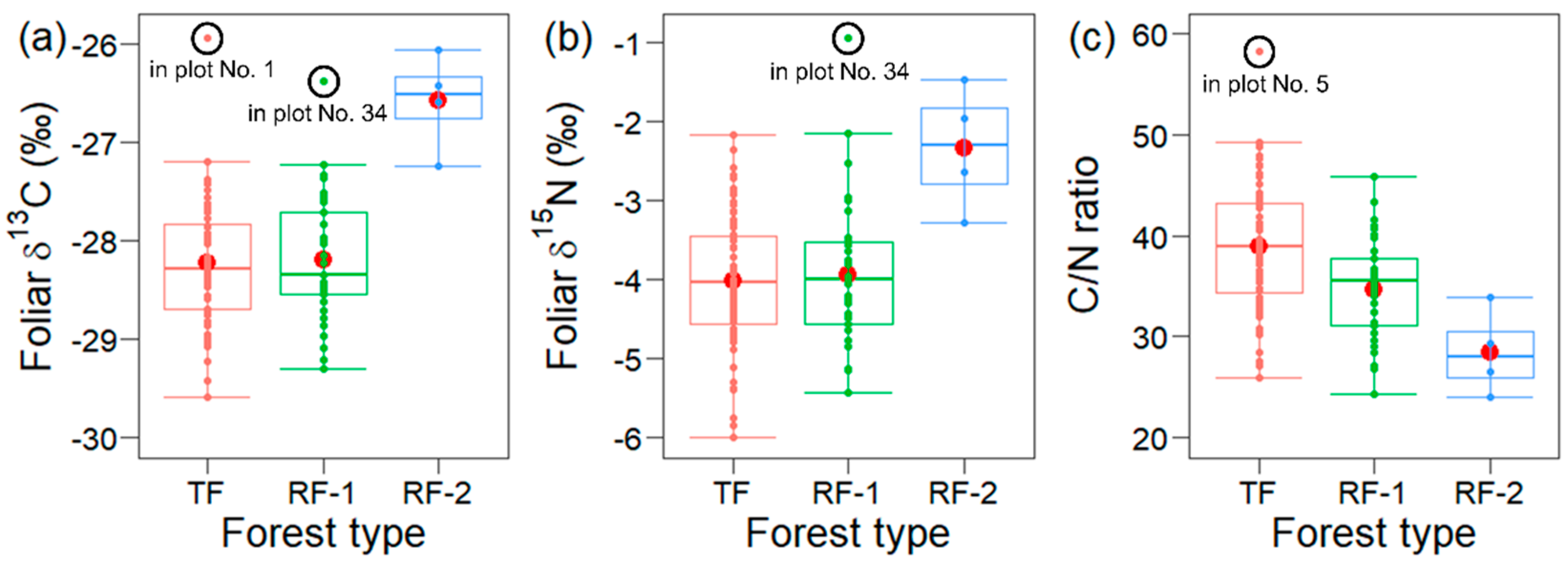
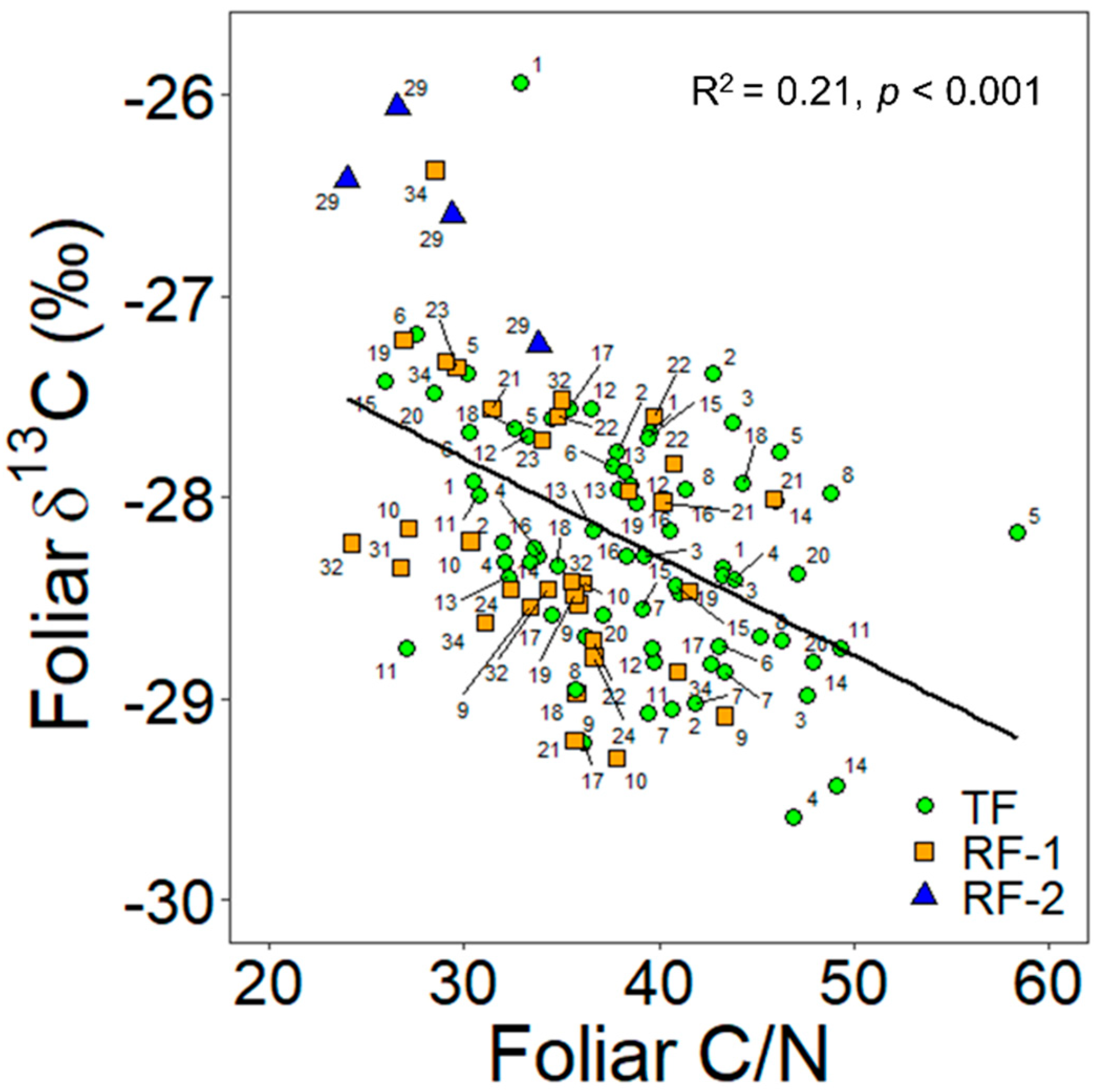
3.2. Spatial Variations in the Larch Foliar Traits

Spatial variations in the foliar δ¹³C and δ¹⁵N values and the C/N ratios along the transect are shown in Figure 4. Six of the 34 plots had no data because no mature trees or other trees were available for sampling using the pole tree pruner. The foliar δ¹³C averaged for all samples was −28.2 ± 0.7‰ (n = 105). Among the plots, the lowest δ¹³C was found in the TF plot No. 7 (−28.9 ± 0.3‰, n = 4), and the highest was in the RF-2 plot No. 29 (−26.6 ± 0.5‰, n = 4) (Figure 4a). As seen in Figure 5a, when comparing the forest types, the mean δ¹³C of the RF-2 (−26.6 ± 0.5‰, n = 4) was higher than that of the TF (−28.2 ± 0.6‰, n = 68) and the RF-1 (−28.2 ± 0.6‰, n = 33), but, according to the Student’s t-tests, no significant difference was observed among the TF, RF-1, and RF-2.

As shown in Figure 5a, there were several outliers. Relatively high δ¹³C values of individual trees were observed not only in the RF-2 plot but also in the TF plot No. 1 (−25.9‰) and the RF-1 plot No. 34 (−26.4‰). We describe these data later in the Discussion section.

The foliar δ¹⁵N value averaged for all samples was −3.9 ± 0.9‰ (n = 105). The mean δ¹⁵N of the plots ranged from −5.0 ± 0.6 (RF-1 plot No. 23) to −2.3 ± 0.8‰ (RF-2 plot No. 29) (Figure 4b). Among the forest types, the mean δ¹⁵N values were statistically insignificant, although the TF (−4.0 ± 0.8‰, n = 68) and RF-1 (−3.9 ± 0.9‰, n = 33) had a lower δ¹⁵N than the RF-2 (−2.3 ± 0.8‰, n = 4) (Figure 5b).

The foliar C/N ratio showed that the mean value of 37.2 ± 6.4 (n = 105) for all samples, ranging from 24.0 to 58.3 was observed in trees in the RF-2 plot No. 29 and the TF plot No. 5, respectively. Among the forest types, no significant difference in the C/N was observed, but the C/N ratio in the TF (38.9 ± 6.3, n = 68) was higher than that in the RF-1 (34.7 ± 5.2, n = 33), and the RF-2 (28.4 ± 4.2, n = 4) showed the lowest C/N (Figure 4c and Figure 5c).

The C/N and δ¹³C values for each tree sample were found to be linearly related at a significant level, but with much variation (R² = 0.18, p < 0.05; Figure 6). The other foliar traits showed no significant relationships.

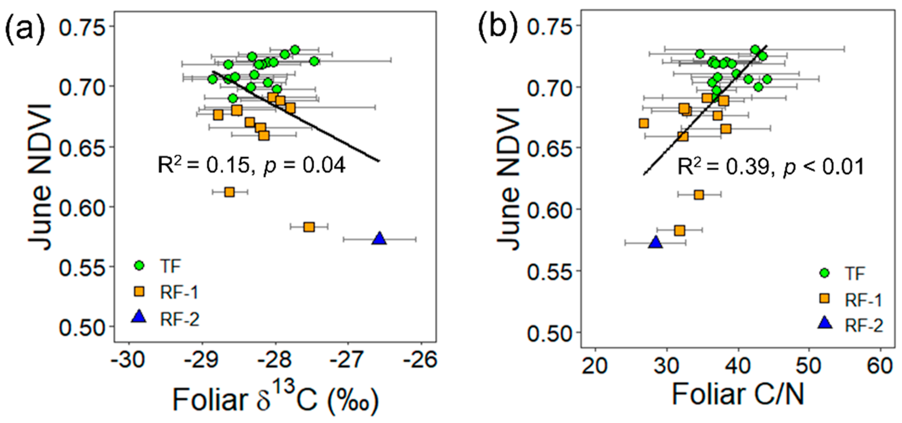
3.3. Relationships between the NDVI and the Foliar Traits

The statistical parameters that describe the linear regression models between the foliar traits and the NDVI are tabulated in

Table 2. Linear regression models between the plot NDVI which were calculated from the Landsat-8 OLI images on 4 June, 31 July, 7 August, 23 August, and 17 September (independent variables) and the plot-averaged δ¹³C, δ¹⁵N, and C/N of the larch needles sampled (dependent variable x). Models were described by the R-squared and p value. Number of plots used in the models is 28 out of 34: with the TF (n = 17), the RF-1 (n = 10), and the RF-2 (n = 1).

Day	Foliar δ13C (‰)			Foliar δ13N (‰)			Foliar C/N
	NDVI = b1x + b0	R2	p	NDVI = b1x + b0	R2	p	NDVI = b1x + b0	R2	p
4 June	−0.240x − 0.033	0.15	0.04 *		<0.01	0.93 ns	0.006x + 0.465	0.39	<0.01 **
31 July		0.01	0.64 ns	0.007x + 0.769	0.16	0.04 *		0.04	0.30 ns
7 August		0.01	0.64 ns		0.10	0.11 ns		0.06	0.20 ns
23 August		0.06	0.20 ns		0.00	1.00 ns	0.002x + 0.618	0.39	<0.01 **
17 September		0.00	0.90 ns		0.01	0.63 ns	0.002x + 0.376	0.15	0.04 *

Bold font indicates a significant relationship. Significance levels (p values) were flagged as * p < 0.05, ** p < 0.01, ns—not significant.

. The NDVI on 4 June was linearly related to the δ¹³C and the C/N (Figure 7). The δ¹³C showed a significant negative relationship with the 4 June NDVI, but there was significant variation in the δ¹³C (R² = 0.15, p < 0.05; Figure 7a). The 4 June NDVI values showed a significant increasing trend with the plot C/N ratio (R² = 0.39, p < 0.01) or a decreasing trend with the N content (Figure 7b). In addition, the C/N was positively correlated with the NDVI on 23 August (R² = 0.39, p < 0.01) and 17 September (R² = 0.15, p < 0.05).

4. Discussion

4.1. Plant Phenology and Seasonality of the Ecosystem of Each Forest Type

One of the purposes of this study, was to identify whether the vegetation productivity varied between the four forest types after the damage caused by the wet event, during the growing season. Unfortunately, the number of observation days for the NDVI was limited by sparse data acquisition (every 16 days) and cloud-contaminated images. As a result, only five days’ (4 June, 31 July, 7 August, 23 August, and 17 September) worth of data was available in order to interpret the general trends in the NDVI for better understanding the phenology.

The transect NDVI increased from 4 June to 7 August, and the seasonal peak was reached on 7 August for all forest types (Figure 3g). The maximum greenness in both the intact and affected areas at the beginning of August implied that the highest foliar biomass production of the above-ground vegetation was as a result of its growth. The timing and magnitude of the peak NDVI in an ecosystem can vary spatially and annually. Previously, the phenology of Siberian forests was found to be controlled by precipitation and air temperature, and the peak NDVI was determined to occur usually in July [51]. However, in our case, it was difficult to determine the date of the seasonal peak because of the sparse data acquisition. The NDVI peak in 2018 could have been reached earlier. Following the vegetation green-up, the NDVI subsequently decreased owing to leaf senescence (yellowing) (Figure 3g).

On all observation days, the NDVI values were the highest in the TF and decreased due to the damage by the wet event, although statistically similar (insignificant), the RF-2 and DF data were the lowest (Figure 3g). The descending order of the NDVI from the intact (TF) to the more affected areas can be explained by the differences in the tree stand density. Although a typical forest is composed of a large number of larches making up the dense canopy, the damaged forest has no mature trees. In turn, the regenerating forests RF-1 and RF-2 had gaps in the forest canopy, where many trees died after the wet event. The positive effect of the stand density on the NDVI can be associated with a positive relationship between the NDVI and the LAI [52,53]. A typical larch forest in the intact area is supposed to have a higher foliar biomass production than other forest types, with a lower number of trees in the affected area. However, several studies conducted in northern boreal regions showed a negative relationship between the NDVI and the attributes of the above-ground biomass. In Siberian larch forests, Loranty et al. [54] found that the mean seasonal NDVI was lower at sites with a higher overstory stand density. In Canadian permafrost peatlands covered by black spruce and larch, both the stand density and basal area were negatively correlated with the peak NDVI [55]. In those studies, this implicit phenomenon could be explained by shadowing both the understory and lower part of the crowns in dense conifer stands, which decreases the NDVI values (e.g., [56]). However, in our case, the foliar biomass of the forest canopy was the main factor controlling the spatial variation in the NDVI.

The difference in the NDVI between the highest (TF) and the lowest (DF) forest types was the largest on 4 June and then significantly decreased by 31 July, after which it remained small. As a result, the increase in the NDVI from 4 June to 31 July was smallest in the TF and largest in the DF (Figure 3g). This can be associated with the phenological features of the above-ground vegetation for each type. The intact and affected areas differed in the ratio of the overstory and the surface vegetation exposed to radiation. A small increase in the NDVI in the TF was mainly caused by the growth of needles and shoots of mature larches, whereas a large increase in the DF was induced by the growth of grasses, shrubs, and young larches. In turn, the increases in the NDVI in the RF-1 and RF-2 resulted from the phenology of both the forest canopy and surface vegetation. Therefore, the production of surface vegetation, such as shrubs and grasses, is high during this period and causes a higher NDVI. Chen and Cihlar [16] reported a similar finding when they found a stronger relationship between the NDVI and the overstory LAI in open boreal conifer stands in late spring than in mid-summer. Because the understory and floor vegetation greatly contribute to the NDVI in the middle of the growing season, it was reasonable to use the NDVI in early summer in order to investigate the spatial variation in the above-ground production of the overstory.

Thus, throughout the growing season, the vegetation in the intact (TF) and affected (RF-1, RF-2, and DF) areas varied in phenology. At the beginning of the growing season, the large difference in the NDVI between the areas was associated with the mature larch tree stand density: the NDVI was higher in the intact area with a dense forest canopy than in the affected area. However, afterwards, the difference was smaller on the subsequent observation days because the surface vegetation in the gaps of the forest canopy in the affected area grew and showed a high level of greenness. The maximum production in both areas was reached at the same time, at the beginning of August. The NDVI then decreased uniformly because of the leaf senescence.

4.2. Forest Condition after the Damage by the Wet Event

In order to understand the physiological responses of larch trees after the wet event, we compared the needle parameters, such as the δ¹³C, the δ¹⁵N, and the C/N, among the forest types, but the results were not statistically significant. These results could be derived from the sample size; namely, the much smaller sample sizes from the RF-1 (n = 33) and RF-2 (n = 4) than from the TF (n = 66) may have produced non-significant relationships.

In our study, as seen in Figure 4a and Figure 7a, the highest δ¹³C values in the transect were found in the RF-2 plot No. 29 and the RF-1 plot No. 23 near the depression, where the tree stand density seemed to significantly decrease after the extreme wet event. There are two potential reasons for these high δ¹³C values. The first was that the high δ¹³C was caused by water logging [57], such as the extreme wet event that occurred in 2007, and the second was because of the light condition. For the first reason, during waterlogging pot experiments, Li and Sugimoto [57] reported an increase in foliar δ¹³C values for the larch trees Larix gmelini. However, such high δ¹³C values were photosynthesized only during water logging, and there was no water in the RF-1 or RF-2. In addition, according to the C/N data from the RF-1 and RF-2, there were favorable conditions in terms of the nitrogen availability (low C/N ratio or high N content). Therefore, the high foliar δ¹³C was caused by the second reason; that is, the high δ¹³C in the low-density stand can be explained by a higher light availability than in the dense stands. The laboratory observations, which were conducted by Ehleringer et al. [41], support that the light level is the environmental parameter most likely responsible for the changes in the intercellular CO₂ levels that, consequently, lead to a higher δ¹³C.

The results of the vertical gradients in the δ¹³C have been reported in many studies [40,41,42]. In dense stands, the leaves in the lower part of the tree crown have a lower δ¹³C than those in the upper part, owing to shading. Thus, the regenerating forest stands with a low number of trees are supposed to be more exposed to light, resulting in higher δ¹³C values than those in typical forests with a large number of trees.

It is necessary to mention that high δ¹³C values were observed not only in regenerating forests but also in typical forests (Figure 5a). As shown in Figure 5a, the δ¹³C of the trees from the TF plot No. 1 (−25.9‰) and the RF-1 No. 34 (−26.4‰) was unusually high (outliers). The reason for this high δ¹³C could be the same as that from the RF-2 because the C/N ratio of these trees was relatively low (32.9 and 28.5, respectively), indicating a high nitrogen availability. In addition to these outlier data, some of the trees from the TF had a relatively high δ¹³C, but there was a high C/N ratio (e.g., −28.2‰ and 58.3 for the δ¹³C and the C/N in plot No. 5, Figure 6). This result indicates that the trees were under dry conditions.

The C/N averaged for each forest type varied: the TF was the highest, the RF-1 was intermediate, and the lowest value was observed in the RF-2. As described before, the NDVI was similarly different among the TF, RF-1, and RF-2 (Figure 3g); therefore, the plot-averaged C/N was positively correlated with the NDVI at different phenological stages in early June (leaf development) and at the end of August and September (senescence) (see Table 2). Thus, the C/N varied significantly among the forest types, which means that forest density could affect the nitrogen uptake by larch trees. Thus, the low foliar C/N values, that is, the high N content observed in the plots with the regenerating forest, indicate a higher nitrogen availability for larch trees. This was an unexpected result because the nitrogen uptake was hypothesized to be limited in wet areas, owing to intensive competition between plant roots and soil communities. Previously, the spatial NDVI and mass-based N content were found to be negatively correlated only in grasslands [27]. In Bromus inermis prairies, such negative relationships were found at the beginning and at the end of the growing season, which are presumably controlled by tallgrass regrowth after grazing and senescence, respectively [27]. We expected that the N availability for a tree in the affected plots would be lower than that in the plots with a typical forest because of the inactive nitrogen production in wet soil. However, our results show a higher N availability for one mature tree in the affected forest, owing to slight competition among trees. In addition, the larch trees in the affected areas can be well supplied with water, which increases the nitrogen uptake. Our results regarding the foliar nitrogen isotopic composition were ambiguous. The plot δ¹⁵N was not dependent on the June NDVI, which was considered to represent the tree stand density, but there was a significant positive relationship between the plot δ¹⁵N and the NDVI in July. Generally, individual trees exhibited large variations in the foliar δ¹⁵N values. The high variability observed in our study demonstrates the spatial heterogeneity of the soil along the transect.

As a result, we found spatial variations in the NDVI, the foliar δ¹³C, and the C/N depending on forest conditions formed after the wet event. Generally, a level of forest damage in our study site was controlled by microtopographical conditions [6], thereby the highest tree mortality was observed on the topographical depression in the northern part of the transect (DF). Moreover, soil properties, such as water retention and porosity [6], could have an influence on the formation of the forest types and, consequently, on the variations in the NDVI, the foliar δ¹³C, and the C/N.

5. Conclusions

We studied the spatial variations in the NDVI and the leaf-level indicators of the physiological response of the larch forest in Eastern Siberia 10 years after the extreme wet event. In the current study, the stand density (number of mature trees per unit area) seemed to be an important factor controlling the changes in the NDVI. In the affected areas, i.e., the regenerating (RF) and damaged (DF) forests, a high tree mortality caused a lower NDVI on each observation day than that in the intact forest (TF). The difference in the NDVI between the TF and the DF (and the RF) was great in June, but in August (seasonal maximum NDVI) the difference was small because of a high production of water-tolerant grasses in the DF (and the RF). The larch trees in the RF (lower June NDVI) had higher light (higher foliar δ¹³C) and nitrogen (lower foliar C/N) availabilities because of a reduced competition for light and soil nitrogen among trees. Such favorable conditions and the presence of a large number of young larch trees may lead to further succession of the RF after the extreme wet event. In order to better understand the effects of wet events in otherwise usually dry forests, long-term observations of the DF should be continued. In addition, observations of forest productivity and area-based nitrogen availability and investigation of historical changes in the NDVI can be useful in order to understand forest conditions.

References

1. Douville, H.; Raghavan, K.; Renwick, J.; Allan, R.P.; Arias, P.A.; Barlow, M.; Cerezo-Mota, R.; Cherchi, A.; Gan, T.Y.; Gergis, J.; et al. Water Cycle Changes. In Climate Change 2021: The Physical Science Basis. Contribution of Working Group I to the Sixth Assessment Report of the Intergovernmental Panel on Climate Change; Masson-Delmotte, V., Zhai, P., Pirani, A., Connors, S.L., Péan, C., Berger, S., Caud, N., Chen, Y., Goldfarb, L., Gomis, M.I., et al., Eds.; Cambridge University Press: Cambridge, UK; New York, NY, USA, 2021; pp. 1055–1210. [Google Scholar]
2. Knapp, A.K.; Beier, C.; Briske, D.D.; Classen, A.T.; Luo, Y.; Reichstein, M.; Smith, M.D.; Smith, S.D.; Bell, J.E.; Fay, P.A.; et al. Consequences of More Extreme Precipitation Regimes for Terrestrial Ecosystems. Bioscience 2008, 58, 811–821. [Google Scholar] [CrossRef]
3. Jiang, P.; Liu, H.Y.; Piao, S.L.; Ciais, P.; Wu, X.C.; Yin, Y.; Wang, H.Y. Enhanced growth after extreme wetness compensates for post-drought carbon loss in dry forests. Nat. Commun. 2019, 10, 195. [Google Scholar] [CrossRef] [PubMed]
4. Heisler-White, J.L.; Blair, J.M.; Kelly, E.F.; Harmoney, K.; Knapp, A.K. Contingent productivity responses to more extreme rainfall regimes across a grassland biome. Glob. Chang. Biol. 2009, 15, 2894–2904. [Google Scholar] [CrossRef]
5. Rozas, V.; Garcia-Gonzalez, I. Too wet for oaks? Inter-tree competition and recent persistent wetness predispose oaks to rainfall-induced dieback in Atlantic rainy forest. Glob. Planet. Chang. 2012, 94–95, 62–71. [Google Scholar] [CrossRef] [Green Version]
6. Iwasaki, H.; Saito, H.; Kuwao, K.; Maximov, T.C.; Hasegawa, S. Forest decline caused by high soil water conditions in a permafrost region. Hydrol. Earth Syst. Sci. 2010, 14, 301–307. [Google Scholar] [CrossRef] [Green Version]
7. Richardson, A.D.; Keenan, T.F.; Migliavacca, M.; Ryu, Y.; Sonnentag, O.; Toomey, M. Climate change, phenology, and phenological control of vegetation feedbacks to the climate system. Agric. For. Meteorol. 2013, 169, 156–173. [Google Scholar] [CrossRef]
8. Abaimov, A.P.; Lesinski, J.A.; Martinsson, O.; Milyutin, L.I. Variability and Ecology of Siberian Larch Species; Reports; Swedish University of Agricultural Sciences, Departament of Silviculture: Umeå, Sweden, 1998; Volume 43, p. 123. [Google Scholar]
9. Archibold, O.W. The coniferous forests. In Ecology of World Vegetation; Springer: Dordrecht, The Netherlands, 1995; pp. 238–279. [Google Scholar] [CrossRef]
10. Sugimoto, A.; Yanagisawa, N.; Naito, D.; Fujita, N.; Maximov, T.C. Importance of permafrost as a source of water for plants in east Siberian taiga. Ecol. Res. 2002, 17, 493–503. [Google Scholar] [CrossRef]
11. Sugimoto, A.; Naito, D.; Yanagisawa, N.; Ichiyanagi, K.; Kurita, N.; Kubota, J.; Kotake, T.; Ohata, T.; Maximov, T.C.; Fedorov, A.N. Characteristics of soil moisture in permafrost observed in East Siberian taiga with stable isotopes of water. Hydrol. Process. 2003, 17, 1073–1092. [Google Scholar] [CrossRef]
12. Popova, A.S.; Tokuchi, N.; Ohte, N.; Ueda, M.U.; Osaka, K.; Maximov, T.C.; Sugimoto, A. Nitrogen availability in the taiga forest ecosystem of northeastern Siberia. Soil Sci. Plant Nutr. 2013, 59, 427–441. [Google Scholar] [CrossRef] [Green Version]
13. Matsuura, Y.; Hirobe, M. Soil carbon and nitrogen, and characteristics of soil active layer in Siberian permafrost region. In Permafrost Ecosystems. Siberian Larch Forests; Osawa, A., Zyryanova, O.A., Matsuura, Y., Kajimoto, T., Wein, R.W., Eds.; Springer: Dordrecht, The Netherlands, 2010; pp. 149–163. [Google Scholar] [CrossRef]
14. Sugimoto, A. Stable Isotopes of Water in Permafrost Ecosystem. In Water-Carbon Dynamics in Eastern Siberia. Ecological Studies (Analysis and Synthesis); Ohta, T., Hiyama, T., Iijima, Y., Kotani, A., Maximov, T., Eds.; Springer: Singapore, 2019; Volume 236. [Google Scholar]
15. Tei, S.; Sugimoto, A.; Yonenobu, H.; Yamazaki, T.; Maximov, T.C. Reconstruction of soil moisture for the past 100 years in eastern Siberia by using delta C-13 of larch tree rings. J. Geophys. Res.-Biogeosci. 2013, 118, 1256–1265. [Google Scholar] [CrossRef]
16. Chen, J.M.; Cihlar, J. Retrieving leaf area index of boreal conifer forests using landsat TM images. Remote Sens. Environ. 1996, 55, 153–162. [Google Scholar] [CrossRef]
17. Wang, Q.; Adiku, S.; Tenhunen, J.; Granier, A. On the relationship of NDVI with leaf area index in a deciduous forest site. Remote Sens. Environ. 2005, 94, 244–255. [Google Scholar] [CrossRef]
18. Gamon, J.A.; Field, C.B.; Goulden, M.L.; Griffin, K.L.; Hartley, A.E.; Joel, G.; Penuelas, J.; Valentini, R. Relationships between NDVI, canopy structure, and photosynthesis in 3 Californian vegetation types. Ecol. Appl. 1995, 5, 28–41. [Google Scholar] [CrossRef] [Green Version]
19. Juszak, I.; Erb, A.M.; Maximov, T.C.; Schaepman-Strub, G. Arctic shrub effects on NDVI, summer albedo and soil shading. Remote Sens. Environ. 2014, 153, 79–89. [Google Scholar] [CrossRef] [Green Version]
20. Blok, D.; Schaepman-Strub, G.; Bartholomeus, H.; Heijmans, M.; Maximov, T.C.; Berendse, F. The response of Arctic vegetation to the summer climate: Relation between shrub cover, NDVI, surface albedo and temperature. Environ. Res. Lett. 2011, 6, 035502. [Google Scholar] [CrossRef] [Green Version]
21. Myneni, R.B.; Williams, D.L. On the relationship between FAPAR and NDVI. Remote Sens. Environ. 1994, 49, 200–211. [Google Scholar] [CrossRef]
22. Lambers, H.; Chapin, F.S., III; Pons, T.L. Plant Physiological Ecology; Springer: New York, NY, USA; Berlin/Heidelberg, Germany, 1998. [Google Scholar]
23. Clevers, J.; Gitelson, A.A. Remote estimation of crop and grass chlorophyll and nitrogen content using red-edge bands on Sentinel-2 and-3. Int. J. Appl. Earth Obs. Geoinf. 2013, 23, 344–351. [Google Scholar] [CrossRef]
24. Wang, Z.H.; Wang, T.J.; Darvishzadeh, R.; Skidmore, A.K.; Jones, S.; Suarez, L.; Woodgate, W.; Heiden, U.; Heurich, M.; Hearne, J. Vegetation Indices for Mapping Canopy Foliar Nitrogen in a Mixed Temperate Forest. Remote Sens. 2016, 8, 491. [Google Scholar] [CrossRef] [Green Version]
25. Dyer, M.I.; Turner, C.L.; Seastedt, T.R. Mowing and fertilization effects on productivity and spectral reflectance in Bromus-inermis plots. Ecol. Appl. 1991, 1, 443–452. [Google Scholar] [CrossRef]
26. Santos, G.O.; Rosalen, D.L.; De Faria, R.T. Use of active optical sensor in the characteristics analysis of the fertigated Brachiaria with treated sewage. Eng. Agric. 2017, 37, 1213–1221. [Google Scholar] [CrossRef] [Green Version]
27. Turner, C.L.; Seastedt, T.R.; Dyer, M.I.; Kittel, T.G.F.; Schimel, D.S. Effects of management and topography on the radiometric response of a tallgrass prairie. J. Geophys. Res.-Atmos. 1992, 97, 18855–18866. [Google Scholar] [CrossRef]
28. Zhu, Y.; Tian, Y.C.; Yao, X.; Liu, X.J.; Cao, W.X. Analysis of common canopy reflectance spectra for indicating leaf nitrogen concentrations in wheat and rice. Plant Prod. Sci. 2007, 10, 400–411. [Google Scholar] [CrossRef]
29. Lee, Y.J.; Yang, C.M.; Chang, K.W.; Shen, Y. A simple spectral index using reflectance of 735 nm to assess nitrogen status of rice canopy. Agron. J. 2008, 100, 205–212. [Google Scholar] [CrossRef]
30. Liang, M.C.; Sugimoto, A.; Tei, S.; Bragin, I.V.; Takano, S.; Morozumi, T.; Shingubara, R.; Maximov, T.C.; Kiyashko, S.I.; Velivetskaya, T.A.; et al. Importance of soil moisture and N availability to larch growth and distribution in the Arctic taiga-tundra boundary ecosystem, northeastern Siberia. Polar Sci. 2014, 8, 327–341. [Google Scholar] [CrossRef] [Green Version]
31. Matsushima, M.; Choi, W.J.; Chang, S.X. White spruce foliar delta C-13 and delta N-15 indicate changed soil N availability by understory removal and N fertilization in a 13-year-old boreal plantation. Plant Soil 2012, 361, 375–384. [Google Scholar] [CrossRef]
32. Liu, J.X.; Price, D.T.; Chen, J.A. Nitrogen controls on ecosystem carbon sequestration: A model implementation and application to Saskatchewan, Canada. Ecol. Model. 2005, 186, 178–195. [Google Scholar] [CrossRef]
33. Li, S.G.; Tsujimura, M.; Sugimoto, A.; Davaa, G.; Oyunbaatar, D.; Sugita, M. Temporal variation of delta C-13 of larch leaves from a montane boreal forest in Mongolia. Trees-Struct. Funct. 2007, 21, 479–490. [Google Scholar] [CrossRef]
34. Farquhar, G.D.; Ehleringer, J.R.; Hubick, K.T. Carbon isotope discrimination and photosynthesis. Annu. Rev. Plant Physiol. Plant Mol. Biol. 1989, 40, 503–537. [Google Scholar] [CrossRef]
35. Yousfi, S.; Kellas, N.; Saidi, L.; Benlakehal, Z.; Chaou, L.; Siad, D.; Herda, F.; Karrou, M.; Vergara, O.; Gracia, A.; et al. Comparative performance of remote sensing methods in assessing wheat performance under Mediterranean conditions. Agric. Water Manag. 2016, 164, 137–147. [Google Scholar] [CrossRef]
36. Stamatiadis, S.; Taskos, D.; Tsadila, E.; Christofides, C.; Tsadilas, C.; Schepers, J.S. Comparison of passive and active canopy sensors for the estimation of vine biomass production. Precis. Agric. 2010, 11, 306–315. [Google Scholar] [CrossRef] [Green Version]
37. Guo, G.M.; Xie, G.D. The relationship between plant stable carbon isotope composition, precipitation and satellite data, Tibet Plateau, China. Quat. Int. 2006, 144, 68–71. [Google Scholar] [CrossRef]
38. del Castillo, J.; Voltas, J.; Ferrio, J.P. Carbon isotope discrimination, radial growth, and NDVI share spatiotemporal responses to precipitation in Aleppo pine. Trees-Struct. Funct. 2015, 29, 223–233. [Google Scholar] [CrossRef]
39. Ale, R.; Zhang, L.; Li, X.; Raskoti, B.B.; Pugnaire, F.I.; Luo, T.X. Water Shortage Drives Interactions Between Cushion and Beneficiary Species Along Elevation Gradients in Dry Himalayas. J. Geophys. Res.-Biogeosci. 2018, 123, 226–238. [Google Scholar] [CrossRef]
40. Duursma, R.A.; Marshall, J.D. Vertical canopy gradients in delta C-13 correspond with leaf nitrogen content in a mixed-species conifer forest. Trees-Struct. Funct. 2006, 20, 496–506. [Google Scholar] [CrossRef]
41. Ehleringer, J.R.; Field, C.B.; Lin, Z.F.; Kuo, C.Y. Leaf carbon isotope and mineral-composition in subtropical plants along an irradiance cline. Oecologia 1986, 70, 520–526. [Google Scholar] [CrossRef] [PubMed]
42. Garten, C.T.; Taylor, G.E. Foliar delta C-13 within a temperature deciduous forest-spatial, temporal, and species sources of variation. Oecologia 1992, 90, 1–7. [Google Scholar] [CrossRef]
43. Michelsen, A.; Schmidt, I.K.; Jonasson, S.; Quarmby, C.; Sleep, D. Leaf N-15 abundance of subarctic plants provides field evidence that ericoid, ectomycorrhizal and non- and arbuscular mycorrhizal species access different sources of soil nitrogen. Oecologia 1996, 105, 53–63. [Google Scholar] [CrossRef]
44. Handley, L.L.; Austin, A.T.; Robinson, D.; Scrimgeour, C.M.; Raven, J.A.; Heaton, T.H.E.; Schmidt, S.; Stewart, G.R. The N-15 natural abundance (delta N-15) of ecosystem samples reflects measures of water availability. Aust. J. Plant Physiol. 1999, 26, 185–199. [Google Scholar] [CrossRef]
45. Fujiyoshi, L.; Sugimoto, A.; Tsukuura, A.; Kitayama, A.; Caceres, M.L.L.; Mijidsuren, B.; Saraadanbazar, A.; Tsujimura, M. Spatial variations in larch needle and soil N-15 at a forest-grassland boundary in northern Mongolia. Isot. Environ. Health Stud. 2017, 53, 54–69. [Google Scholar] [CrossRef]
46. Makarov, M.I.; Malysheva, T.I.; Cornelissen, J.H.C.; van Logtestijn, R.S.P.; Glasser, B. Consistent patterns of N-15 distribution through soil profiles in diverse alpine and tundra ecosystems. Soil Biol. Biochem. 2008, 40, 1082–1089. [Google Scholar] [CrossRef]
47. Ohta, T.; Kotani, A.; Iijima, Y.; Maximov, T.C.; Ito, S.; Hanamura, M.; Kononov, A.V.; Maximov, A.P. Effects of waterlogging on water and carbon dioxide fluxes and environmental variables in a Siberian larch forest, 1998–2011. Agric. For. Meteorol. 2014, 188, 64–75. [Google Scholar] [CrossRef]
48. Iijima, Y.; Ohta, T.; Kotani, A.; Fedorov, A.N.; Kodama, Y.; Maximov, T.C. Sap flow changes in relation to permafrost degradation under increasing precipitation in an eastern Siberian larch forest. Ecohydrology 2014, 7, 177–187. [Google Scholar] [CrossRef]
49. Kotani, A.; Saito, A.; Kononov, A.V.; Petrov, R.E.; Maximov, T.C.; Iijima, Y.; Ohta, T. Impact of unusually wet permafrost soil on understory vegetation and CO2 exchange in a larch forest in eastern Siberia. Agric. For. Meteorol. 2019, 265, 295–309. [Google Scholar] [CrossRef]
50. Shin, N.; Kotani, A.; Sato, T.; Sugimoto, A.; Maximov, T.C.; Nogovitcyn, A.; Miyamoto, Y.; Kobayashi, H.; Tei, S. Direct measurement of leaf area index in a deciduous needle-leaf forest, eastern Siberia. Polar Sci. 2020, 25, 100550. [Google Scholar] [CrossRef]
51. Suzuki, R.; Nomaki, T.; Yasunari, T. Spatial distribution and its seasonality of satellite-derived vegetation index (NDVI) and climate in Siberia. Int. J. Climatol. 2001, 21, 1321–1335. [Google Scholar] [CrossRef]
52. Bahru, T.; Ding, Y.L. Effect of stand density, canopy leaf area index and growth variables on Dendrocalamus brandisii (Munro) Kurz litter production at Simao District of Yunnan Province, southwestern China. Glob. Ecol. Conserv. 2020, 23, e01051. [Google Scholar] [CrossRef]
53. Will, R.E.; Narahari, N.V.; Shiver, B.D.; Teskey, R.O. Effects of planting density on canopy dynamics and stem growth for intensively managed loblolly pine stands. For. Ecol. Manag. 2005, 205, 29–41. [Google Scholar] [CrossRef]
54. Loranty, M.M.; Davydov, S.P.; Kropp, H.; Alexander, H.D.; Mack, M.C.; Natali, S.M.; Zimov, N.S. Vegetation Indices Do Not Capture Forest Cover Variation in Upland Siberian Larch Forests. Remote Sens. 2018, 10, 1686. [Google Scholar] [CrossRef] [Green Version]
55. Dearborn, K.D.; Baltzer, J.L. Unexpected greening in a boreal permafrost peatland undergoing forest loss is partially attributable to tree species turnover. Glob. Chang. Biol. 2021, 27, 2867–2882. [Google Scholar] [CrossRef]
56. Hall, F.G.; Shimabukuro, Y.E.; Huemmrich, K.F. Remote-sensing of forest biophysical structure using mixture decomposition and geometric reflectance models. Ecol. Appl. 1995, 5, 993–1013. [Google Scholar] [CrossRef]
57. Li, F.; Sugimoto, A. Effect of waterlogging on carbon isotope discrimination during photosynthesis in Larix gmelinii. Isot. Environ. Health Stud. 2018, 54, 63–77. [Google Scholar] [CrossRef] [PubMed]
Figure 1. Location of the Spasskaya Pad Station (62°25′ N, 129°62′ E) and the study transect near Yakutsk in the topographical map zoomed from a global map (a). The study transects 60 m × 510 m in Landsat 7 ETM+ Natural Color Images with a spatial resolution of 30 m before the wet event on 11 June 2006 (b) and after the wet event on 9 June 2008 (c). The red polygons represent the 34 plots. The black stripes in the last two figures represent the Landsat 7 scan-line error (no data).
Forests 13 01331 g001
Figure 2. Four larch forest types on damage levels observed along the transect: typical mature forest (TF), two types of regenerating forest (RF-1 and RF-2), and damaged forest (DF). Each forest type is demonstrated as a photograph taken at a representative plot.
Forests 13 01331 g002
Figure 3. Spatial variations in the NDVI along the transect calculated based on the Landsat 8 images captured in the summer of 2018: (a) on 4 June; (b) on 31 July; (c) on 7 August; (d) on 23 August; (e) and on 17 September. Variations are presented as the heat maps with the color scale bar. The central number shows an average value of the NDVI within the plot. Serial numbers of the plots are shown at the top right corners. (f) Scheme of the distribution of the four larch forest types on damage levels observed along the transect: typical forest (TF), two types of regenerating forest (RF-1 and RF-2), and damaged forest (DF). The transect plot numbers are shown at the top right corners of the plots. The black dash lines display the conditional borders of the depression in the transect (plots from No. 25 to 30). (g) Seasonal variations in the NDVI of the forest types. Different upper-case letters (A, B, C) mean the statistical significance in the comparison among forest types on an observation day.
Forests 13 01331 g003
Figure 4. Spatial variations in (a) the foliar δ13C (‰), (b) the foliar δ15N (‰), and (c) the foliar C/N ratio averaged in each plot (average and standard deviation values are shown as numerator and denominator, respectively). Variations are presented as the heat maps with color scale bars. Serial numbers of the plots are shown at the top right corners. Number of samples from the plots was n = 1 for the RF-1 plot No. 31, n = 2 for the RF-1 plots No. 23 and 24, n = 4 for all other plots (results from No. 25 to 28, 30, and 33 are not shown because mature trees were not available). Black dash lines display the conditional borders of the depression in the transect (plots from No. 25 to 30).
Forests 13 01331 g004
Figure 5. Box plots of the (a) δ13C (‰), (b) δ15N (‰), and (c) C/N ratio of each tree sample from the TF (n = 68), RF-1 (n = 33), and RF-2 (n = 4). Box encompasses the 25th through 75th percentiles (inter-quartile range IQR) with the median 50%. Lower (higher) whisker corresponds to the smallest (largest) observation within 1.5 times IQR below the lower quartile (above the upper quartile). Boxplot outliers are circled with the plot number. Red dot in a box indicates mean value of all samples from a forest type.
Forests 13 01331 g005
Figure 6. Relationships between the foliar δ13C and C/N for each tree sample from the TF (n = 68), the RF-1 (n = 33), and the RF-2 (n = 4). Each sample was labeled with a plot number. Black solid line shows the linear regression line for all samples in the transect.
Forests 13 01331 g006
Figure 7. Relationships between the NDVI on 4 June 2018, the δ13C (a) and the C/N (b) at each plot for the TF (n = 17), the RF-1 (n = 10), and the RF-2 (n = 1). Horizontal error bars represent standard deviations. Black solid line shows the linear regression line for all plots in the transect.
Forests 13 01331 g007