
Spatial and Temporal Variations of Predicting Fuel Load in Temperate Forests of Northeastern Mexico

 , , and
Abstract
:1. Introduction
2. Materials and Methods
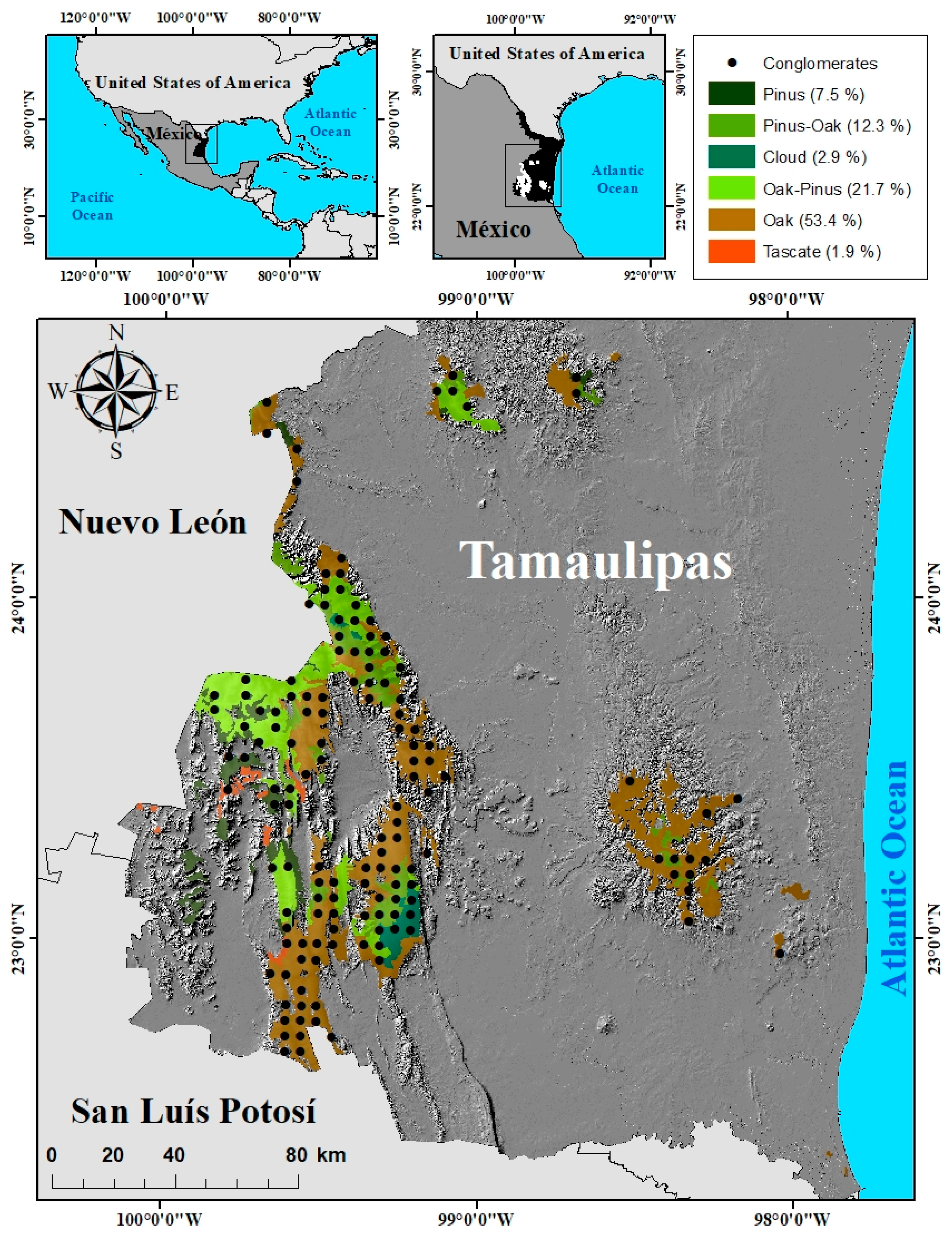
2.1. Study Area
2.2. Description of the Study Area
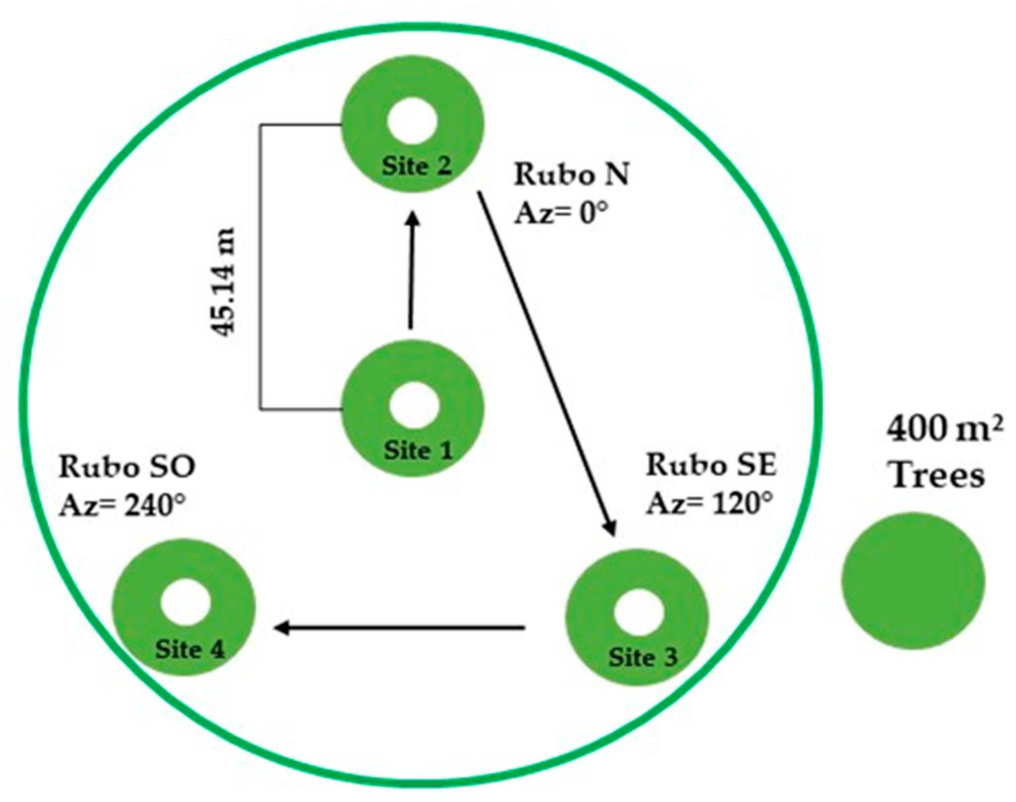
2.3. Database
2.4. Fuel Load Estimation
2.5. Fuel Load Comparison between Models
2.6. Prediction Fuel Load
2.6.1. Prediction Models
- Y = dependent variable (fuel load obtained from models)
- b = coefficient
- S = single variable
- D = double interaction of variables
- T = triple interaction of variables
- C = quadruple interaction of variables
- Q = quintuple to interaction of variables
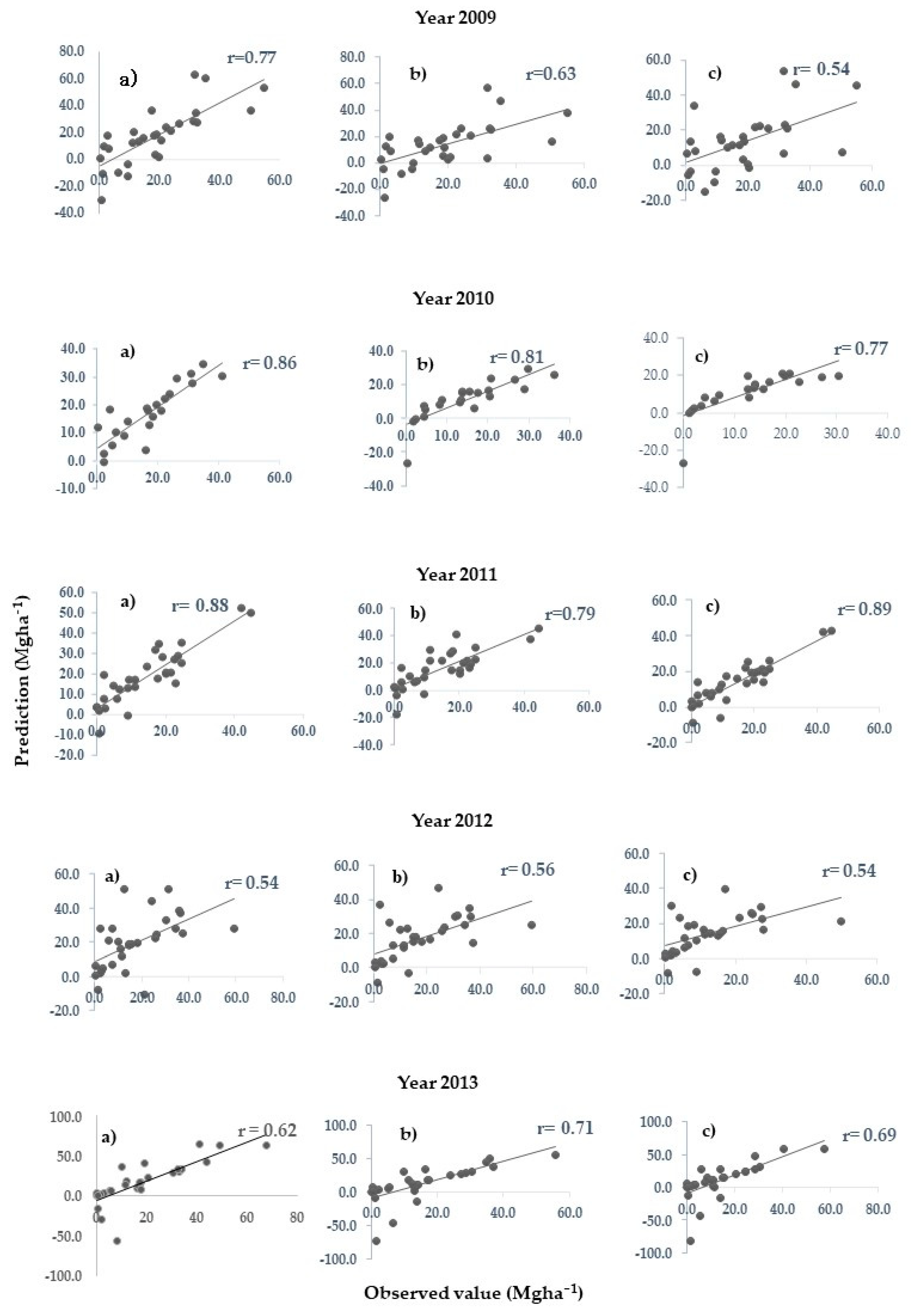
2.6.2. Model Validation
2.7. Genus and Species Contribution
2.8. Temporal Variations in Fuel Load Categories by Type of Forest
3. Results
3.1. Fuel Load
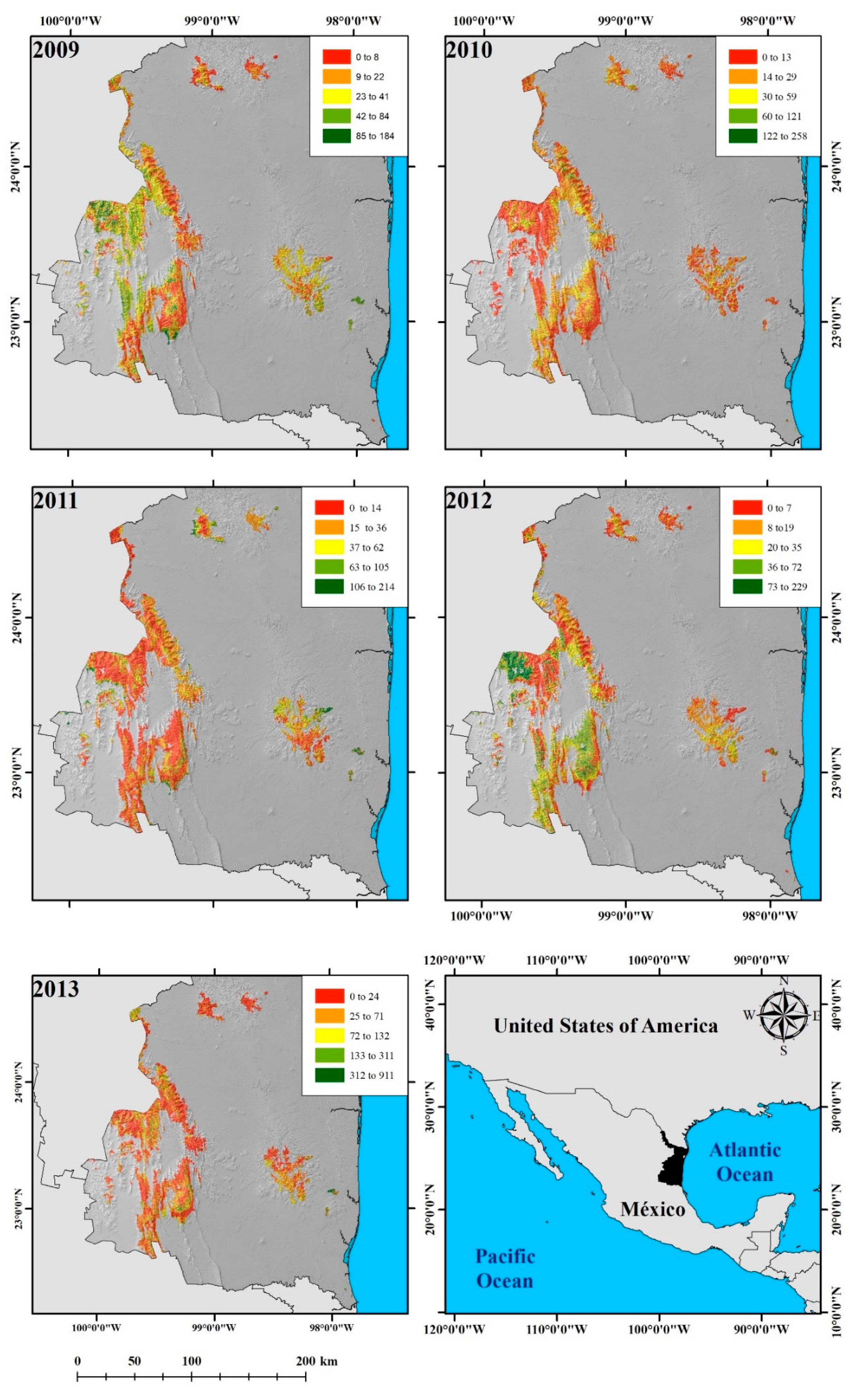
3.2. Prediction
3.3. Contribution of Genera and Species to Fuel Load
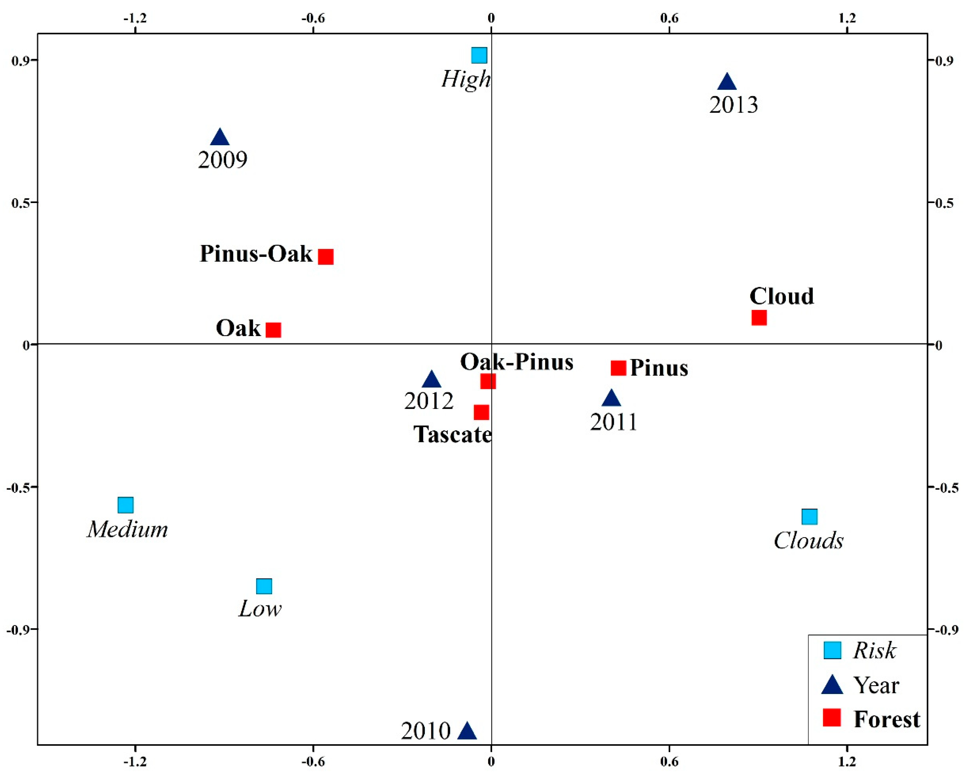
3.4. Variation in Fuel Load by Risk Forest Fires
4. Discussion
5. Conclusions
Author Contributions
Funding
Institutional Review Board Statement
Informed Consent Statement
Data Availability Statement
Acknowledgments
Conflicts of Interest
References
- Arroyo, L.A.; Pascual, L.; Manzanera, J.A. Fire models and methods to map fuel types: The role of remote sensing. For. Ecol. Manag. 2008, 256, 1239–1252. [Google Scholar] [CrossRef] [Green Version]
- Chuvieco, E.; Riño, D.; van Wastendonk, J.; Morsdof, F. Fuel loads and fuel type mapping. In Wildland Fire Danger Estimation and Mapping. The Role of Remote Sensing Data; World Scientific: Hackensack, NJ, USA, 2003; pp. 119–142. [Google Scholar]
- Etherington, T.; Curran, T. Global land-cover change-wildfires. In State of the World’s Plants; Royal Botanic Gardens, Kew: Richmond, UK, 2017; pp. 50–58. [Google Scholar]
- Brown, J.K. Handbook for Inventorying Downed Woody Material; USDA Forest Service General Technical Report INT-16; Department of Agriculture, Forest Service, Intermountain Forest and Range Experiment: Ogden, UT, USA, 1974; p. 24. [Google Scholar]
- Alanis-Morales, H.; Návar, J.; Domínguez, P. The effect of prescribed burning on surface runoff in pine forest stand of Chihuahua, Mexico. For. Ecol. Manag. 2000, 137, 199–207. [Google Scholar] [CrossRef]
- Bautista Rentería-Anima, J.; Treviño-Garza, E.; Návar-Chaidez, J.d.J.; Calderón, O.A.A. Caracterización de combustible leñosos en El Ejido Pueblo Nuevo, Durango. Rev. Chapingo. Ser. Cienc. For. Ambient. 2005, 11, 51–56. [Google Scholar]
- Picard, N.; Herry, M.; Mortier, F.; Trotta, C.; Saint-Andrés, L. Using bayesian model averaging to predict tree aboveground biomass. For. Sci. 2012, 58, 15–23. [Google Scholar]
- Magalhães, T.M. Site-specific height-diameter and stem volume equation for Lebombo-ironwood. Ann. For. Res. 2017, 60, 297–312. [Google Scholar] [CrossRef] [Green Version]
- Silva-Arredondo, F.M.; Návar-Cháidez, J.d.J. Estimación de factores de expansión de carbono en comunidades forestales templadas del norte de Durango, México. Rev. Chapingo. Ser. Cienc. For. Ambient. 2009, 15, 155–169. [Google Scholar]
- Martínez, A.L.; de los Santos, P.H.M.; Fierros, G.A.M.; Fierros, M.R.; Pérez, M.R.; Hernández, R.A.; Hernández, R.J. Factores de expansión y sistema de partición de biomasa aérea para pinus Chiapensis (Martínez) Andresen. Rev. Mex. Cien. For. 2018, 10, 107–132. [Google Scholar] [CrossRef] [Green Version]
- Flores-Garnica, J.; Omi, P.N. Mapeo de combustibles forestales para simulaciones del comportamiento especial del fuego usando estrategias de geomática. Agrociencia 2003, 37, 65–72. [Google Scholar]
- Beaudoin, A.; Bernier, P.Y.; Guindon, L.; Villemaire, P.; Guo, X.J.; Stinson, G.; Bergeron, T.; Magnussen, S.; Hall, R.J. Mapping Attributes of canada’s forests at moderate resolution through k NN and MODIS imagery. Can. J. For. Res. 2014, 44, 521–532. [Google Scholar] [CrossRef] [Green Version]
- Chen, X.; Vogelmann, J.; Rollins, M.; Ohlen, D.; Key, C.; Yang, L.; Huang, C.; Shi, H. Detecting post-fire burn severity and vegetation recovery using multitemporal remote sensing spectral indices and field-collected composite burn index data in a ponderosa pine forest. Int. J. Remote Sens. 2011, 32, 7905–7927. [Google Scholar] [CrossRef]
- Cortés, L.; Hernández, J.; Valencia, D.; Corvalán, P. Estimation of above-ground forest biomass using Landsat ETM+, Aster GDEM and Lidar. For. Res. 2014, 117, 1–7. [Google Scholar] [CrossRef] [Green Version]
- Domínguez-Cabrera, G.; Calderón, O.A.A.; Pérez, J.J.; Rodríguez-Laguna, R.; Díaz-Balderas, J.A. Biomasa aérea y factores de expansión de especies arbóreas en bosques del sur de Nuevo León. Rev. Chapingo. Ser. Cienc. For. Ambient. 2009, 15, 56–64. [Google Scholar]
- Riaño, D.; Chuvieco, E.; Salas, J.; Palacios, A.; Bastarrika, A. Generation of fuel type maps from Landsat TM images and ancillary data in mediterranean ecosystems. Can. J. For. Res. 2002, 32, 1301–1315. [Google Scholar] [CrossRef]
- Rodríguez-Laguna, R.; Jiménez-Pérez, J.; Aguirre-Calderón, O.; Jurado-Ibarra, E. Ecuaciones alométricas para estimar biomasa aérea en especies de encino y pino en Iturbide, N.L. Rev. Cien. For. México 2007, 32, 39–52. [Google Scholar]
- Escandón-Calderón, J.; Jong, B.H.J.; Ochoa-Gaona, S.; March-Mifsut, I.; Castillo, M.A. Evaluación de los métodos para la estimación de biomasa arbórea a través de datos Landsat TM en Jusnajab La Laguna, Chiapas, México: Estudio de caso. Investig. Geográficas 1999, 40, 71–84. [Google Scholar]
- D’Este, M.; Elia, M.; Giannico, V.; Spano, G.; Lafortezza, R.; Giovanni, S. Machine Learning Techniques for Fine Dead Fuel Load Estimation Using Multi-Source. Remote Sens. Data 2021, 13, 1658. [Google Scholar]
- Matsushita, B.; Yang, W.; Chen, J.; Onda, Y.; Qiu, G. Sensitivity of the enhanced vegetation index (EVI) and normalized difference vegetation index (NDVI) to topographic effects: A case study in high-density cypress forest. Sensors 2007, 7, 2636–2651. [Google Scholar] [CrossRef] [Green Version]
- Didan, K. 2015 Mod13q Modis/Terra Vegetation Indices 16-day L3 Global 250 M Sin Grid V006. Available online: https://lpdaac.usgs.gov/products/mod13q1v006/ (accessed on 19 August 2018).
- Mayorga, A.D.; Pazos, M.; Vélez, M. Uso del Índice normalizado de vegetación para la elaboración de planos de cultivo. Opuntia Brava 2019, 11, 261–265. [Google Scholar] [CrossRef]
- Linlin, L.; Kuenzer, C.; Wnag, C.; Guo, H.; Li, Q. Evaluation of three MODIS-Derived Vegetation Index time series for dryland vegetation dynamics monitoring. Remote Sens. 2019, 7, 7597. [Google Scholar] [CrossRef] [Green Version]
- Huang, X.; Liu, J.; Zhu, W.; Atzberger, C.; Liu, Q. The optimal threshold and vegetation index time series for retrieving crop phenology based on a modified dynamic threshold method. Remote Sens. 2019, 11, 2725. [Google Scholar] [CrossRef] [Green Version]
- Myoung, B.; Kim, S.H.; Nghiem, S.V.; Jia, S.; Whitney, K.; Kafatos, M.C. Estimating live fuel moisture from Modis satellite data for wildfire danger assessment in southern California USA. Remote Sens. 2018, 10, 87. [Google Scholar] [CrossRef] [Green Version]
- Reyes, P.; Burdett, E. Evolución de la cobertura forestal en los alcornocales próximos al estrecho de Gibraltar a través del índice de vegetación EVI. Ecosistemas 2019, 28, 73–80. [Google Scholar] [CrossRef]
- Roldán, P.; Poveda, G. variabilidad espacio-temporal de los índices NDVI y EVI. aplicación a cinco regiones colombianas. Meteol. Colom. 2006, 10, 47–59. [Google Scholar]
- Cheng, Y.; Zhang, C.; Zhao, X.; Gadow, K. Biomass-dominant species shape the productivity-diversity relationship in two temperate forests. Ann. For. Sci. 2018, 75, 75–95. [Google Scholar] [CrossRef] [Green Version]
- Smith, J. Encyclopedia Britannica. Available online: britannica.com/science/temperate-forest (accessed on 24 November 2020).
- Granados-Sánchez, D.; López-Ríos, F.G.; Hernández-García, M.A. Ecología y silvicultura en bosques templados. Rev. Chapingo Ser. Cienc. For. Ambient. 2007, 13, 67–83. [Google Scholar]
- Perea-Ardila, M.; Andrade-Castañeda, H.; Segura-Madrigal, M. Estimación de biomasa aérea y carbono con teledetección de bosques altos-andinos de Boyacá, Colombia. Estudio de caso: Santuario de fauna y flora Iguaque. Rev. Cart. 2021, 102, 91–123. [Google Scholar] [CrossRef]
- Felipe, F.L.; Denis, D. Variaciones espaciales y temporales de dos índices espectrales de vegetación en el jardín botánico nacional de Cuba, durante 1984–2020. Rev. Jard. Bot. Nac. 2021, 42, 119–136. [Google Scholar]
- Mundava, C.; Helmholz, P.; Antonius, G.T.S.; Corner, R.; McAtee, B.; Lamb, D.W. Evaluation of vegetation indices for rangeland biomass estimation in the kimberley area of western Australia. ISPRS Ann. Photogramm. Remote Sens. Spat. Inf. Sci. Tomo II 2014, 7, 47–53. [Google Scholar] [CrossRef] [Green Version]
- Dixon, D.; Callow, J.J.N.; Duncan, J.M.A.; Samantha, A. Setterfield, and Natasha Pauli. Regional-Scale Fire Severity Mapping of Eucalyptus Forests with the Landsat Archive. Remote Sens. Environ. 2022, 270, 112863. [Google Scholar] [CrossRef]
- Reyes-Cárdenas, O.; Treviño-Garza, E.; Jiménez-Pérez, J.; Aguirre-Calderón, O.A.; Cuéllar-Rodríguez, L.; Flores-Garnica, J.; Cárdenas-Tristán, A. Modelización de biomasa forestal aérea mediante técnicas determinísticas y estocásticas. Madera y Bosques 2019, 25, e2511622. [Google Scholar] [CrossRef]
- Santillán, M.L. Los Hotspots de Biodiversidad, Regiones Insustituibles en el Planeta. 2021. Available online: https://ciencia.unam.mx/leer/1060/los-hotspot-de-biodiversidad-regiones-insustituibles-en-el-planeta#:~:text=Los%20tres%20hotspots%20que%20se,pino%2Dencino%2C%20que%20incluye%20las (accessed on 27 November 2021).
- Ecosystem, C. Madreand Pine-Oak Woodlands-Sources. 2021. Available online: https://www.cepf.net/our-work/biodiversity-hotspots/madrean-pine-oak-woodlands/threats (accessed on 28 November 2021).
- Santini, N.; Adame, F.; Nolan, R.; Miquelajauregui, Y.; Piñero, D.; Mastretta-Yanes, A.; Cuervo-Robayo, A.; Eamus, D. Storage of organic carbon in the soils of mexican temperate forests. For. Ecol. Manag. 2019, 446, 115–125. [Google Scholar] [CrossRef]
- Comisión Nacional para el Conocimiento y Uso de la Biodiversidad. Bosques Templados. 2019. Available online: https://www.biodiversidad.gob.mx/ecosistemas/bosqueTemplado (accessed on 11 October 2021).
- Comisión Nacional Forestal. Reporte final de Incendios Forestales. 2019. Available online: https://www.gob.mx/cms/uploads/attachment/file/522446/Cierre_de_la_Temporada_2019.pdf (accessed on 28 October 2020).
- Rzedowski, J. La vegetación de México. In Comisión Nacional Para El Conocimiento Y Uso de la Biodiversidad, México, 1st ed.; Digital México: Ciudad de México, México, 2006; p. 504. [Google Scholar]
- Secretaría de Medio Ambiente y Recursos Naturales. Anuario Estadístico de la Producción Nacional Forestal; Dirección de Gestión Forestal y de Suelo: Ciudad de México, México, 2012. [Google Scholar]
- National Institute of Statistics and Geography. Conjunto de Datos Vectoriales de Uso de Suelo Y Vegetación; Escala 1:250000, Serie VI; Instituto Nacional de Estadística y Geografía: Aguascalientes, México, 2016. [Google Scholar]
- Secretaría de Medio Ambiente y Recursos Naturales. Comisión Nacional Forestal. Inventario Estatal Forestal Y de Suelos-Tamaulipas 2014; SEMARNAT, CONAFOR: Zapopan, México, 2015; p. 183. [Google Scholar]
- Rojas-García, F.; de Jong, B.H.J.; Martínez-Zurimendí, P.; Paz-Pellat, F. Database of 478 allometric equations to estimate biomass for mexican trees and forests. Ann. For. Sci. 2015, 72, 835–864. [Google Scholar] [CrossRef] [Green Version]
- Soriano-Luna, M.d.l.A.; Angeles-Pérez, G.; Martínez-Trinidad, T.; Plascencia-Escalante, F.O.; Razo-Zárate, R. Estimación de biomasa aérea por componente estructural en zacualtipán, Hidalgo, México. Agrociencia 2015, 49, 423–438. [Google Scholar]
- Brown, S.; Schoeder, P.; Birdsey, R. Aboveground biomass distribution of us eastern hardwood forests and the Use of large trees as an indicator of forest development. For. Ecol. Manag. 1997, 96, 37–47. [Google Scholar] [CrossRef]
- Sokal, R.R.; Rohlf, F.J. Biometry: The Principples and Practice of Statistics, 3rd ed.; Biological Research; Freeman: New York, NY, USA, 2005. [Google Scholar]
- Reyes-Díez, A.; Alcaraz-Segura, D.; Cabello-Piñar, J. Implicaciones del filtrado de calidad del índice de vegetación EVI para el seguimiento funcional de ecosistemas. Rev. De Teledetección 2015, 43, 11–29. [Google Scholar] [CrossRef] [Green Version]
- Mas, J.F. Aplicación Del Sensor Modis Para El Monitoreo del Territorio; SEMARNAT: Ciudad de México, México, 2011. [Google Scholar]
- Phillips, S.J.; Anderson, R.P.; Schapire, R.E. Maximum entropy modeling of species geographic distributions. Ecol. Model. 2006, 190, 231–259. [Google Scholar] [CrossRef] [Green Version]
- Shiker, M. Multivariate Statistical Analysis. Jur. Sci. 2012, 6, 55–66. [Google Scholar]
- Wold, S.; Sjöström, S.; Eriksson, L. Pls-regression: A basic tool of chemometrics. Chemom. Intell. Lab. Syst. 2001, 58, 109–130. [Google Scholar] [CrossRef]
- Wold, S. Cross-validatory estimation of the number of components in factor and principal components models. Technometrics 1978, 20, 405. [Google Scholar] [CrossRef]
- Rubio Hurtado, M.J.; Silvente, V.B. Cómo aplicar las pruebas pramétricas bivariadas t de student y anova en spss. Caso práctico. REIRE Rev. D’innovación I Recer. En Educ. 2012, 5, 83–100. [Google Scholar]
- Hammer, O.; Harper, D.A.T.; Ryan, D. Paleontological statistics software package for education and data analysis. Palaentologia Electonica 2001, 4, 9. [Google Scholar]
- Scott, J.H.; Burgan, R.E. Standard Fire Behavior Fuel Models: A Comprehesive Set for Use with Rothermel’S Surface Fire Spread Model; General Technical Report RMRS-GTR-153; US Department of Agriculture, Forest Service, Rocky Mountain Research Station: Fort Collins, CO, USA, 2005.
- Anderson, M.J. A new method for non-parametric multivariate analysis of variance. Austral Ecol. 2001, 26, 39–90. [Google Scholar]
- Bray, J.R.; Curtis, J.T. An ordination of the upland forest communities of southern Wisconsin. Ecol. Monogr. 1957, 27, 325–349. [Google Scholar] [CrossRef]
- Clarke, K.R. Non-parametric multivariate analyses of change in community structure. Austral. Ecol. 1993, 18, 117–143. [Google Scholar] [CrossRef]
- Legendre, P. Spatial autocorrelation: Trouble or new paradigm? Ecology 2003, 74, 1659–1673. [Google Scholar] [CrossRef]
- Stratoulias, D.; Nuthammachot, N.; Suepa, T.; Phoungthong, K. Assessing the spectral information of Sentinel-1 and Sentinel-2 Satellites for above-ground biomass retrieval of a tropical forest. ISPRS Int. J. Geo-Inf. 2022, 11, 199. [Google Scholar] [CrossRef]
- Nuthammachot, N.; Askar, A.; Stratoulias, D.; Wicaksono, P. Combined use of Sentinel-1 and Sentinel-2 Data for improving above-ground biomass estimation. Geocarto Int. 2022, 37, 366–376. [Google Scholar] [CrossRef]
- Campbell, M.J.; Dennison, P.E.; Kerr, K.L.; Brewer, S.C.; Anderegg, W.R.L. Scaled biomass estimation in woodland ecosystems: Testing the individual and combined capacities of satellite multispectral and Lidar Data. Remote Sens. Environ. 2021, 262, 112511. [Google Scholar] [CrossRef]
- Huang, H.; Liu, C.; Wang, X.; Zhou, X.; Gong, P. Integration of multi-resource remotely sensed data and allometric models for forest aboveground biomass estimation in China. Remote Sens. Environ. 2019, 221, 225–234. [Google Scholar] [CrossRef]
- Ehlers, D.; Wang, C.; Coulston, J.; Zhang, Y.; Pavelsky, T.; Frankenberg, E.; Woodcock, C.; Song, C. Mapping forest aboveground biomass using multisource remotely sensed data. Remote Sens. 2022, 14, 1115. [Google Scholar] [CrossRef]
- Cabello, J.; Alcaraz-Segura, D.; Ferrero, R.; Liras, E. The role of vegetation and lithology in the spatial and inter-annual response of EVI to climate in drylands of southeastern Spain. J. Arid. Environ. 2012, 79, 76–83. [Google Scholar] [CrossRef]
- Kong, B.; Huan, Y.; Rongxiang, D.; Wang, Q. Quantitative estimation of biomass of alpine grasslands using hyperspectral remote sensing. Ran. Ecol. Manag. 2018, 72, 336–346. [Google Scholar] [CrossRef]
- Casiano, M.; Paz, F. Caracterización fenológica de bosques tropicales caducifolios usando información espectral: Experimentos con componentes. Terra Lat. 2014, 32, 259–271. [Google Scholar]
- Testa, S.; Soundaani, K.; Boschetti, L.; Borgogno, M.E. MODIS-derived EVI; NDVI and WDRVI time series to estimate phenological metric in French deciduous forests. Int. J. Appl. Earth Obs. Geoinf. 2018, 64, 132–144. [Google Scholar] [CrossRef]
- Pflugmacher, D.; Cohen, W.B.; Kennedy, R.E.; Yang, Z. Using Landsat-derived disturbance and recovery history and lidar to map forest biomass dynamics. Remote Sens. Environ. 2013, 151, 124–137. [Google Scholar] [CrossRef]
- Zhang, G.; Ganguly, S.; Nemani, R.; White, M.; Milesi, C.; Hashimoto, H.; Wang, W.; Saatchi, S.; Yu, Y.; Myneni, R. Estimation of forest aboveground biomass in California using canopy height and leaf area index estimated from satellite data. Remote Sens. Environ. 2014, 151, 44–56. [Google Scholar] [CrossRef]
- García, M.; Saatchi, S.; Casas, A.; Koltunov, A.; Ustin, S.; Ramírez, C.; Gutierrez, G.; Balzter, H. Quantifying biomass consumpion and carbon release from the California rim fire by integrating airborne Lidar and Landsat OLI data. J. Geophys. Ress. Solid Earth 2017, 122, 340–353. [Google Scholar] [CrossRef]
- Duguy, B.; Alloza, J.A.; Baeza, M.J.; de la Riva, J.; Echeverría, M.; Ibarra, P.; Llovet, J.; Cabello, F.P.; Rovira, P.; Vallejo, R.V. Modelling the ecological vulnerability to forest fire in mediterranean ecosystems using geographic information technologies. Environ. Manag. 2012, 50, 1012–1026. [Google Scholar] [CrossRef]
- Tonbul, H.; Kavzoglu, T.; Kaya, S. Assessment of fire severity and post-fire regeneration based on topographical features using multitemporal Landsat imagery: A case study in Mersin, Turkey. Remote Sens. Spat. Inf. Sci. 2016, XLI-B8, 763–769. [Google Scholar] [CrossRef]
- García, M.; Saatchi, S.; Casas, A.; Koltunov, A.; Ustin, S.; Ramirez, C.; Balzter, H. Extrapolating forest canopy fuel properties in the California rim fire by combining airborne Lidar and Landsat Oli data. Remore Sens. 2017, 9, 394. [Google Scholar] [CrossRef] [Green Version]
- Torres, P.T.F.; Romeiro, N.M.J.; Santos, A.C.A.; Neto, O.R.R.; Lima, S.G.; Zanuncio, J.C. Fire danger index efficiency as a function of fuel moinsture and fire behavoir. Sci. Total Environ. 2018, 1, 1304–1310. [Google Scholar] [CrossRef] [PubMed]
- Comisión Nacional Forestal. Guía Práctica Para Comunicadores; Comisión Nacional Forestal: Zapopan, México, 2010; p. 54. [Google Scholar]
- Chuvieco, E. Fundamentos de Teledetección Espacial, 2nd ed.; RIALP: Madrid, Spain, 2000; p. 224. [Google Scholar]
- Duff, T.; Bell, T.; York, A. Predicting continuous variation in forest fuel load using biophysical models: A case study in south-eastern Australia. Int. J. Wildland Fire 2012, 22, 318–332. [Google Scholar] [CrossRef]
- Vega-García, D.; Tatay, J.; Blanco, R.; Chuvieco, E. Evaluation of the influence of local fuel homogeneity on fire hazard through Landsat-5 Tm texture measures. Photogramm. Eng. Remote Sens. 2010, 76, 853–864. [Google Scholar] [CrossRef]
- Fares, S.; Bajocco, S.; Salvati, L.; Camarretta, N.; Dupuy, J.; Xanthopoulos, G.; Guijarro, M.; Madrigal, J.; Hernando, C.; Corona, P. Characterizing potential wildland fire fuel in live vegetation in the Mediterranean region. Ann. For. Sci. 2017, 74, 1. [Google Scholar] [CrossRef] [Green Version]
- Vega-Nieva, D.J.; Briseño-Reyes, J.; Nava-Miranda, M.G.; Calleros-Flores, E.; López-Serrano, P.M.; Corral-Rivas, J.J.; Montiel-Antuna, E.; Cruz-López, M.I.; Cuahutle, M.; Ressl, R.; et al. Developing models to predict the number of fire hotspots from an accumulated fuel dryness index by vegetation type and region in México. Forests 2018, 9, 190. [Google Scholar] [CrossRef] [Green Version]
- Comisión Nacional para el Conocimiento y Uso de la Biodiversidad. Sistema de alerta Temprana de Incendios. México. 2018. Available online: www.incendios.conabio.gob.mx (accessed on 29 March 2022).
- Government of Natural Resources Canada. 2021. Available online: https://cwfis.cfs.nrcan.gc.ca/background/summary/fdr (accessed on 2 January 2022).
- Matt, W.J.; Larry, B. National Fire Danger Rating System. Available online: https://www.firelab.org/project/national-fire-danger-rating-system (accessed on 21 November 2021).
- Xelhuantzi, C.J.; Flores, G.J.G.; Chavez, D.A.A. Análisis comparativo de carga de combustible en ecosistemas forestales afectados por incendios. Rev. Mex. Cien. For. 2011, 2, 37–52. [Google Scholar]
- Pontes-Lopes, A.; Dalagnol, R.; Dutra, A.C.; Silva, C.V.d.; Graça, P.M.L.d.; de Aragão, L.E.d.e.C. Quantifying post-fire changes in the aboveground biomass of an Amazonian forest based on field and remote sensing data. Remote Sens. 2022, 14, 1545. [Google Scholar] [CrossRef]
- Pérez Mojica, E.; Valencia-A, S. Estudio preliminar del género Quercus (Fagacea) en Tamaulipas, México. Acta Botánica Mex. 2017, 120, 59–111. [Google Scholar] [CrossRef]
- Cavender-Bares, J. Diversification, adaptation; community assembly of the american Oaks (Quercus), a model clade for integrating ecology and evolution. New Phytol. 2019, 221, 669–692. [Google Scholar] [CrossRef] [Green Version]
- Thyroff, E.; Burney, O.; Mickelbart, M.; Jacobs, D. Unraveling shade tolerance and plasticity of semi-evergreen oaks: Insights from maritime forest live Oak restoration. Front. Plant Sci. 2019, 10, 1526. [Google Scholar] [CrossRef] [Green Version]
- Rothaermel, R.C. A mathematical model for predicting fire spread in wildland fuels. In Intermountain Forest and Range Experiments; US Department of Agriculture, Forest Service, Intermountain Forest and Range Experiment Station: Ogden, UT, USA, 1972. [Google Scholar]
- Balb, E.; Alexander, H.D.; Siegert, C.M.; Willis, J.M. Could canopy, bark; leaf litter traits of encroaching non-oak species influence future flammability of upland oak forest. For. Ecol. Manag. 2019, 458, 117731. [Google Scholar] [CrossRef]


| Model | Species | Equation | Source |
|---|---|---|---|
| Model real stock | Temperate forest | Vt = α × DB1 × HB2 | Silva-Arredondo y Návar-Cháidez, (2009) |
| Model aboveground biomass | Quercus cambyi | B = α − 2.3112 × D2.4497 | Rodríguez-Laguna et al. (2007) |
| Quercus laceyi | B = α − 2.4344 × D2.5069 | Rodríguez-Laguna et al. (2007) | |
| Quercus rysophylla | B = α − 2.2089 × D2.3736 | Rodríguez-Laguna et al. (2007) | |
| Quercus rugosa | B = 0.089 × DN2.5226 | Rojas-García et al. (2015) | |
| Quercus ssp | B = 0.45534 × DN2 | Rojas-García et al. (2015) | |
| Pinus greggi | B = −0.177 + (0.015 × DN2) × h) | Rojas-García et al. (2015) | |
| Pinus moctezumae | B= 1.30454 × DN2.3644444 | Rojas-García et al. (2015) | |
| Pinus nelsonni | B = 0.1229 × DN2.3964 | Rojas-García et al. (2015) | |
| Pinus teocote | B = 0.032495 × DN2.766578 | Rojas-García et al. (2015) | |
| Juniperus flaccida | B = α − 1.6469 × DN2.1255 | Rodríguez-Luna et al. (2007) | |
| Broadleaf forest | B = EXP(−B0) × (DN2 ∗ h) B1 | Soriano-Luna et al. (2015) | |
| Model coniferous species | Coniferous forest | B = 5.0 + 150000 × DN − 2.7/DN − 2.7 + 364946 | Brown et al. (1997) |
| Variable | Source | Accessed Date |
|---|---|---|
| Vegetation height (m) | http://www.earthenv.org | 5 April 2020 |
| Evapotranspiration | https://worldclim.org | |
| EVI | https://earthexplorer.usgs.gov | |
| Elevation (msnm) | https://www.inegi.org.mx | |
| Slope % | https://www.inegi.org.mx | |
| Annual precipitation (mm) | https://worldclim.org | |
| Annual average temperature (°C) | https://worldclim.org |
| Year | Model | s | Dif | t Value | d.f | P | |
|---|---|---|---|---|---|---|---|
| 2009 | Real stock | 17.1 | 21.3 | 3.7 | 0.7 | 28.0 | 0.483 |
| Aboveground biomass | 13.4 | 16.7 | |||||
| Real stock | 17.1 | 21.3 | 3.6 | 0.7 | 28.0 | 0.458 | |
| Coniferous species | 13.4 | 16.4 | |||||
| Aboveground biomass | 13.4 | 16.7 | 0.0 | 0.0 | 28.0 | 0.981 | |
| Coniferous species | 13.4 | 16.4 | |||||
| 2010 | Real stock | 17.1 | 9.9 | 6.1 | 1.7 | 21.0 | 0.097 |
| Aboveground biomass | 10.9 | 11.9 | |||||
| Real stock | 17.1 | 9.9 | 6.5 | 2.4 | 21.0 | 0.024 | |
| Coniferous species | 10.6 | 10.8 | |||||
| Aboveground biomass | 10.9 | 11.9 | 0.4 | 0.1 | 21.0 | 0.915 | |
| Coniferous species | 10.6 | 10.8 | |||||
| 2011 | Real stock | 18.4 | 14.1 | 2.7 | 0.977 | 29.0 | 0.336 |
| Aboveground biomass | 15.7 | 14.1 | |||||
| Real stock | 18.4 | 14.1 | 4.7 | 6.9 | 29.0 | 0.000 | |
| Coniferous species | 13.65 | 11.8 | |||||
| Aboveground biomass | 15.7 | 14.1 | 2.0 | 0.7 | 29.0 | 0.432 | |
| Coniferous species | 13.7 | 11.9 | |||||
| 2012 | Real stock | 19.3 | 15.9 | 2.5 | 1.5 | 30.0 | 0.129 |
| Aboveground biomass | 16.7 | 12.9 | |||||
| Real stock | 19.3 | 15.9 | 5.5 | 3.2 | 30.0 | 0.029 | |
| Coniferous species | 13.8 | 11.1 | |||||
| Aboveground biomass | 16.7 | 12.9 | 3.0 | 5.9 | 30.0 | 0.000 | |
| Coniferous species | 13.8 | 11.1 | |||||
| 2013 | Real stock | 16.7 | 26.2 | 5.4 | 0.8 | 28.0 | 0.427 |
| Aboveground biomass | 11.3 | 26.4 | |||||
| Real stock | 16.7 | 26.2 | 7.0 | 1.1 | 28.0 | 0.278 | |
| Coniferous species | 9.7 | 27.3 | |||||
| Aboveground biomass | 11.3 | 26.4 | 1.6 | 0.2 | 28.0 | 0.833 | |
| Coniferous species | 9.7 | 27.3 |
| Year | Model | Data | s | Dif. | t Value | d.f | P | |
|---|---|---|---|---|---|---|---|---|
| 2009 | Real stock | Observed | 20.27 | 17.00 | 3.14 | 0.45 | 7 | 0.67 |
| Predicted | 17.13 | 30.27 | ||||||
| Aboveground biomass | Observed | 20.27 | 17.00 | 11.15 | 1.63 | 7 | 0.15 | |
| Predicted | 9.12 | 23.99 | ||||||
| Coniferous species | Observed | 20.27 | 17.00 | 10.30 | 1.56 | 7 | 0.16 | |
| Predicted | 9.97 | 19.27 | ||||||
| 2010 | Real stock | Observed | 20.21 | 7.90 | 2.37 | 1.55 | 8 | 0.16 |
| Predicted | 17.83 | 8.69 | ||||||
| Aboveground biomass | Observed | 17.26 | 7.66 | 2.44 | 1.83 | 8 | 0.11 | |
| Predicted | 14.82 | 7.71 | ||||||
| Coniferous species | Observed | 15.18 | 5.56 | 1.13 | 1.08 | 8 | 0.31 | |
| Predicted | 14.06 | 4.50 | ||||||
| 2011 | Real stock | Observed | 17.70 | 13.63 | −11.31 | −5.90 | 6 | 0.001 |
| Predicted | 29.01 | 13.80 | ||||||
| Aboveground biomass | Observed | 18.31 | 13.70 | −5.66 | −1.48 | 6 | 0.19 | |
| Predicted | 23.97 | 12.45 | ||||||
| Coniferous species | Observed | 18.31 | 13.70 | −2.49 | −1.20 | 6 | 0.27 | |
| Predicted | 20.80 | 11.02 | ||||||
| 2012 | Real stock | Observed | 17.89 | 11.01 | −8.93 | −1.15 | 7 | 0.29 |
| Predicted | 26.82 | 19.68 | ||||||
| Aboveground biomass | Observed | 17.89 | 11.01 | −4.43 | −0.92 | 7 | 0.39 | |
| Predicted | 22.32 | 8.25 | ||||||
| Coniferous species | Observed | 13.03 | 8.35 | −5.88 | −1.62 | 7 | 0.15 | |
| Predicted | 18.91 | 6.12 | ||||||
| 2013 | Real stock | Observed | 13.07 | 17.01 | −1.13 | −0.26 | 6 | 0.81 |
| Predicted | 14.20 | 26.45 | ||||||
| Aboveground biomass | Observed | 11.60 | 14.81 | −0.65 | −0.24 | 6 | 0.82 | |
| Predicted | 12.24 | 20.31 | ||||||
| Coniferous species | Observed | 9.57 | 12.98 | −0.86 | −0.24 | 6 | 0.82 | |
| Predicted | 10.43 | 20.42 |
| Genus | Contribution (%) | Acumulative Contribution (%) | Risk Forest Fire | ||
|---|---|---|---|---|---|
| High | Medium | Low | |||
| Quercus | 68.7 | 68.7 | 66.7 | 57.2 | 31.1 |
| Pinus | 17 | 85.7 | 11.9 | 2.8 | 3.1 |
| Arbutus | 6.2 | 91.9 | 3.6 | 3.1 | 1.8 |
| Juniperus | 3.5 | 95.4 | 3.8 | 2 | 0.6 |
| Liquidambar | 2.6 | 98 | 1.7 | 0.9 | 0.1 |
| Cedrela | 0.5 | 98.5 | 0.2 | 0.1 | 0.1 |
| Carpinus | 0.5 | 99.1 | 0.3 | 0 | 0.1 |
| Cupressus | 0.4 | 99.4 | 0.1 | 0 | 0.1 |
| Conestegia | 0.2 | 99.7 | 0.1 | 0 | 0 |
| Cercocarpus | 0.2 | 99.9 | 0 | 0 | 0.2 |
| Randia | 0.1 | 100 | 0 | 0 | 0.1 |
| Sargentia | 0 | 100 | 0 | 0 | 0 |
Publisher’s Note: MDPI stays neutral with regard to jurisdictional claims in published maps and institutional affiliations. |
© 2022 by the authors. Licensee MDPI, Basel, Switzerland. This article is an open access article distributed under the terms and conditions of the Creative Commons Attribution (CC BY) license (https://creativecommons.org/licenses/by/4.0/).
Share and Cite
Aradillas-González, M.d.R.; Vargas-Tristán, V.; Azuara-Domínguez, A.; Horta-Vega, J.V.; Manjarrez, J.; Rodríguez-Castro, J.H.; Venegas-Barrera, C.S. Spatial and Temporal Variations of Predicting Fuel Load in Temperate Forests of Northeastern Mexico. Forests 2022, 13, 988. https://doi.org/10.3390/f13070988
Aradillas-González MdR, Vargas-Tristán V, Azuara-Domínguez A, Horta-Vega JV, Manjarrez J, Rodríguez-Castro JH, Venegas-Barrera CS. Spatial and Temporal Variations of Predicting Fuel Load in Temperate Forests of Northeastern Mexico. Forests. 2022; 13(7):988. https://doi.org/10.3390/f13070988
Chicago/Turabian StyleAradillas-González, Ma. del Rosario, Virginia Vargas-Tristán, Ausencio Azuara-Domínguez, Jorge Víctor Horta-Vega, Javier Manjarrez, Jorge Homero Rodríguez-Castro, and Crystian Sadiel Venegas-Barrera. 2022. "Spatial and Temporal Variations of Predicting Fuel Load in Temperate Forests of Northeastern Mexico" Forests 13, no. 7: 988. https://doi.org/10.3390/f13070988