
Crown Structure Metrics to Generalize Aboveground Biomass Estimation Model Using Airborne Laser Scanning Data in National Park of Hainan Tropical Rainforest, China

 and
and 
Abstract
:1. Introduction
2. Materials and Methods
2.1. Materials
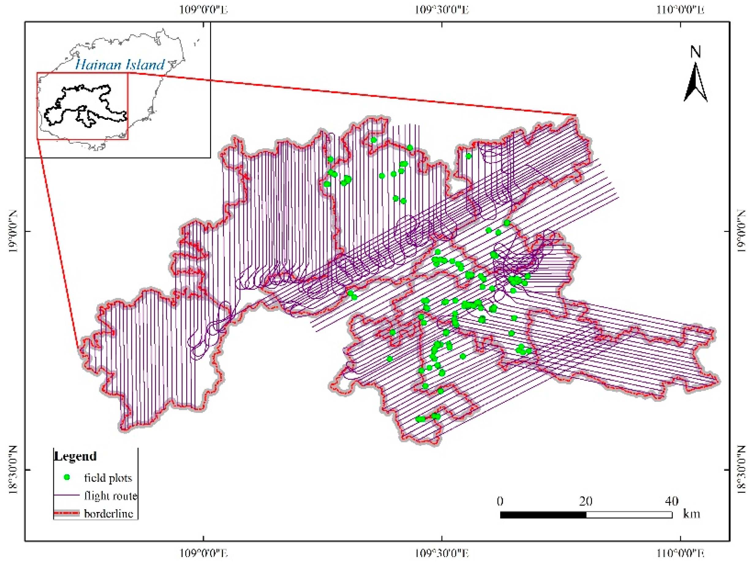
2.1.1. Study Area
2.1.2. ALS Data Acquisition
2.1.3. ALS Data Processing
2.1.4. Inventory Data
2.2. Methods
2.2.1. AGB Calculation
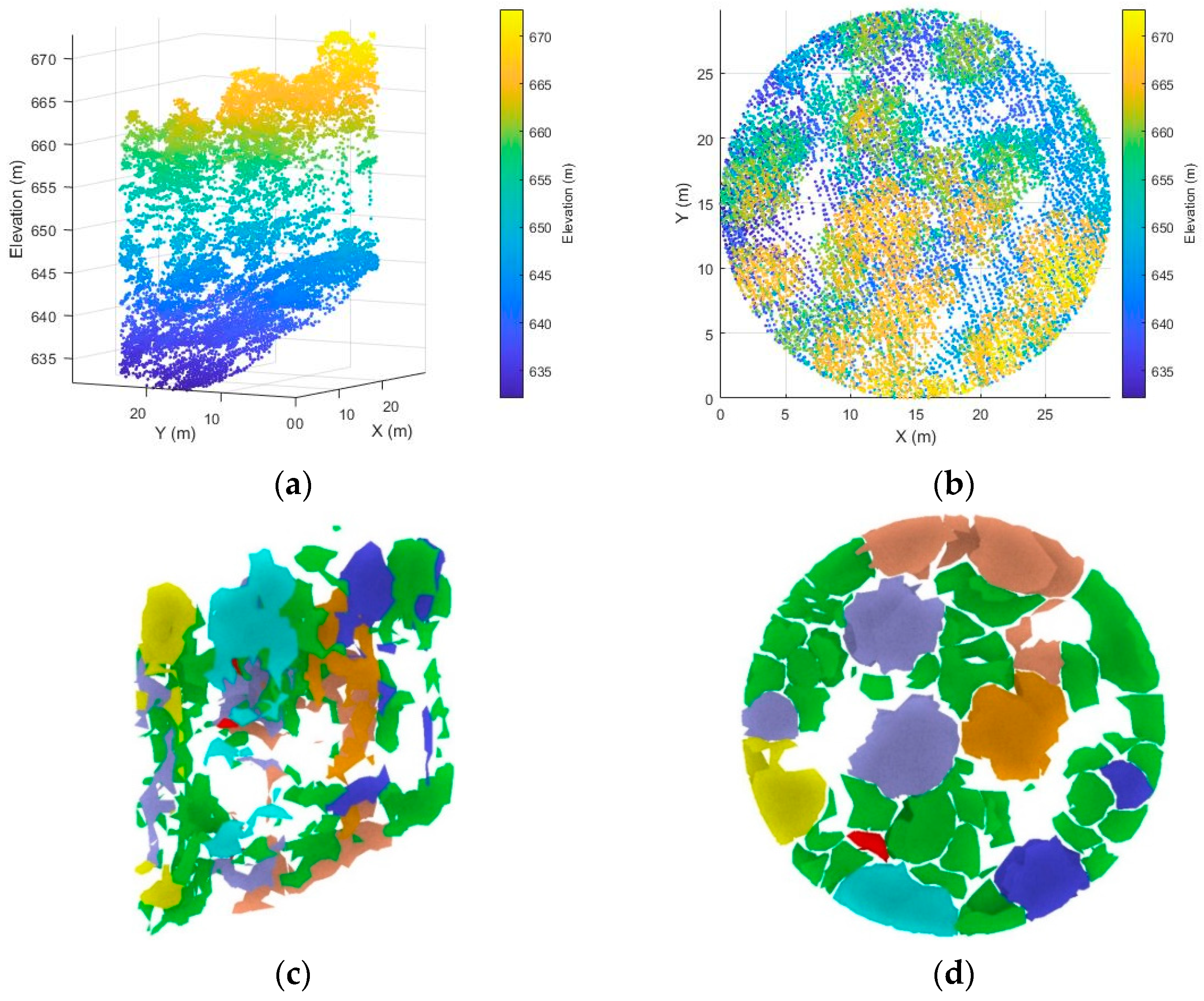
2.2.2. Crown Features Extraction
2.2.3. Feature Variables Extraction
- (a)
- Height metrics
- (b)
- Intensity metrics
- (c)
- Alpha-shape metrics
- (d)
- Stand metrics
2.2.4. Regression Modeling of AGB
2.2.5. Precision Assessment
3. Results
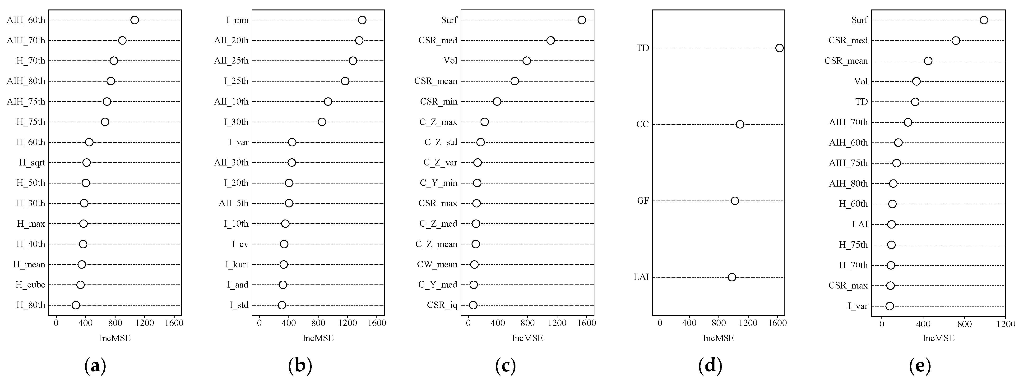
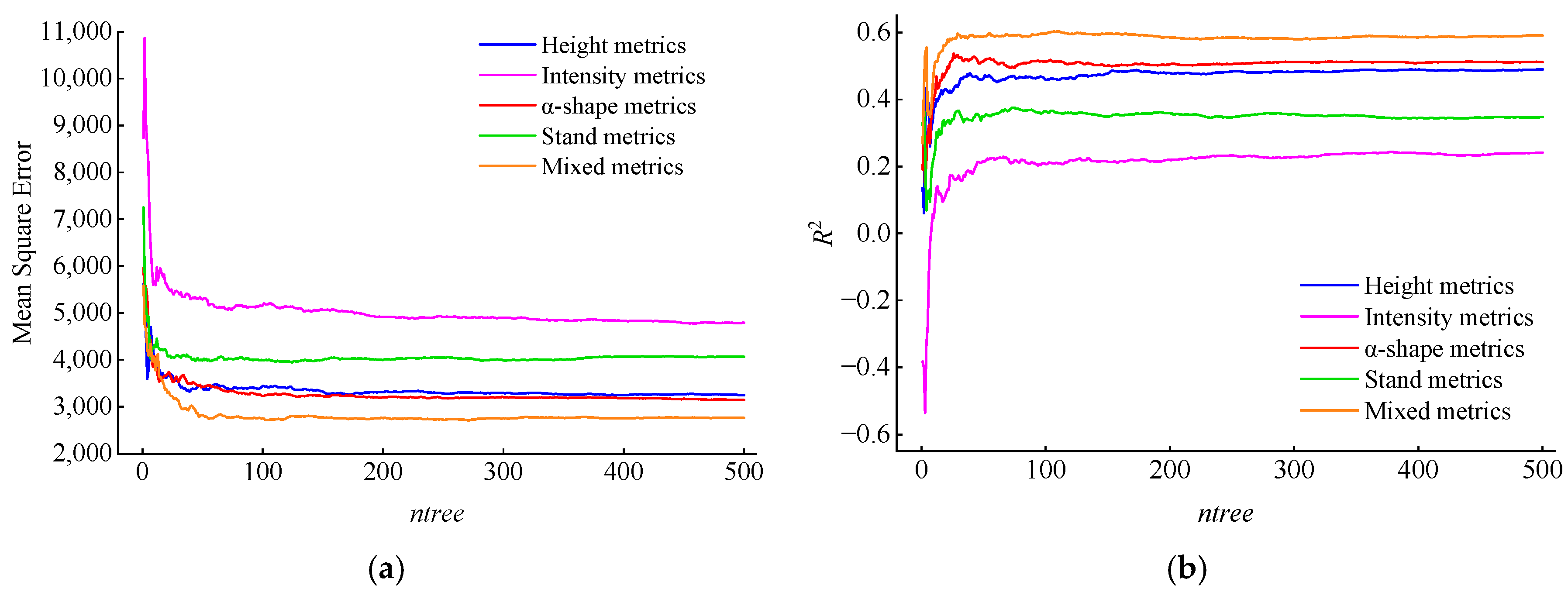
3.1. Feature Selection
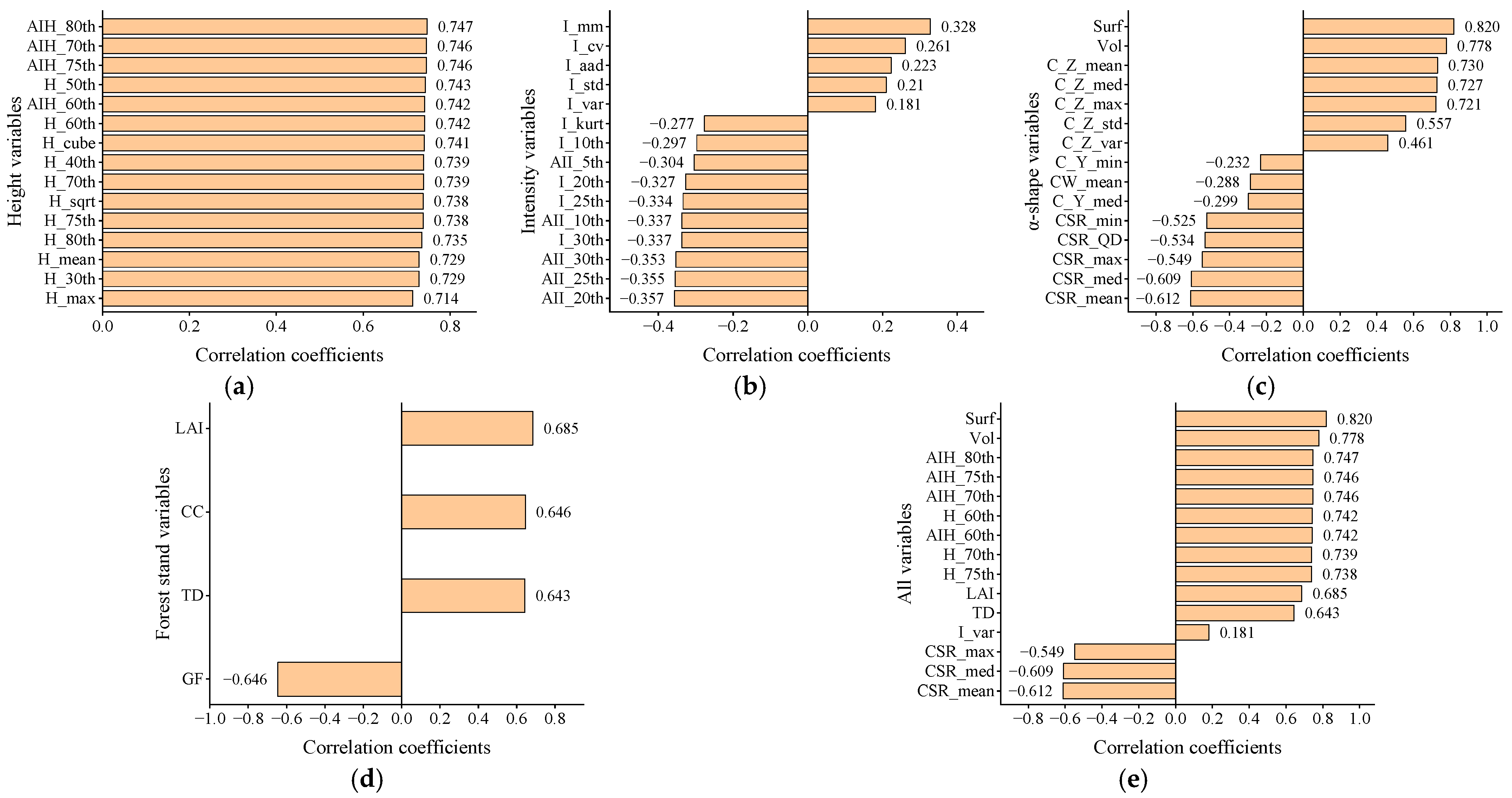
3.2. Correlation Analysis
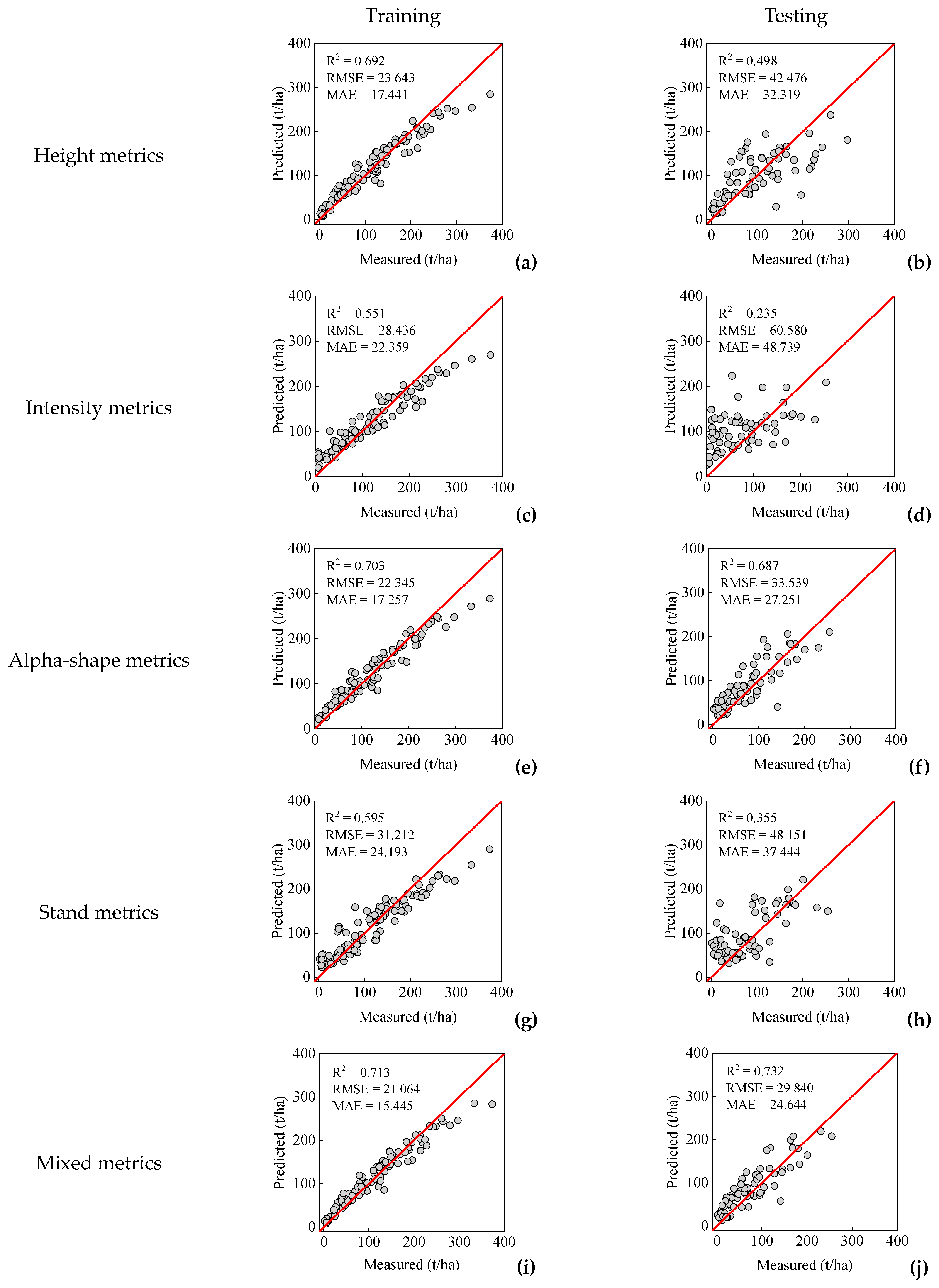
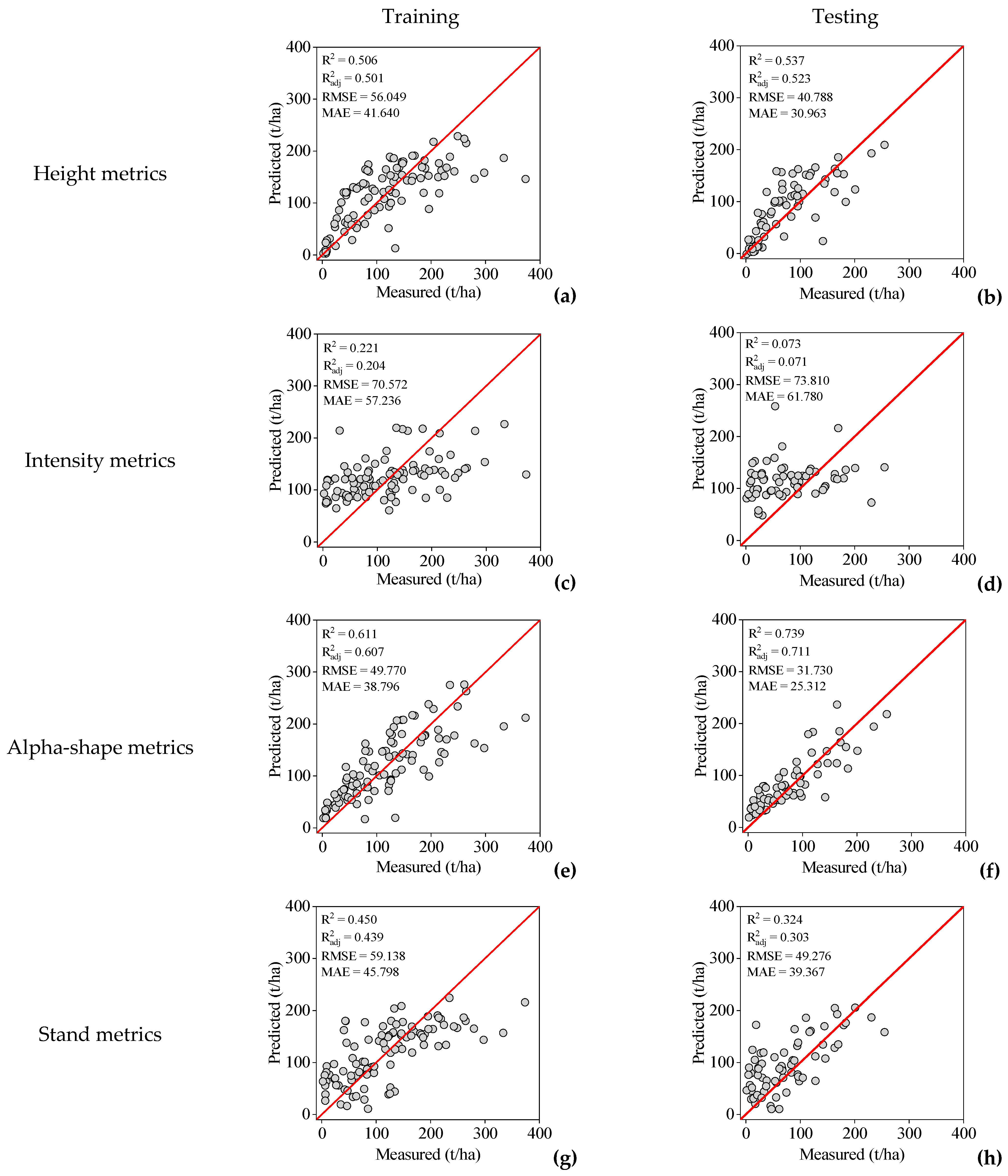
3.3. AGB Estimation Models
3.4. Regression Model Precision Assessment
4. Discussion
4.1. The Important Roles of Variables from ALS for AGB Estimation at Stand Level
4.2. Effects on Structure of Individual Trees Based on Alpha-Shape Analysis
4.3. Regression Models of AGB Estimation
4.4. Other Factors for Characterizing AGB Estimation
5. Conclusions
Author Contributions
Funding
Data Availability Statement
Acknowledgments
Conflicts of Interest
References
- West, P.W. Tree and Forest Measurement; Springer International Publishing: Cham, Switzerland, 2015; ISBN 978-3-319-14707-9. [Google Scholar]
- Wang, Q.; Pang, Y.; Chen, D.; Liang, X.; Lu, J. Lidar Biomass Index: A Novel Solution for Tree-Level Biomass Estimation Using 3D Crown Information. For. Ecol. Manag. 2021, 499, 119542. [Google Scholar] [CrossRef]
- Iida, S.; Shimizu, T.; Tamai, K.; Kabeya, N.; Shimizu, A.; Ito, E.; Ohnuki, Y.; Chann, S.; Levia, D.F. Evapotranspiration from the Understory of a Tropical Dry Deciduous Forest in Cambodia. Agric. For. Meteorol. 2020, 295, 108170. [Google Scholar] [CrossRef]
- Almeida, D.R.A.; Almeyda Zambrano, A.M.; Broadbent, E.N.; Wendt, A.L.; Foster, P.; Wilkinson, B.E.; Salk, C.; Papa, D.D.; Stark, S.C.; Valbuena, R.; et al. Detecting Successional Changes in Tropical Forest Structure Using GatorEye Drone-borne Lidar. Biotropica 2020, 52, 1155–1167. [Google Scholar] [CrossRef]
- Kaasalainen, S.; Holopainen, M.; Karjalainen, M.; Vastaranta, M.; Kankare, V.; Karila, K.; Osmanoglu, B. Combining Lidar and Synthetic Aperture Radar Data to Estimate Forest Biomass: Status and Prospects. Forests 2015, 6, 252–270. [Google Scholar] [CrossRef]
- Qin, L.; Liu, Q.; Zhang, M.; Saeed, S. Effect of Measurement Errors on the Estimation of Tree Biomass. Can. J. For. Res. 2019, 49, 1371–1378. [Google Scholar] [CrossRef]
- Qin, L.; Meng, S.; Zhou, G.; Liu, Q.; Xu, Z. Uncertainties in above Ground Tree Biomass Estimation. J. For. Res. 2021, 32, 1989–2000. [Google Scholar] [CrossRef]
- Gu, X.; Chen, B.; Yun, T.; Li, G.; Wu, Z.; Kou, W. Spatio-temporal Changes of Forest in Hainan Island from 2007 to 2018 Based on Multi-source Remote Sensing Data. Chin. J. Trop. Crops 2022, 43, 418–429. [Google Scholar]
- Maltamo, M.; Næsset, E.; Vauhkonen, J. Forestry Applications of Airborne Laser Scanning: Concepts and Case Studies; Managing Forest Ecosystems; Springer: Dordrecht, The Netherlands, 2014; Volume 27, ISBN 978-94-017-8662-1. [Google Scholar]
- Jucker, T.; Hardwick, S.R.; Both, S.; Elias, D.M.O.; Ewers, R.M.; Milodowski, D.T.; Swinfield, T.; Coomes, D.A. Canopy Structure and Topography Jointly Constrain the Microclimate of Human-modified Tropical Landscapes. Glob. Chang. Biol. 2018, 24, 5243–5258. [Google Scholar] [CrossRef] [Green Version]
- Reis, C.R.; Gorgens, E.B.; Almeida, D.R.A.D.; Celes, C.H.S.; Rosette, J.; Lima, A.; Higuchi, N.; Ometto, J.; Santana, R.C.; Rodriguez, L.C.E. Qualifying the Information Detected from Airborne Laser Scanning to Support Tropical Forest Management Operational Planning. Forests 2021, 12, 1724. [Google Scholar] [CrossRef]
- Hilker, T.; van Leeuwen, M.; Coops, N.C.; Wulder, M.A.; Newnham, G.J.; Jupp, D.L.B.; Culvenor, D.S. Comparing Canopy Metrics Derived from Terrestrial and Airborne Laser Scanning in a Douglas-Fir Dominated Forest Stand. Trees 2010, 24, 819–832. [Google Scholar] [CrossRef]
- Vaglio Laurin, G.; Puletti, N.; Chen, Q.; Corona, P.; Papale, D.; Valentini, R. Above Ground Biomass and Tree Species Richness Estimation with Airborne Lidar in Tropical Ghana Forests. Int. J. Appl. Earth Obs. Geoinf. 2016, 52, 371–379. [Google Scholar] [CrossRef] [Green Version]
- Manuri, S.; Andersen, H.-E.; McGaughey, R.J.; Brack, C. Assessing the Influence of Return Density on Estimation of Lidar-Based Aboveground Biomass in Tropical Peat Swamp Forests of Kalimantan, Indonesia. Int. J. Appl. Earth Obs. Geoinfor. 2017, 56, 24–35. [Google Scholar] [CrossRef]
- Knapp, N.; Fischer, R.; Cazcarra-Bes, V.; Huth, A. Structure Metrics to Generalize Biomass Estimation from Lidar across Forest Types from Different Continents. Remote Sens. Environ. 2020, 237, 111597. [Google Scholar] [CrossRef]
- Jiang, X.; Li, G.; Lu, D.; Chen, E.; Wei, X. Stratification-Based Forest Aboveground Biomass Estimation in a Subtropical Region Using Airborne Lidar Data. Remote Sens. 2020, 12, 1101. [Google Scholar] [CrossRef] [Green Version]
- de Oliveira, C.P.; Ferreira, R.L.C.; da Silva, J.A.A.; Lima, R.B.; Silva, E.A.; Silva, A.F.; Lucena, J.D.S.; dos Santos, N.A.T.; Lopes, I.J.C.; Pessoa, M.M.D.; et al. Modeling and Spatialization of Biomass and Carbon Stock Using LiDAR Metrics in Tropical Dry Forest, Brazil. Forests 2021, 12, 473. [Google Scholar] [CrossRef]
- Zou, W.; Zeng, W.; Zhang, L.; Zeng, M. Modeling Crown Biomass for Four Pine Species in China. Forests 2015, 6, 433–449. [Google Scholar] [CrossRef] [Green Version]
- Lin, M.; Ling, Q.; Pei, H.; Song, Y.; Qiu, Z.; Wang, C.; Liu, T.; Gong, W. Remote Sensing of Tropical Rainforest Biomass Changes in Hainan Island, China from 2003 to 2018. Remote Sens. 2021, 13, 1696. [Google Scholar] [CrossRef]
- Zhu, Z.-X.; Harris, A.J.; Nizamani, M.M.; Thornhill, A.H.; Scherson, R.A.; Wang, H.-F. Spatial Phylogenetics of the Native Woody Plant Species in Hainan, China. Ecol. Evol. 2021, 11, 2100–2109. [Google Scholar] [CrossRef]
- Liu, Y.; Wu, F.; Sun, Z.; Fu, A.; Gao, J.; Gao, X.; Gao, J.; Cui, C.; Chao, Z. Comprehensive Experiment Substitute for Multi-Payload Data of Terrestrial Ecosystem Carbon Inventory Satellite in Hainan. For. Resour. Manag. 2021, 4, 138–148. [Google Scholar] [CrossRef]
- Li, W.; Guo, Q.; Jakubowski, M.K.; Kelly, M. A New Method for Segmenting Individual Trees from the Lidar Point Cloud. Photogramm. Eng. Remote Sens. 2012, 78, 75–84. [Google Scholar] [CrossRef] [Green Version]
- Luo, Y.; Wang, X.; Lu, F. Comprehensive Database of Biomass Regressions for China’s Tree Species; China Forestry Publishing House: Beijing, China, 2015; ISBN 978-7-5038-8306-4. [Google Scholar]
- Edelsbrunner, H.; Kirkpatrick, D.; Seidel, R. On the Shape of a Set of Points in the Plane. IEEE Trans. Inf. Theory 1983, 29, 551–559. [Google Scholar] [CrossRef] [Green Version]
- Gardiner, J.D.; Behnsen, J.; Brassey, C.A. Alpha Shapes: Determining 3D Shape Complexity across Morphologically Diverse Structures. BMC Evol. Biol. 2018, 18, 184. [Google Scholar] [CrossRef]
- Vauhkonen, J. Geometrically Explicit Description of Forest Canopy Based on 3D Triangulations of Airborne Laser Scanning Data. Remote Sens. Environ. 2016, 173, 248–257. [Google Scholar] [CrossRef]
- Caselli, M.; Loguercio, G.A.; Urretavizcaya, M.F.; Defosse, G.E. Stand Level Volume Increment in Relation to Leaf Area Index of Austrocedrus Chilensis and Nothofagus Dombeyi Mixed Forests of Patagonia, Argentina. For. Ecol. Manag. 2021, 494, 119337. [Google Scholar] [CrossRef]
- Ma, Q.; Su, Y.; Guo, Q. Comparison of Canopy Cover Estimations From Airborne LiDAR, Aerial Imagery, and Satellite Imagery. IEEE J. Sel. Top. Appl. Earth Obs. Remote Sens. 2017, 10, 4225–4236. [Google Scholar] [CrossRef]
- Richardson, J.J.; Moskal, L.M.; Kim, S.-H. Modeling Approaches to Estimate Effective Leaf Area Index from Aerial Discrete-Return LIDAR. Agric. For. Meteorol. 2009, 149, 1152–1160. [Google Scholar] [CrossRef]
- Korpela, I.; Ørka, H.; Maltamo, M.; Tokola, T.; Hyyppä, J. Tree Species Classification Using Airborne LiDAR—Effects of Stand and Tree Parameters, Downsizing of Training Set, Intensity Normalization, and Sensor Type. Silva Fenn. 2010, 44, 319–339. [Google Scholar] [CrossRef] [Green Version]
- Li, X.; Lin, H.; Long, J.; Xu, X. Mapping the Growing Stem Volume of the Coniferous Plantations in North China Using Multispectral Data from Integrated GF-2 and Sentinel-2 Images and an Optimized Feature Variable Selection Method. Remote Sens. 2021, 13, 2740. [Google Scholar] [CrossRef]
- Jiang, F.; Kutia, M.; Sarkissian, A.J.; Lin, H.; Long, J.; Sun, H.; Wang, G. Estimating the Growing Stem Volume of Coniferous Plantations Based on Random Forest Using an Optimized Variable Selection Method. Sensors 2020, 20, 7248. [Google Scholar] [CrossRef]
- Han, H.; Wan, R.; Li, B. Estimating Forest Aboveground Biomass Using Gaofen-1 Images, Sentinel-1 Images, and Machine Learning Algorithms: A Case Study of the Dabie Mountain Region, China. Remote Sens. 2022, 14, 176. [Google Scholar] [CrossRef]
- Sun, Y.; Li, Z.; He, H.; Guo, L.; Zhang, X.; Xin, Q. Counting Trees in a Subtropical Mega City Using the Instance Segmentation Method. Int. J. Appl. Earth Obs. Geoinfor. 2022, 106, 102662. [Google Scholar] [CrossRef]
- Liu, D.; Zhou, C.; He, X.; Zhang, X.; Feng, L.; Zhang, H. The Effect of Stand Density, Biodiversity, and Spatial Structure on Stand Basal Area Increment in Natural Spruce-Fir-Broadleaf Mixed Forests. Forests 2022, 13, 162. [Google Scholar] [CrossRef]
- Zhao, J.; Zhao, L.; Chen, E.; Li, Z.; Xu, K.; Ding, X. An Improved Generalized Hierarchical Estimation Framework with Geostatistics for Mapping Forest Parameters and Its Uncertainty: A Case Study of Forest Canopy Height. Remote Sens. 2022, 14, 568. [Google Scholar] [CrossRef]
- Meng, P.; Wang, H.; Qin, S.; Li, X.; Song, Z.; Wang, Y.; Yang, Y.; Gao, J. Health Assessment of Plantations Based on LiDAR Canopy Spatial Structure Parameters. Int. J. Digit. Earth 2022, 15, 712–729. [Google Scholar] [CrossRef]
- Li, S.; Hou, Z.; Ge, J.; Wang, T. Assessing the Effects of Large Herbivores on the Three-Dimensional Structure of Temperate Forests Using Terrestrial Laser Scanning. For. Ecol. Manag. 2022, 507, 119985. [Google Scholar] [CrossRef]
- Yang, X.; Wang, C.; Pan, F.; Nie, S.; Xi, X.; Luo, S. Retrieving Leaf Area Index in Discontinuous Forest Using ICESat/GLAS Full-Waveform Data Based on Gap Fraction Model. ISPRS J. Photogramm. Remote Sens. 2019, 148, 54–62. [Google Scholar] [CrossRef]
- de Almeida, D.R.A.; Stark, S.C.; Shao, G.; Schietti, J.; Nelson, B.W.; Silva, C.A.; Gorgens, E.B.; Valbuena, R.; Papa, D.D.; Brancalion, P.H.S. Optimizing the Remote Detection of Tropical Rainforest Structure with Airborne Lidar: Leaf Area Profile Sensitivity to Pulse Density and Spatial Sampling. Remote Sens. 2019, 11, 92. [Google Scholar] [CrossRef] [Green Version]
- Pascu, I.-S.; Dobre, A.-C.; Badea, O.; Andrei Tanase, M. Estimating Forest Stand Structure Attributes from Terrestrial Laser Scans. Sci. Total Environ. 2019, 691, 205–215. [Google Scholar] [CrossRef]
- Fisher, A.; Arrnston, J.; Goodwin, N.; Scarth, P. Modelling Canopy Gap Probability, Foliage Projective Cover and Crown Projective Cover from Airborne Lidar Metrics in Australian Forests and Woodlands. Remote Sens. Environ. 2020, 237, 111520. [Google Scholar] [CrossRef]
- Gadow, K.V.; Hui, G. Modelling Forest Development. For. Sci. 1999, 57, 1146–1158. [Google Scholar] [CrossRef]
- Robinson, A.P.; Hamann, J.D. Forest Analytics with R: An Introduction, 2011th ed.; Springer: New York, NY, USA, 2010; ISBN 978-1-4419-7761-8. [Google Scholar]
- You, H. Inversion Study of Forest Structural Parameters Based on Footprint LiDAR Data. Master’s Thesis, Northeast Forestry University, Harbin, China, 2014. [Google Scholar]
- Laslier, M.; Hubert-Moy, L.; Dufour, S. Mapping Riparian Vegetation Functions Using 3D Bispectral LiDAR Data. Water 2019, 11, 483. [Google Scholar] [CrossRef] [Green Version]
- Shang, C.; Treitz, P.; Caspersen, J.; Jones, T. Estimation of Forest Structural and Compositional Variables Using ALS Data and Multi-Seasonal Satellite Imagery. Int. J. Appl. Earth Obs. Geoinform. 2019, 78, 360–371. [Google Scholar] [CrossRef]
- Kim, Y.; Yang, Z.; Cohen, W.B.; Pflugmacher, D.; Lauver, C.L.; Vankat, J.L. Distinguishing between Live and Dead Standing Tree Biomass on the North Rim of Grand Canyon National Park, USA Using Small-Footprint Lidar Data. Remote Sens. Environ. 2009, 113, 2499–2510. [Google Scholar] [CrossRef]
- Legendre, P.; Legendre, L. Numerical Ecology, 3rd ed.; Developments in Environmental Modeling 24; Elsevier: Amsterdam, The Netherlands, 2012; ISBN 978-0-444-53868-0. [Google Scholar]
- Dong, P.; Chen, Q. LiDAR Remote Sensing and Applications, 1st ed.; CRC Press: Boca Raton, FL, USA, 2017. [Google Scholar]
- Comfort, E.J.; Roberts, S.D.; Harrington, C.A. Midcanopy Growth Following Thinning in Young-Growth Conifer Forests on the Olympic Peninsula Western Washington. For. Ecol. Manag. 2010, 259, 1606–1614. [Google Scholar] [CrossRef]
- Bahadur, R.B.K.; Sharma, R.P.; Bhandari, S.K. A generalized aboveground biomass model for juvenile individuals of rhododendron Arboreum (SM.) in Nepal. Cerne 2019, 25, 119–130. [Google Scholar] [CrossRef]
- Von Gadow, K.; Hui, G. Modelling Forest Development, 1st ed.; Forestry Sciences 57; Springer: Dordrecht, The Netherlands, 1999; ISBN 978-1-4020-0276-2. [Google Scholar]
- Wu, C.; Shen, H.; Shen, A.; Deng, J.; Gan, M.; Zhu, J.; Xu, H.; Wang, K. Comparison of Machine-Learning Methods for above-Ground Biomass Estimation Based on Landsat Imagery. J. Appl. Remote Sens. 2016, 10, 035010. [Google Scholar] [CrossRef]
- Pham, T.D.; Yokoya, N.; Xia, J.; Ha, N.T.; Le, N.N.; Nguyen, T.T.T.; Dao, T.H.; Vu, T.T.P.; Pham, T.D.; Takeuchi, W. Comparison of Machine Learning Methods for Estimating Mangrove Above-Ground Biomass Using Multiple Source Remote Sensing Data in the Red River Delta Biosphere Reserve, Vietnam. Remote Sens. 2020, 12, 1334. [Google Scholar] [CrossRef] [Green Version]
- Lei, X. Applications of machine learning algorithms in forest growth and yield prediction. J. Beijing For. Univ. 2019, 41, 23–36. [Google Scholar]
- García-Gutiérrez, J.; Martínez-Álvarez, F.; Troncoso, A.; Riquelme, J.C. A Comparison of Machine Learning Regression Techniques for LiDAR-Derived Estimation of Forest Variables. Neurocomputing 2015, 167, 24–31. [Google Scholar] [CrossRef]
- Yu, X.; Hyyppä, J.; Vastaranta, M.; Holopainen, M.; Viitala, R. Predicting Individual Tree Attributes from Airborne Laser Point Clouds Based on the Random Forests Technique. ISPRS J. Photogramm. Remote Sens. 2011, 66, 28–37. [Google Scholar] [CrossRef]
- Sun, Z.; Gao, J.; Wu, F.; Gao, X.; Hu, Y.; Gao, J. Estimating Forest Stock Volume via Small-Footprint LiDAR Point Cloud Data and Random Forest Algorithm. Sci. Silvae Sin. 2021, 57, 68–81. [Google Scholar]
- Pringle, M.J.; Schmidt, M.; Tindall, D.R. Multi-Decade, Multi-Sensor Time-Series Modelling—Based on Geostatistical Concepts—to Predict Broad Groups of Crops. Remote Sens. Environ. 2018, 216, 183–200. [Google Scholar] [CrossRef]
- Zhang, T.; Lin, H.; Long, J.; Zhang, M.; Liu, Z. Analyzing the Saturation of Growing Stem Volume Based on ZY-3 Stereo and Multispectral Images in Planted Coniferous Forest. IEEE J. Sel. Top. Appl. Earth Obs. Remote Sens. 2022, 15, 50–61. [Google Scholar] [CrossRef]
- Ou, G.; Lv, Y.; Xu, H.; Wang, G. Improving Forest Aboveground Biomass Estimation of Pinus Densata Forest in Yunnan of Southwest China by Spatial Regression Using Landsat 8 Images. Remote Sens. 2019, 11, 2750. [Google Scholar] [CrossRef] [Green Version]
- Banasiak, P.Z.; Berezowski, P.L.; Zaplata, R.; Mielcarek, M.; Duraj, K.; Sterenczak, K. Semantic Segmentation (U-Net) of Archaeological Features in Airborne Laser Scanning-Example of the Bialowieza Forest. Remote Sens. 2022, 14, 995. [Google Scholar] [CrossRef]
- Cao, L.; Zhang, Z.; Yun, T.; Wang, G.; Ruan, H.; She, G. Estimating Tree Volume Distributions in Subtropical Forests Using Airborne LiDAR Data. Remote Sens. 2019, 11, 97. [Google Scholar] [CrossRef] [Green Version]
- Balenovic, I.; Gasparovic, M.; Milas, A.S.; Berta, A.; Seletkovic, A. Accuracy Assessment of Digital Terrain Models of Lowland Pedunculate Oak Forests Derived from Airborne Laser Scanning and Photogrammetry. Croat. J. For. Eng. 2018, 39, 117–128. [Google Scholar]
- Gao, L.; Zhang, X. Above-Ground Biomass Estimation of Plantation with Complex Forest Stand Structure Using Multiple Features from Airborne Laser Scanning Point Cloud Data. Forests 2021, 12, 1713. [Google Scholar] [CrossRef]


| Parameters | Value |
|---|---|
| Wavelength (nm) | 1064 |
| Divergence angle (mrad) | 0.25 |
| Pulse repetition rate (KHz) | 2000 |
| Scanning rate | 2 × 666 kHz @ 60° scan angle |
| Width (m) | 1980 |
| Relative flight altitude (m) | 1800 |
| Flight speed (km/h) | 260 |
| Side overlap (%) | 22 |
| Average point spacing (m) | 0.45 |
| Tree Species | Number of Sample Plots | Diameter at Breast Height (DBH/cm) | Tree Height (m) |
|---|---|---|---|
| Coniferous and broad-leaved mixed forest | 6 | 21.4 ± 9.2 | 16.0 ± 7.6 |
| broad-leaved mixed forest | 18 | 19.1 ± 22.7 | 11.9 ± 11.4 |
| Other coniferous trees | 12 | 21.8 ± 20.6 | 15.6 ± 8.4 |
| Chinese fir | 2 | 18.1 ± 2.8 | 12.0 ± 2.2 |
| Eucalyptus robusta Smith | 49 | 17.2 ± 15.4 | 16.9 ± 10.7 |
| Acacia confusa Merr. | 30 | 21.7 ± 19.2 | 15.8 ± 11.2 |
| Hevea brasiliensis | 49 | 17.9 ± 20.2 | 14.7 ± 8.6 |
| Tree Species | AGB Models of Individual Tree | AGB of Plot (t·ha−1) |
|---|---|---|
| Coniferous and broad-leaved mixed forest | 124.6 ± 106.4 | |
| broad-leaved mixed forest | 113.5 ± 260.2 | |
| Other coniferous trees | 185.0 ± 174.6 | |
| Chinese fir | 46.8 ± 7.3 | |
| Eucalyptus robusta Smith | 89.2 ± 175.3 | |
| Acacia confusa Merr. | 127.6 ± 170.0 | |
| Hevea brasiliensis | 46.5 ± 87.7 |
| Variable Abbreviation | Description | Reference |
|---|---|---|
| Maximum tree height (intensity) | [30] | |
| Minimum tree height (intensity) | ||
| Mean tree height (intensity) | ||
| Median tree height (intensity) | ||
| Variance of tree heights (intensity) | ||
| Standard deviation of tree heights (intensity) | ||
| Average absolute deviation of tree heights (intensity) | ||
| Variation coefficient of tree heights (intensity) | ||
| Kurtosis of tree heights (intensity) | ||
| Skewness of tree heights (intensity) | ||
| Median of median absolute deviation of tree heights (intensity) | ||
| Tree height or intensity 1st, 5th, ……95th, 99th percentile, 15 features were extracted in total | ||
| Accumulative interpercentile height (intensity) | ||
| ) | ||
| ) | ||
| Generalized means for the 2nd power | ||
| Generalized means for the 3rd power | ||
| Density metrics (0th, 1st, ……, 9th) |
| Abbreviation | Description |
|---|---|
| , | The volume as the alpha-shape complexity, unit: |
| , | The surface area as the alpha-shape complexity, unit: |
| , | The width of the X-axis as the alpha-shape complexity, unit: m |
| , | The width of the Y-axis as the alpha-shape complexity, unit: m |
| , | The length of the Z-axis as the alpha-shape complexity, unit: m |
| , | The average crown width, |
| , | Crown shape ratio, |
| The volume of the 3-D alpha-shape | |
| The surface area of the 3-D alpha-shape |
| Variable Abbreviation | Description | References |
|---|---|---|
| LAI | Leaf Area Index, half of the surface area of all leaves projected on the surface area of a plot | [28,29] |
| CC | Canopy cover, the ratio of the first vegetation echoes to the total number of first echoes | |
| GF | Gap fraction, the ratio of ground points to total points in a plot | |
| TD | Density of trees, the ratio of tree numbers of individual tree segmented from point cloud in each plot area |
| Feature Parameters | Corresponding the Minimum MSE | Corresponding the Maximum R2 | ||||
|---|---|---|---|---|---|---|
| Min MSE | ntree | Corresponding R2 | Max R2 | ntree | Corresponding MSE | |
| Height metrics | 3259.615 | 173 | 0.487 | 0.487 | 173 | 3259.615 |
| Intensity metrics | 4910.851 | 198 | 0.219 | 0.229 | 66 | 5123.448 |
| alpha-shape metrics | 3194.515 | 197 | 0.502 | 0.537 | 26 | 3526.796 |
| Stand metrics | 3949.003 | 125 | 0.358 | 0.375 | 75 | 4012.294 |
| Mixed metrics | 2711.566 | 270 | 0.582 | 0.603 | 109 | 2721.430 |
| Feature Parameters | Model | Durbin-Watson Test | Sig. | |
|---|---|---|---|---|
| Height metrics | 2.182 | 0.501 | p < 0.001 | |
| Intensity metrics | 2.360 | 0.204 | p < 0.001 | |
| alpha-shape metrics | 2.215 | 0.607 | p < 0.001 | |
| Stand metrics | 2.253 | 0.450 | p < 0.05 | |
| Mixed metrics | 2.215 | 0.607 | p < 0.001 |
Publisher’s Note: MDPI stays neutral with regard to jurisdictional claims in published maps and institutional affiliations. |
© 2022 by the authors. Licensee MDPI, Basel, Switzerland. This article is an open access article distributed under the terms and conditions of the Creative Commons Attribution (CC BY) license (https://creativecommons.org/licenses/by/4.0/).
Share and Cite
Li, C.; Yu, Z.; Wang, S.; Wu, F.; Wen, K.; Qi, J.; Huang, H. Crown Structure Metrics to Generalize Aboveground Biomass Estimation Model Using Airborne Laser Scanning Data in National Park of Hainan Tropical Rainforest, China. Forests 2022, 13, 1142. https://doi.org/10.3390/f13071142
Li C, Yu Z, Wang S, Wu F, Wen K, Qi J, Huang H. Crown Structure Metrics to Generalize Aboveground Biomass Estimation Model Using Airborne Laser Scanning Data in National Park of Hainan Tropical Rainforest, China. Forests. 2022; 13(7):1142. https://doi.org/10.3390/f13071142
Chicago/Turabian StyleLi, Chenyun, Zhexiu Yu, Shaojie Wang, Fayun Wu, Kunjian Wen, Jianbo Qi, and Huaguo Huang. 2022. "Crown Structure Metrics to Generalize Aboveground Biomass Estimation Model Using Airborne Laser Scanning Data in National Park of Hainan Tropical Rainforest, China" Forests 13, no. 7: 1142. https://doi.org/10.3390/f13071142