Article

Measuring and Modeling the Effect of Strip Cutting on the Water Table in Boreal Drained Peatland Pine Forests

1
Natural Resources Institute Finland (Luke), Latokartanonkaari 9, FI-00790 Helsinki, Finland
2
School of Forest Sciences, Faculty of Science and Forestry, University of Eastern Finland, Joensuu Campus, P.O. Box 111, FI-80101 Joensuu, Finland
*
Author to whom correspondence should be addressed.
Forests 2022, 13(7), 1134; https://doi.org/10.3390/f13071134
Submission received: 28 May 2022 / Revised: 4 July 2022 / Accepted: 12 July 2022 / Published: 19 July 2022
(This article belongs to the Special Issue Forest Management, Hydrology and Biogeochemistry Modelling)

Abstract

:
Strip-cutting management has been proposed as an alternative to clear-cuts in drained boreal peatland pine (Pinus sylvestris L.) forests. We explored the hydrological feasibility of strip cutting, that is, under which conditions the post-harvest water table (WT) in peat remains sufficiently deep (here, a WT of −0.35 m during the late growing season) to enable undisturbed tree growth. We approached the question by (1) measuring the WTs in a harvested strip and an adjacent unharvested stand in peatland forests in southern Finland and (2) by simulating the WTs in different strip cut layouts, unharvested peatland, and clear-cut cases using a process-based hydrological model. The measured WTs were, on average, 0.06–0.12 m closer to the peat surface in the harvested strips than in the unharvested stands. The hydrological feasibility of strip cutting increased along with increasing site productivity and improving climate conditions. Strip cutting resulted in the rise in the WTs of adjacent unharvested stands, which can have undesired consequences. Depending on the stand density and strip cut layout, the share of the well-drained area in the harvested strips was slightly larger or even two times larger compared to a complete clear-cut of the forest. Narrow strips (here, 13 m in width) indicated better drainage in the harvested area than wider (20–30 m in width) strips. Even though strip cutting has limited capacity to maintain efficient drainage in the harvested strip on low hydraulic conductivity peat, the increase in the WT was smaller than after clear-cut.

1. Introduction

Continuous cover forestry (CCF) on drained boreal peatlands is receiving increasing interest, as it is expected to have fewer adverse environmental and climate effects than traditional rotation forestry [1,2]. In some cases, CCF can also be economically more profitable, because it necessitates less investment in stand regeneration and ditch cleaning [2,3,4]. Selection cutting, where the dominant timber-sized stems are felled and the mid-sized trees and undergrowth are retained, is the prevailing CCF harvesting method. Regeneration is based on natural seedlings established and developed in the gaps formed by selection harvest [5]. Selection cutting is generally regarded as suitable for growing shade-tolerant tree species such as Norway spruce (Picea abies Karst.), but it is less or even nonapplicable for Scots pine (Pinus sylvestris L.) or other shade-intolerant species. Strip cutting, where narrow regular or irregular rectangular strips are clear-cut and part of the stand is left unharvested or only slightly managed, has been proposed as a better CCF approach for shade-intolerant trees. In the case where a considerable share of the stand is left unharvested, strip cutting is considered to belong to CCF rather than rotation forestry [3].
Adequate drainage (i.e., maintaining the water table (WT) at a depth of 0.3–0.4 m below the soil surface during the late growing season (July–August)) is a prerequisite for profitable forestry, as it enables good tree growth [6,7] and successful forest regeneration [8]. Maintaining a sufficiently deep WT after harvesting also reduces methane emissions [9,10] as well as mitigates the leaching of redox-sensitive water pollutants such as phosphorus, iron, and dissolved organic carbon [11]. The WT can be controlled by ditch depth and spacing as well as by biological drainage through stand evapotranspiration (ET), the magnitude of which depends on a stand’s properties such as tree species and leaf area [12,13]. The WT also strongly depends on factors that cannot be managed such as weather conditions and peat hydraulic properties [7,12,14]. In boreal conditions, the average late growing season WT typically varies from 0.1 to 0.8 m below the soil surface [7,13].
As strip cuttings create an uneven forest structure within the peatland, it can be assumed that they also generate significant spatial variations in the ET and the WT [15,16,17]. The removal of trees leads to reduced interception losses and transpiration [18,19,20,21], which is expected to locally elevate the WT in the harvested strip. However, the water use of trees in the adjacent unharvested forest extends into the harvested treeless strip and may lower the WT. Therefore, ditch network maintenance, which is a necessary and costly measure after clear-cuts, may not be needed after strip cutting. However, whether and under which conditions this desired effect can be achieved is currently completely unknown, and a methodology to analyze the dependency of WT variations among strip cutting regimes is lacking.
This study aimed to address this fundamental knowledge gap and assess whether, and under which conditions, strip cutting is a hydrologically feasible CCF approach to manage boreal drained peatland forests. Based on earlier literature, we considered strip cutting to be hydrologically feasible when the mean of a long-term late-summer (July–August) WT remains deeper than approximately −0.35 m from the soil surface. This deep WT should ensure undisturbed tree growth after harvesting [6,7] while not significantly increasing methane emissions [9] and exports of redox-sensitive nutrients [11]. We addressed our aim by conducting a set of hydrological experiments established to quantify the effect of strip cutting on the WT at harvested strips and the adjacent unharvested tree stand. The research encompassed two main questions: (1) What kind of drying and wetting effects emerge in unharvested tree stands and harvested strips? (2) How does the strip cut layout affect the drainage of the harvested strips and the adjacent unharvested stand? Due to the large potential variations in ditching and initial stand attributes, strip cut layouts, peat properties, and climatic conditions, these questions cannot be solved purely empirically. Lately, process-based hydrological models have been applied for other practical management issues in boreal drained peatland forests with promising results [7,12,14,17,20]. However, these models are not directly suitable for simulating strip cut forest hydrology. By combining the features of existing models [14,22,23] and extending them for a spatially distributed grid, we were able to apply a process-based hydrological model to test how multiple combinations of strip cut layouts and peat types affect the WT. We used modeling to extend our predictions beyond what is generally possible with empirical data.

2. Materials and Methods

2.1. Measurements at Study Sites

The study sites included five drained peatland forests located in the Parkano (Häädetjärvi 1–3), Mänttä-Vilppula (Jaakkoinsuo), and Tuusula (Katila) municipalities in southern Finland (Figure 1). The stands were dominated by Scots pine, and the sites represented a nutrient-poor dwarf-shrub type (Vatkg) for drained peatlands (for classification, see [24]). Strip cuttings (width of the harvested strips: 16–25 m) were conducted in February–March 2017. A transect of 9–25 plastic groundwater tubes (diameter: 2.5 cm; length: 120 cm; perforated from the bottom to 20 cm below the soil surface) extending across the harvested strips and unharvested stands was installed after the harvest in each study site. The WT was manually measured biweekly during the snow-free periods (May–November) of 2017–2020. The manual measurements were performed using a portable device that provides information on the WT with an audible signal, and the WT can be read directly from the measuring tape. The data were used to explore the effect of strip cutting on the WT and to assess the model’s performance at the study sites. T-tests were conducted to assess the statistical significance of the differences between the WTs in forest and harvested strips. The mean daily WT was calculated separately for the forest and harvested strips using the data from the tubes located in those areas. These values were used to calculate the mean daily difference in the WT between the forest and harvested strips.

2.2. Spatial Simulation of Hydrology

A quasi-3D drained peatland hydrology model was compiled by merging SUSI Peatland Simulator [14], SpaFHy [22], and a model of the lateral water fluxes in the saturated zone below the WT [23]. In the quasi-3D scheme, the calculation of vertical water fluxes was simplified by assuming that changes in the water storage in the peat column immediately affected the WT, and that water content above the WT instantly achieved hydraulic equilibrium. The peatland was spatially discretized into 2 m × 2 m columns, extending from the soil surface to the impermeable bottom at 2 m depth, allowing for parameterization of vertically varying peat hydraulic characteristics. The model structure also allowed for spatial variation of the peat profiles within the simulation area.
The aboveground hydrology followed [22] and provided the source/sink term (infiltration–transpiration–soil evaporation) for the belowground hydrology model. This module described rainfall and snow interception by the canopy and a moss/litter layer, snow accumulation and melt, infiltration into the soil profile, and the total ET (i.e., sum of transpiration and evaporation from the canopy and forest floor). The model used the daily accumulated precipitation, daily mean air temperature, global radiation, and relative humidity as its forcing. The tree stand of each column was characterized by the one-sided leaf area index (LAI), given separately for conifers and deciduous trees, canopy closure, and dominant tree height. Other parameters were adopted directly from [22] and [12].
For the peat columns, we adopted two alternative peat profiles: one for Sphagnum and one for Carex peat (Appendix A). These were previously compiled by Leppä et al. [12] based on data by Päivänen [25]. For both peat profiles, the hydraulic conductivity (i.e., how fast water moves through the soil pores) decreases with depth, and water retention was assumed to be weakest in the topmost 0.1 m layer (Appendix A). The ditches were described as constant head boundaries when the water level was above their depth and otherwise as no-flow boundaries [14].
To assess the model’s performance, the mean absolute error (MAE) and root mean square error (RMSE) were calculated by comparing the measured WT with the simulated WT at the measurement location.

2.3. Parameterization of Study Sites

Daily WTs were simulated for the same five drained peatland forests in Finland, where the WT measurements were conducted (Figure 1, Table 1). On dwarf-shrub-type sites, the peat layer is mainly composed of Sphagnum peat [24]. Thus, we applied the Sphagnum peat parametrization [12]. The simulated period covered the years 2017–2020. Forcing data were acquired from the Finnish Meteorological Institute (FMI) as spatially averaged 1 km × 1 km grid data that included daily meteorological variables [26]. In 2017 (later referred to as “wet conditions”), the June–August precipitation in Häädetjärvi (Parkano) was 9% higher than the average precipitation (210 mm) over a 30 year reference period (1990–2020). In 2018 (later referred as “dry conditions”), the June–August precipitation was 24% less than during the reference period. In 2017 and 2018, the June–August mean air temperature was 1.5 °C lower or 1.7 °C higher, respectively, compared to the reference period (14.9 °C).
At the four study sites (Figure 1b–e), all trees retained in the unharvested stands were mapped and measured for diameter at breast height (DBH). In addition, tree height and crown base height were measured from sample trees. The DBH and sample tree data were converted to LAI as in [12], separately for conifers (LAIconif) and deciduous species (LAIdecid), using foliage biomass functions [27,28] and specific leaf area [29]. Canopy closure (fc, unitless) was calculated for a 2 m × 2 m grid on whole study sites based on the basal area [30]. LAIconif, LAIdecid, and fc were converted to 2 m × 2 m grid data calculating the crown projecting area for each tree [31,32]. In Katila (Figure 1f), simulations were not based on individual tree measurements but average stand properties. To account for field layer vegetation, LAIdecid was increased by 0.5. As is typical for boreal drained peatlands, the topography was assumed to be flat.
The simulated mean daily WT was calculated as a spatial mean separately for the forest and harvested strips. The WTs in the ditches were not included in the calculation. These mean WTs were used to calculate the daily difference in the WTs between the forest and harvested strips.

2.4. Parameterization of Strip Cut Layouts

We simulated the effect of strip cutting on the WT using three different strip cut layouts (Figure 2b–d), where the share of harvested treeless strips and unharvested tree stands was kept at 50%. For reference, clear-cut (Figure 2a) and no cutting at all (Figure 2e) scenarios were also simulated. We used a rectangular 40 m × 200 m area, where the ditches (0.6 m deep) were located at the edges. The tree stand characteristics used are shown in Table 2. In all scenarios, LAIdecid was set to 0.5 m2 m−2 to account for the field layer vegetation in the harvested strips. Simulations were conducted with both Sphagnum (poor hydraulic conductivity) and Carex (higher hydraulic conductivity) peat profiles following Leppä et al. [12]. Sphagnum peat is typically found in nutrient-poor sites (i.e., dwarf-shrub-type site) and Carex peat in medium productive sites (i.e., Vaccinium myrtillus site type and Vaccinium vitis-idaea type). The Finnish Meteorological Institute’s daily weather data from Parkano, southern Finland, for a 30 year period (1990–2019) were used as the model forcing to apply long-term variations in weather conditions. The data were obtained from the FMI grid data product (10 km × 10 km until 2016 and 1 km × 1 km afterwards; [26,33]).

2.5. Deduction of Hydrological Feasibility of Strip Cutting

For growing seasons, we compared simulated daily WTs between a clear-cut baseline and strip cut scenarios. Strip cutting becomes hydrologically feasible if the remaining adjacent tree stands can significantly lower the WT in the harvested strip compared to the clear-cut scenario. To address this, we computed the frequency of July–August days when the WT was below −0.35 m in the harvested strips (threshold for good tree growth, as well as low methane emissions and exports of redox sensitive nutrients) and compared it to that of the clear-cut scenario.

2.6. Sensitivity Analysis

The main part of the simulations focused on the varying LAIconif, peat type, and strip cut layouts. To assess the effect of other variables, a sensitivity analysis was carried out by shifting the ditch depth and the LAIdecid of the field layer vegetation by ±20%, varying the location (model forcing) from southern (60°27′ N) to northern (66°40′ N) Finland, and examining how these shifts affected the WT. A sensitivity analysis was applied for cases where LAIconif was 1 or 4, a strip cut layout c (Figure 2c), and peat-type Carex or Sphagnum. Hdom and fc were not included in the sensitivity analysis, since their effect on ET has been shown to be minor [22].

3. Results

3.1. Measured WT

In the harvested strips, the measured WT was, on average, 0.06–0.12 m higher than in the adjacent unharvested forest stands during May–November 2017–2020 (Figure 3, Table 3). At all sites, the difference in the measured WTs between the forest and harvested strip was statistically significant (p-value < 0.05). However, in wet conditions (the data are shown in Figure 3), the difference was statistically significant only at two sites (i.e., Häädetjärvi 1 and Jaakkoinsuo). Temporal variations in the WT depended on the location of the WT tube and weather conditions (Figure 3). In general, the WT in unharvested stands was deeper farther away from the forest edge, which indicates that harvested strips raised the WT in the unharvested stands. At all study sites, the WT gradient was steeper in dry conditions than in wet conditions, both at harvested (except in Jaakkoinsuo, Figure 3d) and intact parts of the stand. With the exception of Katila (Figure 3e), the WT gradient was weaker across the harvested strips compared to the unharvested stands. However, it should be noted that in Häädetjärvi (Figure 3a–c), the WT tubes in unharvested stands were, on average, closer to the ditches than in the strips (Figure 1b–d). Thus, at this site, the WT in the unharvested stands was most likely more affected by the drainage capacity of the ditches than in the harvested strips. In the strips, the distance from the forest edge had a variable effect on the WT. At two sites, the WT was higher at greater distances (Figure 3d,e), while no gradient was observed at the other three sites (Figure 3a–c). Wet (i.e., rainy and cool) conditions during the growing season diminished the WT differences between the strips and unharvested stands. The temporal variability in the WTs (i.e., the difference between wet and dry conditions) was amplified in the unharvested stand compared to the harvested strips (Figure 3).

3.2. Comparison of the Modeled and Measured WTs

The model predicted similar mean WT differences as the WT observations between the strips and unharvested stands (Table 3), and most of the measured values fell inside the simulated WT ranges (Figure 4). The average tube-wise mean absolute errors (MAEs) were 0.1 m or less, and the root mean square error (RMSE) was 0.13 m or less, except in Jaakkoinsuo (Table 3). The model’s typical performance in predicting the temporal variability (Katila site, Figure 4; other sites, Appendix B) indicated that both the modeled and measured WTs’ range was wider within the unharvested stands than in the strips. The mean of the simulated WTs was close to the upper boundary of the simulated daily WT range, indicating that the WT distribution was skewed, and the driest parts of the area (i.e., lowest simulated WTs) were quite rare and located near the ditches (see e.g., Figure 5, for an example of spatial WT patterns). The skewed WT distribution occurred generally in the harvested strips, while they were observed only during wet periods in the unharvested stands. During the dry summers of 2018 and 2019, the spatial mean of the simulated daily WTs of the unharvested stands fell in the middle of the simulated WTs’ range, indicating that stand evapotranspiration controls the WT more than the ditches.

3.3. Simulated Edge Effects between Unharvested Stands and Harvested Strips

Simulated WTs during dry (Figure 5a,b, Figure 6a,b) and wet growing seasons (Figure 5c,d, Figure 6 c,d) are shown as an example of the WT patterns within harvested strips and unharvested stands. During dry summers, unharvested stands were well-drained (WT < −0.35 m) when the stand density was high (LAI = 4, Figure 5b) but only partly well-drained in a sparser stand (LAI = 1, Figure 5a). In the harvested strips, the WTs were elevated, and the WT gradient towards the ditch was steeper compared to the unharvested stands. The forest ET (drying effect) only slightly affected the WTs of the harvested strips. During wet summers, only parts of the unharvested stands were well drained, even in the case of high stand density (Figure 5c,d).
The WTs at the harvested strip and adjacent stand were coupled through lateral water flow in the saturated zone. The unharvested stand had a drying effect that deepened the WT in the harvested strip. This is illustrated by the differences between the clear-cut and strip cut WTs in Figure 6 (harvested strip). The forest’s drying effect on the harvested strip was stronger than the wetting effect of the harvested strip on the unharvested stand, as shown by the differences between the unharvested stand and strip cut WTs (Figure 6, forest stand). The magnitude and extent of these edge effects depended on weather conditions and stand density. With a high stand density (LAI = 4) in dry conditions, the strip cut elevated the WT in the unharvested forest most strongly within 5 m of the edge, although some effects could still be seen up to a 10 m distance (Figure 6b, forest stand). The impact in dry conditions was smaller with lower LAI, although it extended farther away from the edge (Figure 6a, forest stand). The drying effect due to the ET of the unharvested stand was present in the harvested strip all the way from the edge to the ditch (Figure 6a,b,d, harvested strip), with the most apparent changes within 5 m from the edge in dry conditions and with high stand density (Figure 6b, harvested strip). In wet conditions, the edge effects were much smaller and became insignificant when LAI = 1 (Figure 6c).

3.4. Effect of Strip Cut Layout and LAI on the Share of Well-Drained Peatland Area

The interannual variations in the WT over the 30 year simulation period showed that weather had a major effect on the share of the well-drained area, especially within the unharvested stand (Figure 7a,b) but also within the harvested strip (Figure 7c,d). The well-drained area was smaller for Sphagnum (poor hydraulic conductivity) than Carex (higher hydraulic conductivity) peat. The width of the strip cut had a clear effect also on the well-drained share of the forested area; the wider the unharvested stand, the better its drainage (Figure 7a,b). With Carex peat, the share of the well-drained area in the harvested strips was largest with the smallest strip width (Figure 7c, SC width = 13 m). With Sphagnum peat, the share of the well-drained harvested areas remained low in all scenarios, except for the very dry years (Figure 7d). For comparison, on average, more than 50% of the harvested strip was well drained in the case of Carex peat (Figure 7). In the harvested strips, the median share of the well-drained area was, however, higher compared to the completely clear-cut peatland with both peat types (Figure 7c,d). Smaller strip width and higher stand volume led to statistically significant differences in the share of the well-drained area of the harvested strip compared to clear-cut peatland, especially with Carex peat (Figure 7c). Drainage was better in the forested no-cut scenario than when applying any of the strip cut layouts (Figure 7a,b). However, the decrease in the share of well-drained forest area was statistically significant only in a few cases and mostly concerned Sphagnum peat (Figure 7a,b).

3.5. Sensitivity Analysis

The model sensitivity analysis indicated that mean July–August water table (WTmean) over the whole area (including unharvested stand and harvested strips) was more affected by peat type than other factors (Table 4). The WTmean was 0.12–0.20 m deeper in Carex than Sphagnum peat. Location (i.e., southern vs. northern Finland) and LAIconif (LAIconif 1 vs. 4) affected the WTmean by 0.06–0.16 m. Increasing or decreasing the ditch depth by 20% affected the WTmean by 0.03–0.06 m (Carex peat) and 0.01–0.02 m (Sphagnum peat). Shifting LAIdecid by ±20% resulted in a 0.01–0.02 m change in the WTmean.

4. Discussion

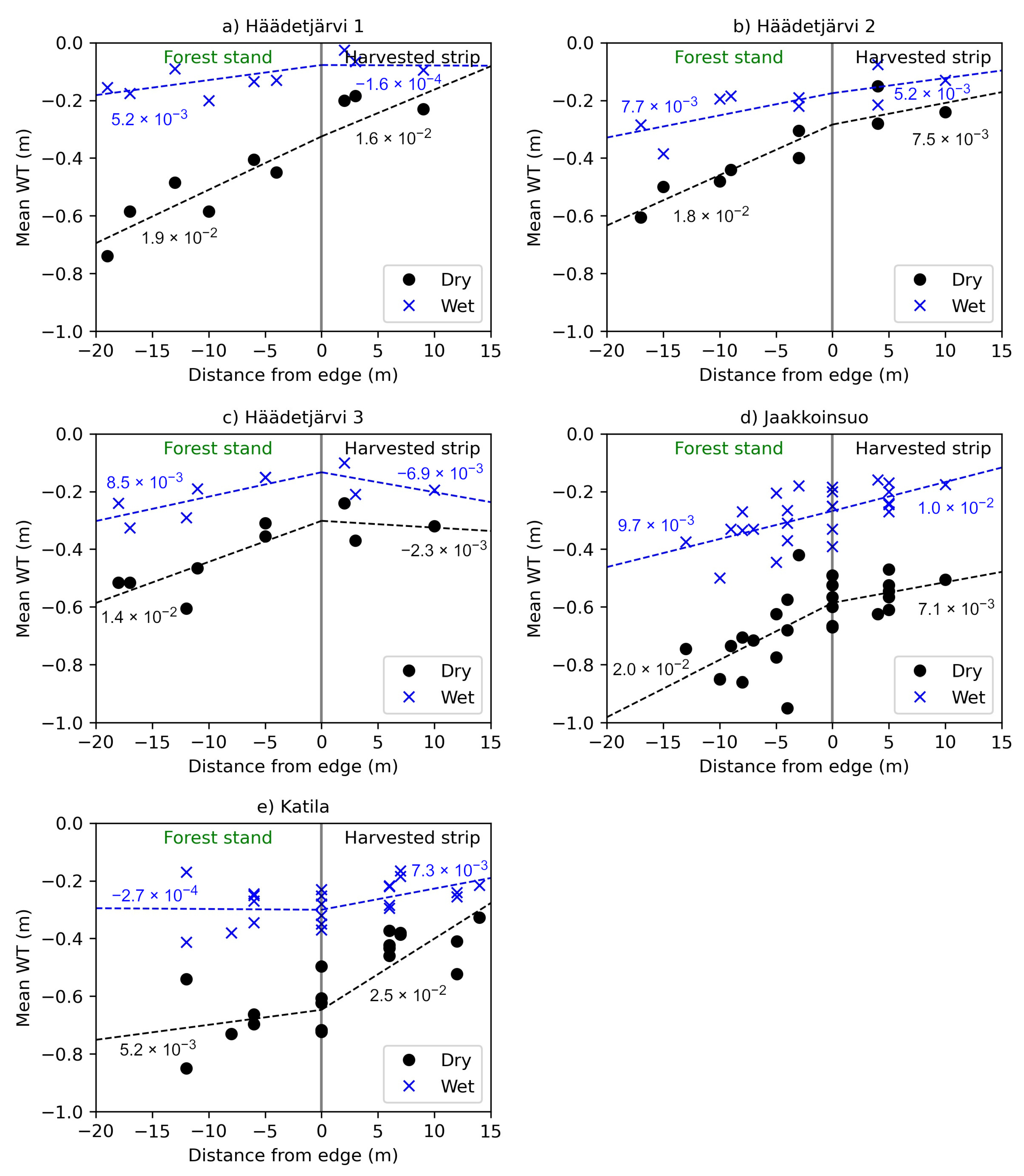
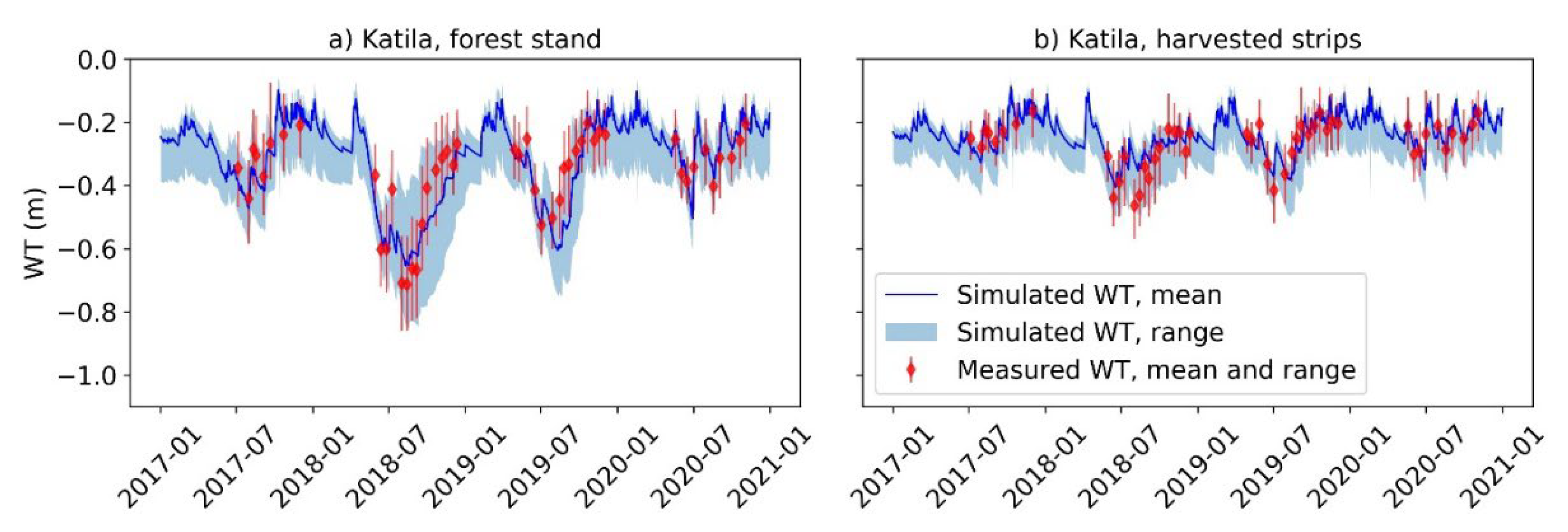
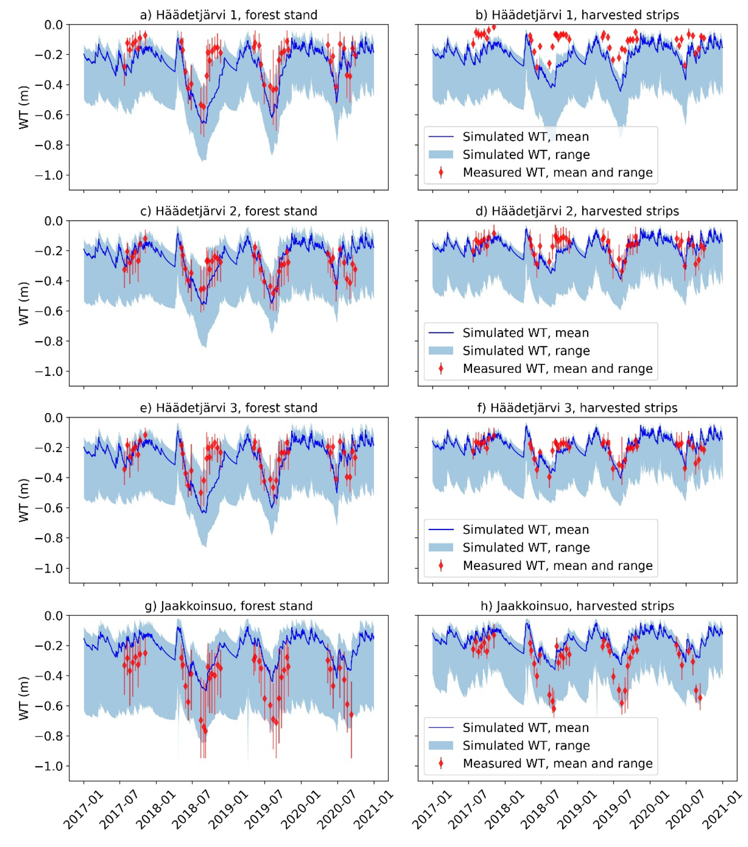
The measured WTs in the strip cut drained peatland forests showed that in the harvested strips, the WTs remained much closer to the surface than in the adjacent unharvested tree stands, especially during dry growing seasons (Figure 3). The WT differences between the strips and unharvested stands produced by the model were of a similar magnitude (Table 3). The larger difference in the observed WTs than in the simulated WTs at the four sites can be explained by the fact that the observed WTs covered only the tube locations, while the simulated WT differences were calculated from the mean WT within the whole unharvested or harvested domains. In one of the sites (i.e., Häädetjärvi 3), the difference in the observed WTs between the unharvested stand and the harvested strip was approximately 50% smaller than the other sites (Table 3). This was most likely related to the better drainage of the harvested strip compared to the other sites (Figure 3a–c). Because the dimensions of the drainage structures were similar, probable explanations include different peat hydraulic properties or field layer vegetation with high ET capacity.
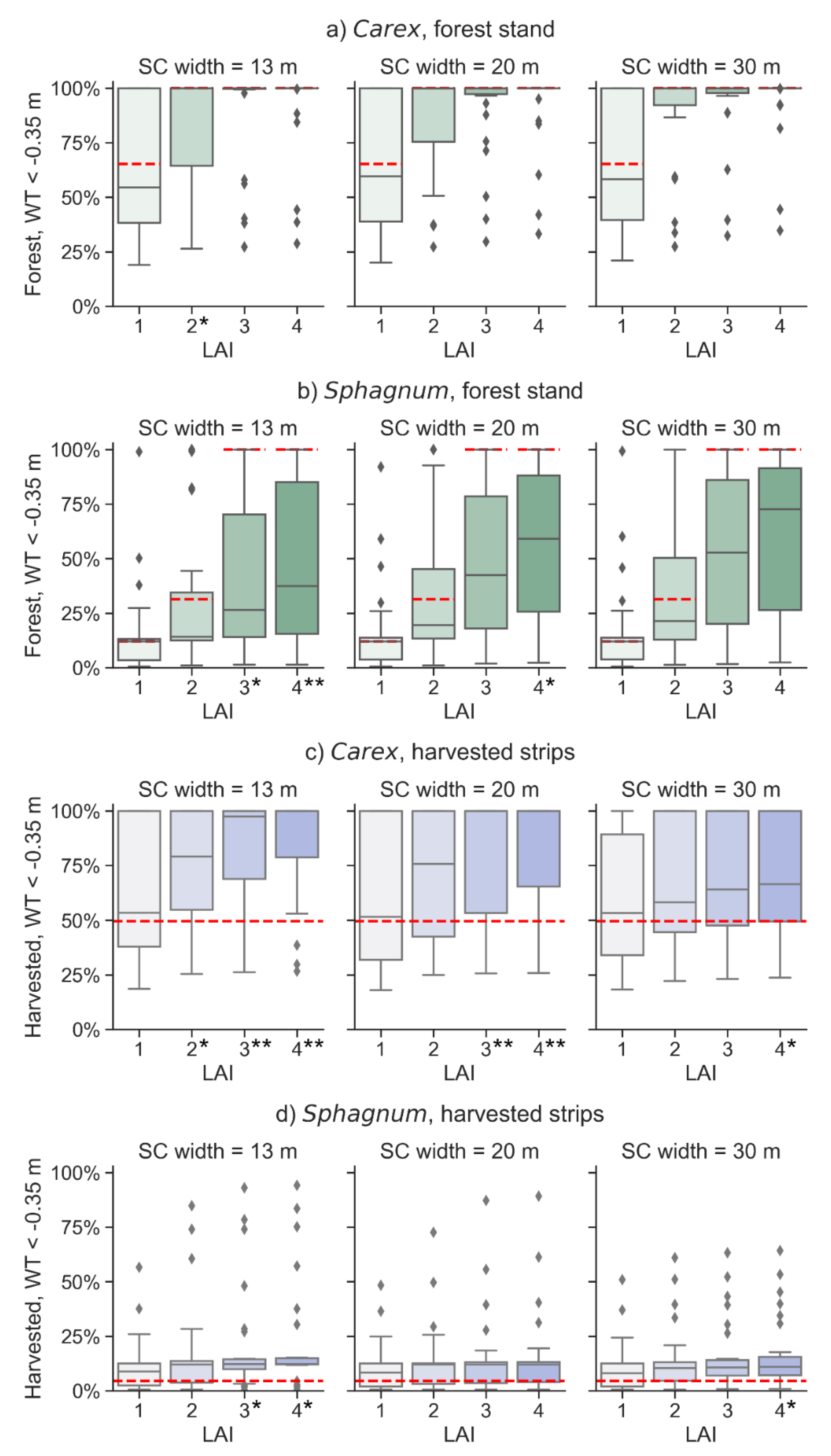
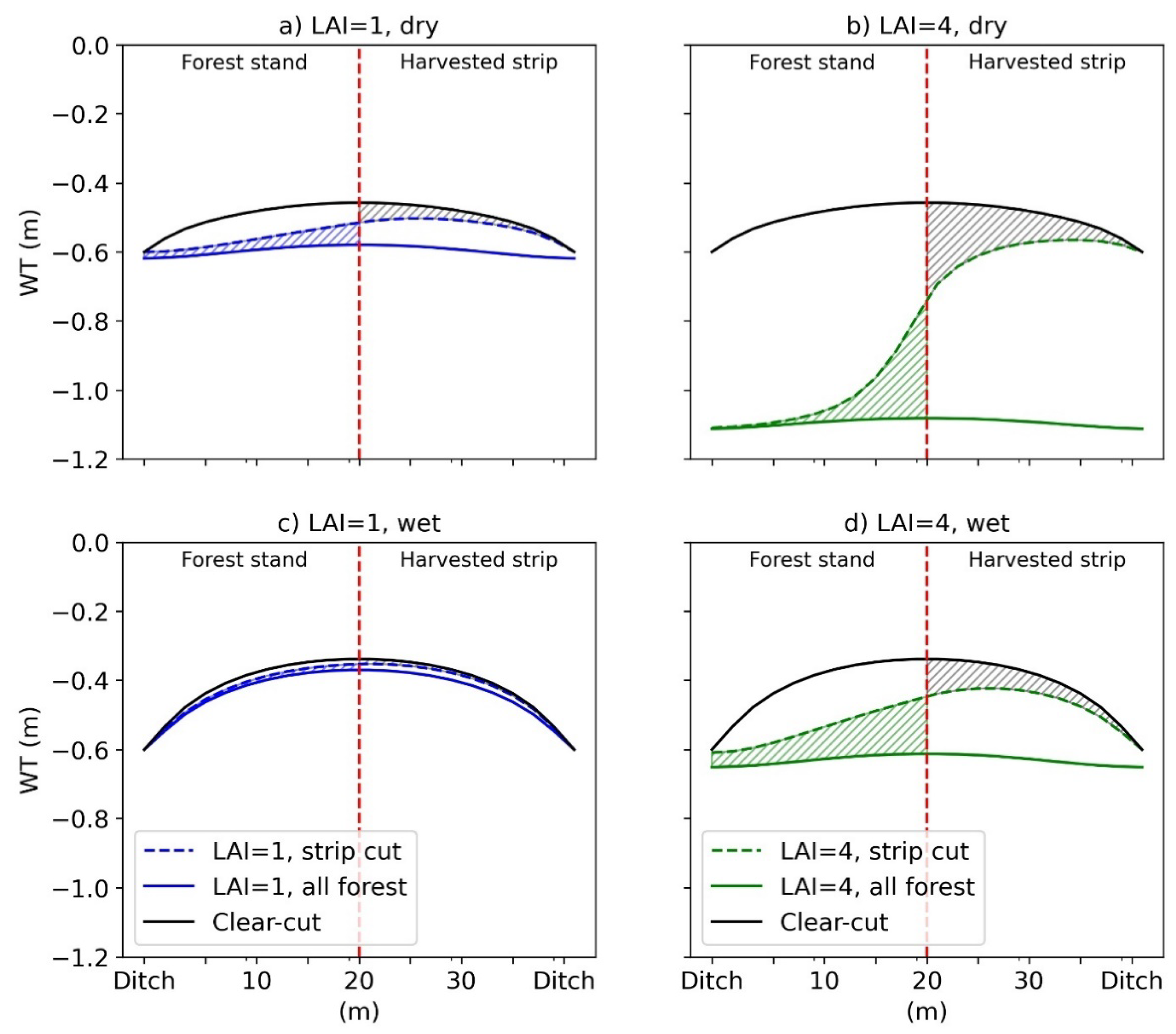
The results suggest strip cutting had limited capacity to keep the WT below the desired −0.35 m level in the harvested strips (Figure 7c–d), especially in wet conditions and in the Sphagnum peat sites. Sphagnum peat had low hydraulic conductivity, and the harvested strips could not be adequately drained, even if the LAI (i.e., the stand volume of the adjacent forest) was large (Figure 7d). However, compared to clear-cutting, strip cutting may be a better alternative. This is especially true when the adjacent stand has an LAI ≥ 2, and the site is characterized by Carex peat with high hydraulic conductivity. In these conditions, strip cutting yielded a notable improvement in the share of the well-drained area compared to clear-cutting (
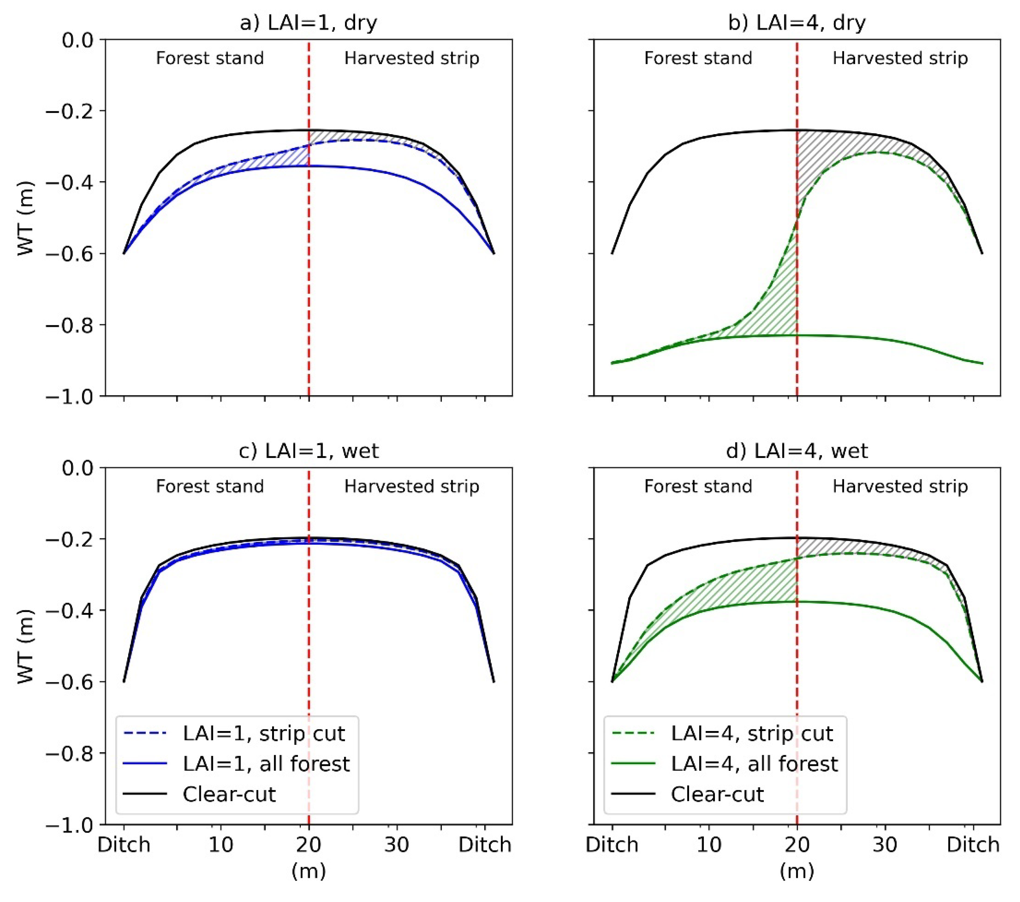
Figure 7c). Narrower strip widths improved drainage on the harvested strips, as the drying effect of the adjacent stand was the highest near the strip edges and faded further away (Figure 6).
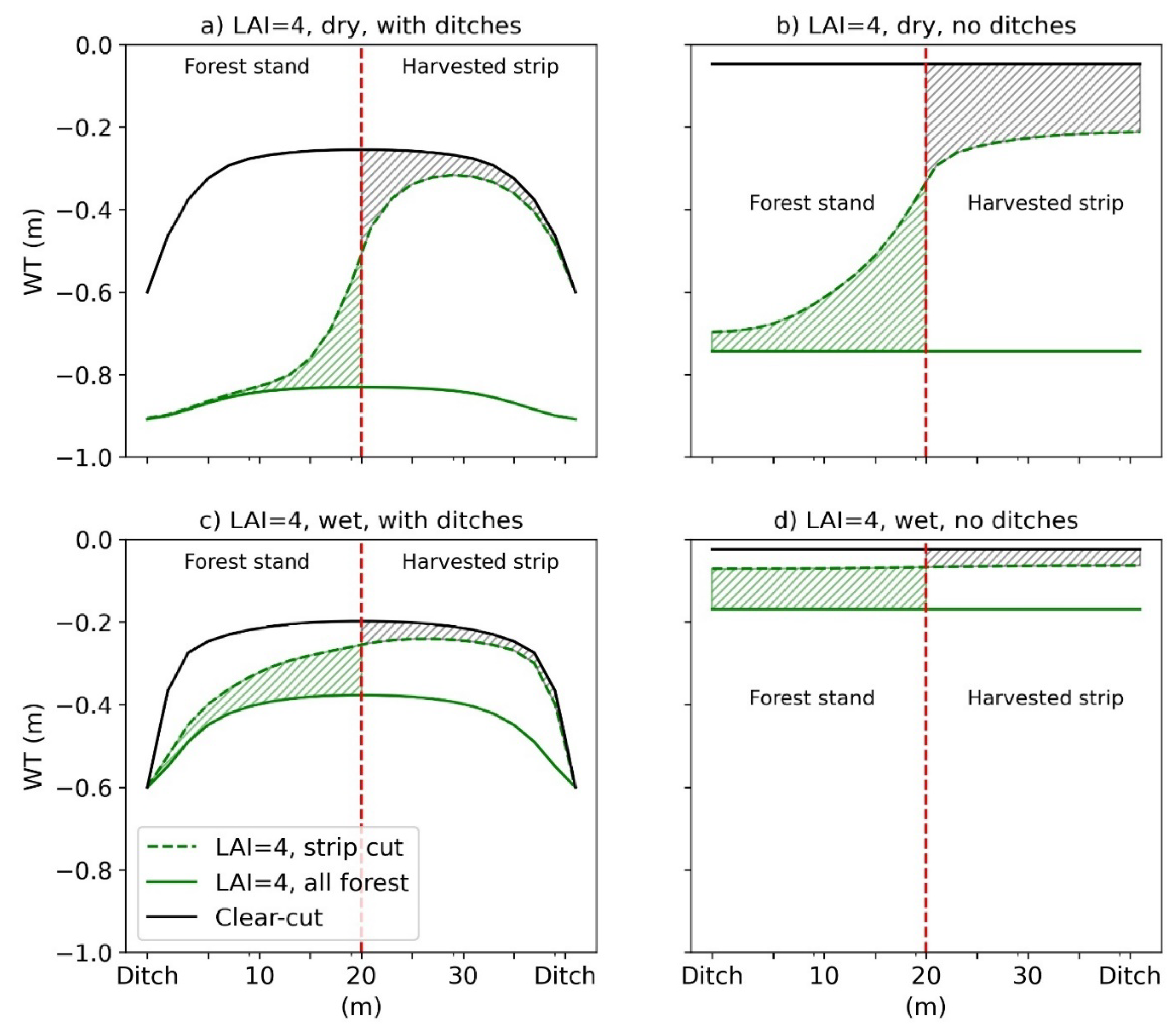
The simulated edge effects in different weather conditions (Figure 6) and the sensitivity analysis (Table 4) jointly indicate that the drainage on the harvested strips was better in southern than northern Finland, and this is mostly related to climatologically driven differences in precipitation and ET. It seems that in northern Finland, forest regeneration with strip cuttings is hydrologically feasible only in Carex peat sites. Similar conclusions have been made also for selection cuttings [12]. However, as the importance of ET in controlling the WT is likely to increase, especially in northern Finland, in the future climate [12], the hydrological feasibility of strip cuttings might increase in future elevated temperatures.
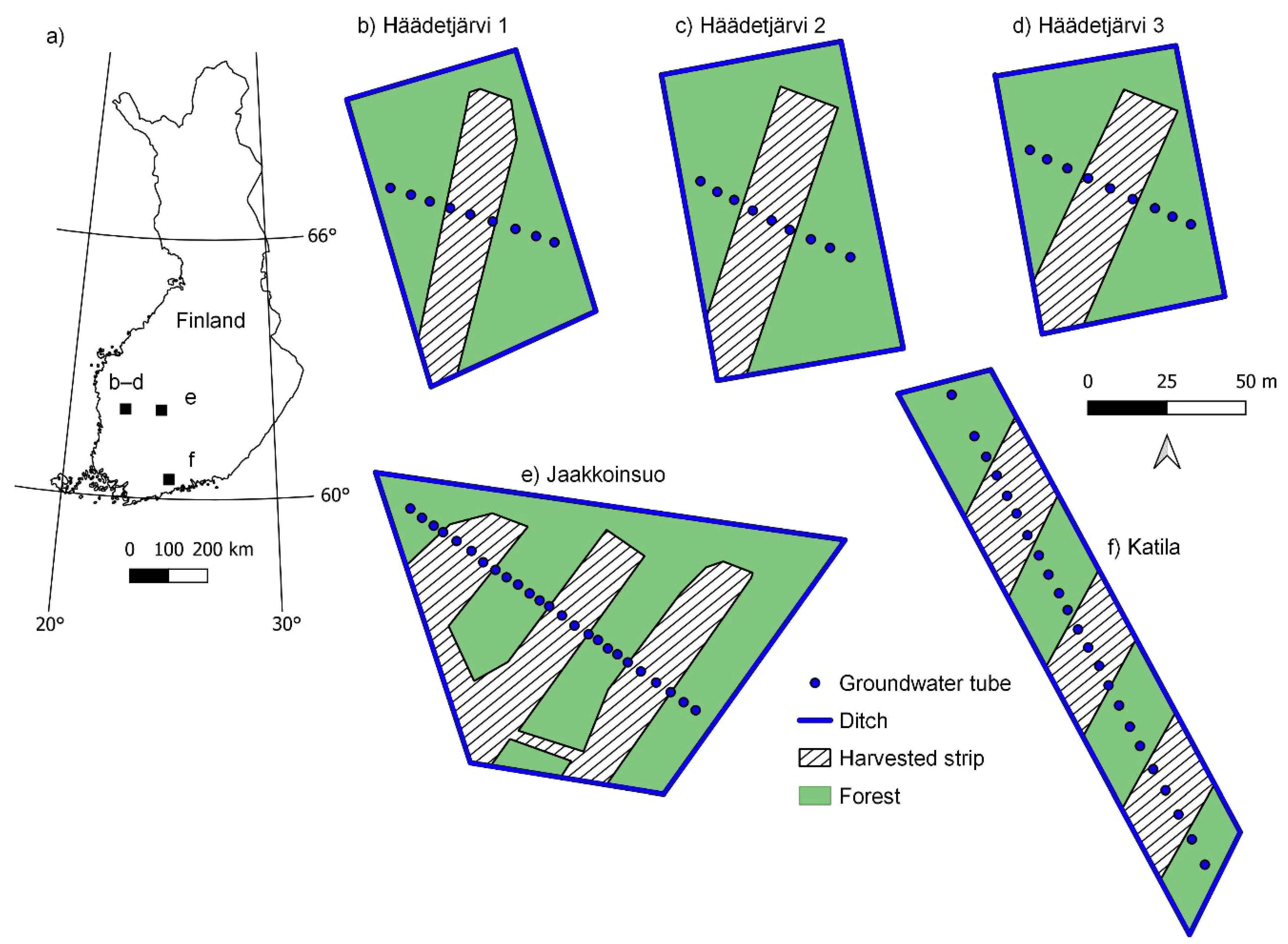
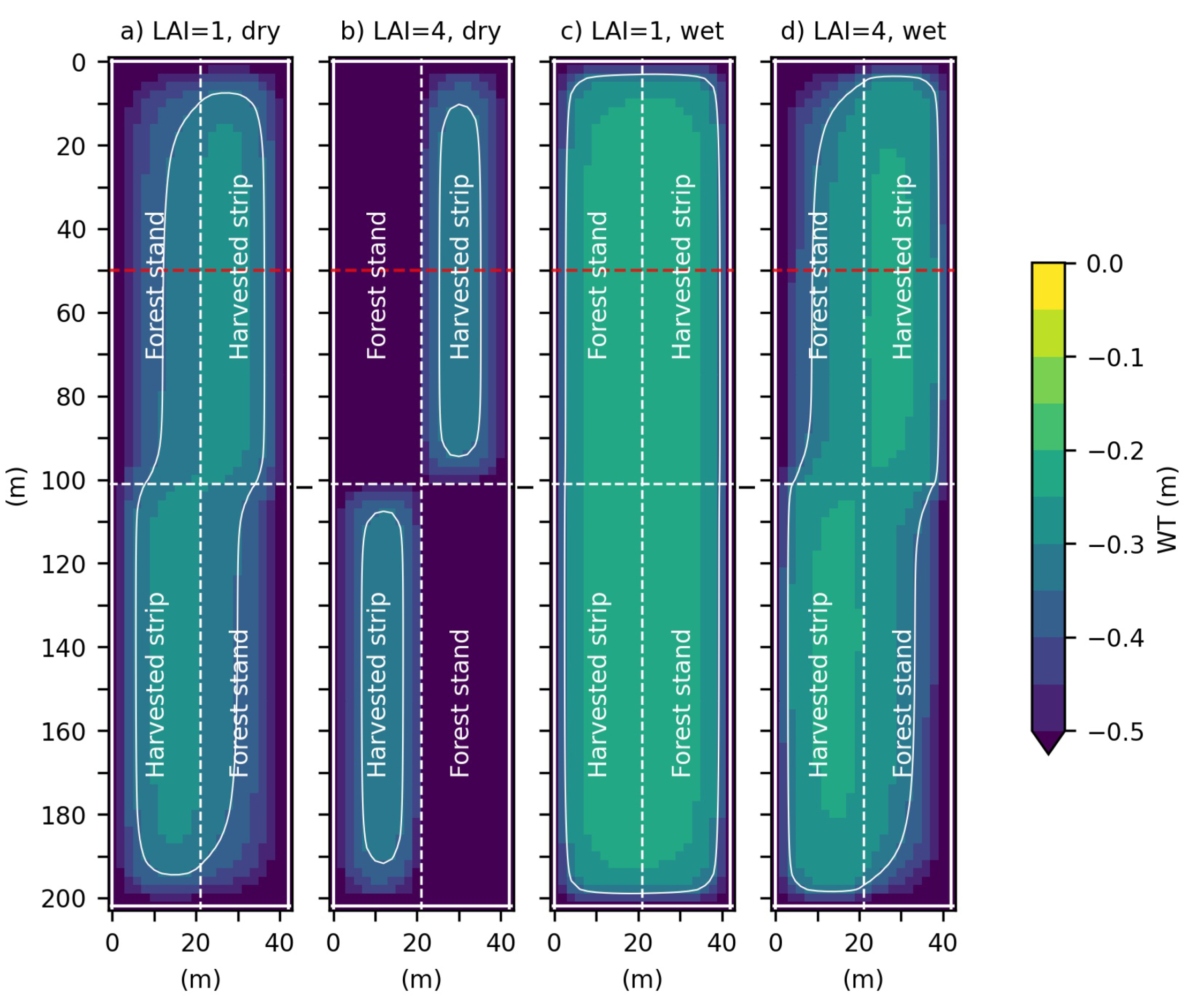
Observed WT data from our experimental sites showed a clear WT gradient between and within unharvested stands and harvested strips in the dry summer conditions (Figure 3). The WTs in the adjacent unharvested stands were clearly lower the farther the distance from the edge of the harvested strips. However, the vicinity of the ditches also affected the WT. This makes it difficult to interpret the edge effects from the observed WT data, because it is not possible to separate them from the drainage effect of the ditches. In the harvested strips, the measured gradient was not as clear as in the adjacent unharvested stands.
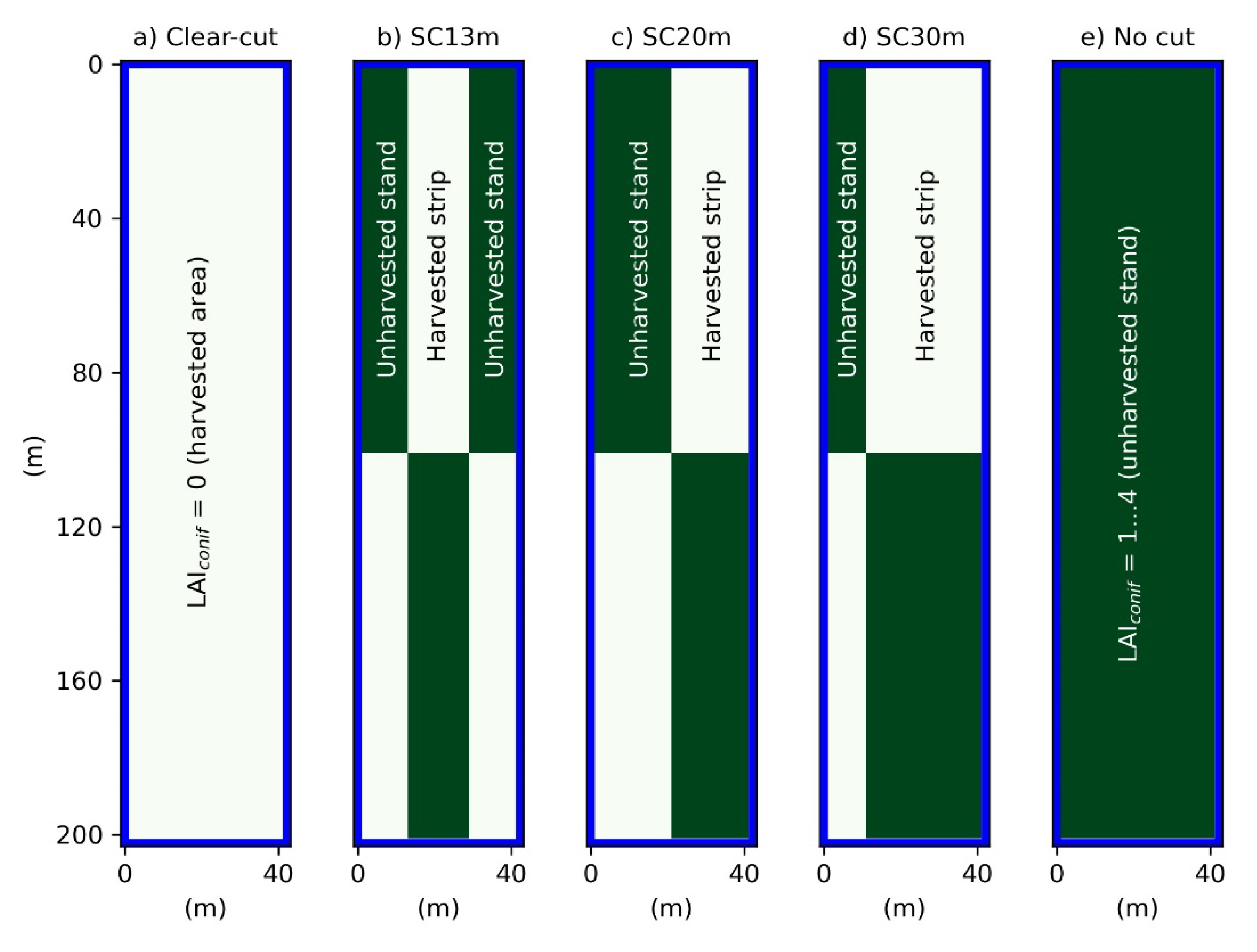
Edge effects were studied by comparing the simulated WT of a strip cut area to the WT in a case where either no cuttings or clear-cutting was applied to the whole area. Edge effects smooth the WT differences between unharvested stands and harvested strips. Simulation results showed that this was most affected by the stand density (Figure 6). Secondary impacts were caused by weather or climate conditions. There were also several other factors affecting the magnitude of the edge effect: distance to ditches, ditch depth, peat hydraulic properties, and strip cut width. The magnitude of the edge effect was strongest in dry conditions. When the soil hydraulic conductivity was low and the water retention capacity was high (such as in Sphagnum peat, Figure 6), the edge effect did not reach as far into the unharvested stands or harvested strips as in the soil with higher hydraulic conductivity (such as Carex peat, Appendix C). Ditch drainage strongly affected the WT near the ditches and, as a result, suppressed the edge effects (see Appendix D for an example). In drained peatlands, the extent of the edge effects depends on the ditch depth and peat hydraulic properties that control ditch drainage.
There is evidence that transpiration can be higher near the forest edge than in the inner forest [34,35]. This could be the result of better water availability [34] or differences in the light environment [35]. However, with Scots pine, the needle mass is thought to explain the variability in transpiration more than the distance and diameter of neighboring trees [36]. In our model, transpiration may be limited by water availability, although in drained peatlands, such dry conditions are rare [37]. Differences in needle mass in edge and inner forests were not accounted for in this study. Higher transpiration near the forest edge caused by different light environments was also not accounted for in the current model structure. Thus, near the forest edge, our model predictions may have yielded WTs that were closer to the surface than if the above effects were accounted for fully.
In addition to hydrology, edge effects also affect stand growth and allometry [38,39] and understory vegetation composition [40]. Trees growing close to the forest edges receive more light and have better access to nutrient resources in the harvested strip. However, WT rise (Figure 7a,b) within the edges of an unharvested stand might also reduce tree growth compared to completely forested peatland with a deeper WT. Forest regeneration in the harvested strip is also affected by the competition inflicted by the surrounding unharvested tree stand. Competition can reduce height growth as far as approximately half of the dominant height of the surrounding forest [3,39]. From the point of view of maintaining satisfactory drainage conditions after harvesting, narrow strips would be optimal, but too narrow strips can be impractical because of higher competition and unfavorable light conditions for seedlings established in the harvested strip. A balance between the WT, vegetation competition, and other factors, such as the direction of the strip in relation to the optimal amount of solar radiation, is thus needed in selecting proper strip cut width.
Strip cutting reduced increases in the WTs of harvested strips and resulted in smaller annual runoff (not shown), especially smaller runoff peaks, compared to clear-cuts. Compared to selection harvestings, WTs in the harvested strips would be higher but runoff would not differ much between the methods if the average stand volumes were similar. Thus, from an environmental point of view, strip cutting can be beneficial compared to clear-cuts, as it may mitigate the export of nutrients and carbon-sensitive anoxic redox reactions [2] as well as have a positive environmental impact by reducing runoff and ditch erosion [41].
In strip cuttings, high water levels will likely occur in parts of the harvested strips and also in the unharvested stands, particularly during wet years. Similarly, WTs will likely drop down to deep peat layers, particularly in forest stands during dry summers. To diminish GHG emissions from drained peatland forests, WTs should be kept at a suitable level, not too high so as to enhance CH4 emissions and not too low so as to increase CO2 and N2O emissions [2,42]. Nevertheless, compared to clear-cut-based forestry, where the entire area will be either completely forested or clear-cut, significantly smaller areas will be subjected to extremely high or low water levels in the strip cut areas. This may decrease both water quality impacts and GHG emissions [2]. Even though strip cutting may not be as effective a means of controlling water levels as selection harvesting [12], more research is still needed to compare the overall environmental and economic effects among the different management types. Strip cutting may be a more feasible management option than selection harvesting, for example, because of the better growth of shade-intolerant tree species and lower forestry harvesting costs.

5. Conclusions

To conclude, both the field trials and model simulations suggested strip cutting of Scots pine-dominated drained peatland can result in a significantly smaller fraction of the harvested strip area with high WT than clear-cuts, which may have environmental benefits. However, the effects of strip cutting on WT and drainage conditions are strongly driven by site and weather conditions. While strip cutting may be a feasible means of controlling WTs at sites with high hydraulic conductivity typical of the medium productive sites in southern Finland, it is not effective in poorly conductive peat soils (typical in nutrient poor sites). It may also be used to control WTs much more effectively in sites with high initial stand density. Narrow strips allowed for better control of WTs than wide strips, but further research is still needed to assess proper strip width from economic and environmental perspectives. In general, it appears that strip cutting is not as effective a means of controlling WTs on drained peatlands as selection harvests. A crucial future research question is how tree stand start to regenerate in a harvested strip, as its contribution to drainage should be considered in the timing of subsequent harvestings in the strip cut area. Future research could also explore strip cut layouts with three or more strips with differently developed stands [43].

Author Contributions

Conceptualization and methodology, all authors; software, A.L., S.L. and K.L.; formal analysis, L.S.; investigation and data curation, M.N., S.S., H.H. and M.S., writing—original draft preparation, L.S., K.L. and S.L.; writing—review and editing, all authors; visualization, L.S.; supervision, M.N. All authors have read and agreed to the published version of the manuscript.

Funding

This research was funded by the Suo-PPP public–private partnership project of the Natural Resources Institute Finland and the Academy of Finland (no. 310203). L.S. acknowledges funding from the Ministry of Agriculture and Forestry of Finland (HYTKY-project). K.L. acknowledges funding from the Academy of Finland (no. 332141). S.L. acknowledges funding from the Academy of Finland (no. 296116). A.L. acknowledges funding from the Academy of Finland (no. 325168).

Institutional Review Board Statement

Not applicable.

Informed Consent Statement

Not applicable.

Data Availability Statement

The datasets generated for this study and the model source code are available upon request from the corresponding author.

Acknowledgments

The authors wish to acknowledge the CSC—IT Center for Science, Finland, for the computational resources.

Conflicts of Interest

The authors declare no conflict of interest.

Appendix A

Table A1. The Sphagnum peat profile’s hydraulic characteristics.
Depth (m)θs (m3 m−3)θr (m3 m−3)αβKsat (m h−1)
0.0–0.10.950.0980.3381.409.71
0.1–0.20.920.0980.0721.372.15
0.2–0.30.920.0980.0721.370.35
0.3–0.40.920.0980.0721.371.2 × 10−2
0.4–0.50.920.0980.0721.373.9 × 10−3
0.5–2.00.920.0980.0721.371.3 × 10−3–4.2 × 10⁻⁴
θs = soil porosity; θr = residual water content; α, β = van Genuchten water retention curve parameters; Ksat = saturated hydraulic conductivity.
Table A2. The Carex peat profile’s hydraulic characteristics.
Depth (m)θs (m3 m−3)θr (m3 m−3)αβKsat (m h−1)
0.0–0.10.940.0020.2021.355.37
0.1–0.20.870.1980.0301.492.31
0.2–0.30.870.1980.0301.490.75
0.3–0.40.870.1980.0301.494.8 × 10−2
0.4–0.50.870.1980.0301.493.1 × 10−2
0.5–2.00.870.1980.0301.492.0 × 10−2–4.2 × 10⁻⁴
θs = soil porosity; θr = residual water content; α, β = van Genuchten water retention curve parameters; Ksat = saturated hydraulic conductivity.

Appendix B

Figure A1. Simulated spatial mean and range of daily WTs in 2017–2020 and measured WTs within unharvested forest stand (a,c,e,g) and harvested (treeless) strips (b,d,f,h) at the study site. Measurement data from tubes located at the edge of forests and harvested strips were omitted. The simulated WTs’ ranges covered the whole forest or harvested area.
Forests 13 01134 g0a1

Appendix C

Figure A2. Cross-sectional (y = 50 m in Figure 5), momentary simulated WTs at the end of August during a dry summer (a,b) and a wet summer (c,d) in Carex peat areas with a −0.6 m ditch depth, LAI = 1, and LAI = 4. The edge between the forest and harvested strips is separated by the red, dashed lines. The blue (LAI = 1) and green (LAI = 4) hatched areas indicate the edge effects of the harvested strip on the forest stand. The gray hatched areas indicate edge effects of the forest stand on the harvested strip.
Forests 13 01134 g0a2

Appendix D

Figure A3. Cross-sectional, momentary simulated WT at the end of August during a dry (a,b) and wet (c,d) growing season in a Sphagnum peat area with ditches (depth: −0.6 m) (a,c) and without ditches (b,d). The edge between the forest stand and the harvested strip is separated with red, dashed lines. Green hatched areas indicate the edge effect of the harvested strip on the forest stand. The gray hatched areas indicate the edge effect of the forest stand on the harvested strip.
Forests 13 01134 g0a3

References

  1. Päivänen, J.; Hånell, B. Peatland Ecology and Forestry—A Sound Approach; University of Helsinki, Department of Forest Sciences Publications 3: Helsinki, Finland, 2012. [Google Scholar]
  2. Nieminen, M.; Hökkä, H.; Laiho, R.; Juutinen, A.; Ahtikoski, A.; Pearson, M.; Kojola, S.; Sarkkola, S.; Launiainen, S.; Valkonen, S.; et al. Could continuous cover forestry be an economically and environmentally feasible management option on drained boreal peatlands? For. Ecol. Manag. 2018, 424, 78–84. [Google Scholar] [CrossRef]
  3. Ahtikoski, A.; Hökkä, H.; Siipilehto, J. Strip cutting management in Scots pine stands on peatlands—A financial comparison to rotation forestry. Scan. J. For. Res. 2022, 37, 119–129. [Google Scholar] [CrossRef]
  4. Juutinen, A.; Shanin, V.; Ahtikoski, A.; Rämö, J.; Mäkipää, R.; Laiho, R.; Sarkkola, S.; Laurén, A.; Penttilä, T.; Hökkä, H.; et al. Profitability of continuous cover forestry in Norway spruce-dominated peatland forest and the role of water table. Can. J. For. Res. 2020, 51, 859–870. [Google Scholar] [CrossRef]
  5. Leemans, R. Canopy gaps and establishment patterns of spruce (Picea abies (L.) Karst.) in two old-growth coniferous forests in central Sweden. Vegetatio 1991, 93, 157–165. [Google Scholar] [CrossRef]
  6. Sarkkola, S.; Hökkä, H.; Ahti, E.; Nieminen, M.; Koivusalo, H. Depth of water table prior to ditch network maintenance is a key factor for tree growth response. Scan. J. For. Res. 2012, 27, 649–658. [Google Scholar] [CrossRef]
  7. Hökkä, H.; Laurén, A.; Stenberg, L.; Launiainen, S.; Leppä, K.; Nieminen, M. Defining guidelines for ditch depth in drained Scots pine dominated peatland forests. Silva Fennica 2021, 55, 10494. [Google Scholar] [CrossRef]
  8. Saarinen, M.; Alenius, V.; Laiho, R. Effect of soil moisture conditions on seed germination and early seedling development in prepared microsites in peatland forest regeneration areas. Suo 2013, 64, 51–75. Available online: http://www.suo.fi/pdf/article9887.pdf (accessed on 4 July 2022). (In Finnish with English summary).
  9. Ojanen, P.; Minkkinen, K.; Alm, J.; Penttilä, T. Soil-atmosphere CO2, CH4 and N2O fluxes in boreal forestry-drained peatlands. For. Ecol. Manag. 2010, 260, 411–421. [Google Scholar] [CrossRef]
  10. Korkiakoski, M.; Tuovinen, J.-P.; Penttilä, T.; Sarkkola, S.; Ojanen, P.; Minkkinen, K.; Rainne, J.; Laurila, T.; Lohila, A. Greenhouse gas and energy fluxes in a boreal peatland forest after clear-cutting. Biogeosciences 2019, 16, 3703–3723. [Google Scholar] [CrossRef] [Green Version]
  11. Kaila, A.; Asam, Z.; Koskinen, M.; Uusitalo, R.; Smolander, A.; Kiikkilä, O.; Sarkkola, S.; O’Driscoll, C.; Kitunen, V.; Fritze, H.; et al. Impact of re-wetting of forestry-drained peatlands on water quality–a laboratory approach assessing the release of P, N, Fe, and dissolved organic carbon. Water Air Soil Pollut. 2016, 227, 292. [Google Scholar] [CrossRef]
  12. Leppä, K.; Hökkä, H.; Laiho, R.; Launiainen, S.; Lehtonen, A.; Mäkipää, R.; Peltoniemi, M.; Saarinen, M.; Sarkkola, S.; Nieminen, M. Selection Cuttings as a Tool to Control Water Table Level in Boreal Drained Peatland Forests. Front. Earth Sci. 2020, 8, 576510. [Google Scholar] [CrossRef]
  13. Sarkkola, S.; Hökkä, H.; Koivusalo, H.; Nieminen, M.; Ahti, E.; Päivänen, J.; Laine, J. Role of tree stand evapotranspiration in maintaining satisfactory drainage conditions in drained peatlands. Can. J. For. Res. 2010, 40, 1485–1496. [Google Scholar] [CrossRef]
  14. Laurén, A.; Palviainen, M.; Launiainen, S.; Leppä, K.; Stenberg, L.; Urzainki, I.; Nieminen, M.; Laiho, R.; Hökkä, H. Drainage and Stand Growth Response in Peatland Forests—Description, Testing, and Application of Mechanistic Peatland Simulator SUSI. Forests 2021, 12, 293. [Google Scholar] [CrossRef]
  15. Haahti, K.; Koivusalo, H.; Hökkä, H.; Nieminen, M.; Sarkkola, S. Factors affecting the spatial variability of water table depth within a drained peatland forest in northern Finland. Suo 2012, 63, 107–121. Available online: http://www.suo.fi/pdf/article9883.pdf (accessed on 4 July 2022). (In Finnish with English summary).
  16. Hökkä, H.; Uusitalo, J.; Lindeman, H.; Ala-Ilomäki, H. Performance of weather parameters in predicting growing season water table depth variations on drained forested peatlands—A case study from southern Finland. Silva Fennica 2016, 50, 1687. [Google Scholar] [CrossRef] [Green Version]
  17. Stenberg, L.; Haahti, K.; Hökkä, H.; Launiainen, S.; Nieminen, M.; Laurén, A.; Koivusalo, H. Hydrology of Drained Peatland Forest: Numerical Experiment on the Role of Tree Stand Heterogeneity and Management. Forests 2018, 9, 645. [Google Scholar] [CrossRef] [Green Version]
  18. Kubota, T.; Kagawa, A.; Abe, T.; Hosoda, I. Effects of clear-cutting, meteorological, and physiological factors on evapo-transpiration in the Kamabuchi experimental watershed in northern Japan. Hydrol. Processes 2021, 35, e14111. [Google Scholar] [CrossRef]
  19. Kozii, N.; Haahti, K.; Tor-ngern, P.; Chi, J.; Hasselquist, E.M.; Laudon, H.; Launiainen, S.; Oren, R.; Peichl, M.; Wallerman, J.; et al. Partitioning growing season water balance within a forested boreal catchment using sap flux, eddy covariance, and a process-based model. Hydrol. Earth Syst. Sci. 2020, 24, 2999–3014. [Google Scholar] [CrossRef]
  20. Leppä, K.; Korkiakoski, M.; Nieminen, M.; Laiho, R.; Hotanen, J.-P.; Kieloaho, A.-J.; Korpela, L.; Laurila, T.; Lohila, A.; Minkkinen, K.; et al. Vegetation controls of water and energy balance of a drained peatland forest: Responses to alternative harvesting practices. Agric. For. Meteorol. 2020, 295, 108198. [Google Scholar] [CrossRef]
  21. Sadeghi, S.M.M.; Gordon, D.A.; Van Stan, J.T., II. A Global Synthesis of Throughfall and Stemflow Hydrometeorology. In Precipitation Partitioning by Vegetation: A Global Synthesis; Van Stan, J.T., II, Gutmann, E., Friesen, J., Eds.; Springer International Publishing: Cham, Switzerland, 2020; pp. 49–70. [Google Scholar] [CrossRef]
  22. Launiainen, S.; Guan, M.; Salmivaara, A.; Kieloaho, A.-J. Modeling boreal forest evapotranspiration and water balance at stand and catchment scales: A spatial approach. Hydrol. Earth Syst. Sci. 2019, 23, 3457–3480. [Google Scholar] [CrossRef] [Green Version]
  23. Urzainki, I.; Laurén, A.; Palviainen, M.; Haahti, K.; Budiman, A.; Basuki, I.; Netzer, M.; Hökkä, H. Canal blocking optimization in restoration of drained peatlands. Biogeosciences 2020, 17, 4769–4784. [Google Scholar] [CrossRef]
  24. Vasander, H.; Laine, J. Site Type Classification on Drained Peatlands. In Finland—Fenland: Research and Sustainable Utilisation of Mires and Peat; Korhonen, R., Korpela, L., Sarkkola, S., Eds.; Finnish Peatland Society, Maahenki Ltd.: Helsinki, Finland, 2008; pp. 146–151. [Google Scholar]
  25. Päivänen, J. Hydraulic conductivity and water retention in peat soils. Acta For. Fenn. 1973, 129, 1–70. [Google Scholar] [CrossRef] [Green Version]
  26. Aalto, J.; Pirinen, P.; Heikkinen, J.; Venäläinen, A. Spatial interpolation of monthly climate data for Finland: Comparing the performance of kriging and generalized additive models. Theor. Appl. Climatol. 2013, 112, 99–111. [Google Scholar] [CrossRef]
  27. Ťupek, B.; Mäkipää, R.; Heikkinen, J.; Peltoniemi, M.; Ukonmaanaho, L.; Hokkanen, T.; Nöjd, P.; Nevalainen, S.; Lindgren, M.; Lehtonen, A. Foliar turnover rates in Finland—Comparing estimates from needle-cohort and litterfall-biomass methods. Boreal Environ. Res. 2015, 20, 283–304. Available online: http://hdl.handle.net/10138/228149 (accessed on 4 July 2022).
  28. Lehtonen, A.; Heikkinen, J.; Petersson, H.; Ťupek, B.; Liski, E.; Mäkelä, A. Scots pine and Norway spruce foliage biomass in Finland and Sweden—Testing traditional models vs. the pipe model theory. Can. J. For. Res. 2020, 50, 146–154. [Google Scholar] [CrossRef]
  29. Härkönen, S.; Lehtonen, A.; Manninen, T.; Tuominen, S.; Peltoniemi, M. Estimating forest leaf area index using satellite images: Comparison of k-NN based Landsat-NFI LAI with MODIS-RSR based LAI product for Finland. Boreal Environ. Res. 2015, 20, 181–195. [Google Scholar]
  30. Korhonen, L.; Korhonen, K.T.; Stenberg, P.; Maltamo, M.; Rautiainen, M. Local models for forest canopy cover with beta regression. Silva Fennica 2007, 41, 671–685. [Google Scholar] [CrossRef] [Green Version]
  31. Cermák, J.; Riguzzi, F.; Ceulemans, R. Scaling up from the individual tree to the stand level in Scots pine. I. Needle distribution, overall crown and root geometry. Ann. For. Sci. 1998, 55, 63–88. [Google Scholar] [CrossRef] [Green Version]
  32. Nagel, J.; Albert, M.; Schmidt, M. Das waldbauliche Prognose-und Entscheidungsmodell BWINPro 6.1. Forst Holz 2002, 57, 486–493. [Google Scholar]
  33. Venäläinen, A.; Tuomenvirta, H.; Pirinen, P.; Drebs, A. A Basic Finnish Climate Data Set 1961–2000—Description and Illustrations; Reports 2005:5; Finnish Meteorological Institute: Helsinki, Finland. [CrossRef]
  34. Cienciala, E.; Mellander, P.-E.; Kučera, J.; Opluštilová, M.; Ottosson-Löfvenius, M.; Bishop, K. The effect of a north-facing forest edge on tree water use in a boreal Scots pine stand. Can. J. For. Res. 2002, 32, 693–702. [Google Scholar] [CrossRef]
  35. Ringgaard, R.; Herbst, M.; Friborg, T. Partitioning of forest evapotranspiration: The impact of edge effects and canopy structure. Agric. For. Meteorol. 2012, 166–167, 86–97. [Google Scholar] [CrossRef]
  36. Lagergren, F.; Lindroth, A. Variation in sapflow and stem growth in relation to tree size, competition and thinning in a mixed forest of pine and spruce in Sweden. For. Ecol. Manage. 2004, 188, 51–63. [Google Scholar] [CrossRef]
  37. Schwärzel, K.; Šimumek, J.; van Genuchten, M.T.; Wessolek, G. Measurement and modeling of soil-water dynamics and evapotranspiration of drained peatland soils. J. Plant Nutr. Soil Sci. 2006, 169, 762–774. [Google Scholar] [CrossRef]
  38. Nikolova, P.S.; Geyer, J.; Brang, P.; Cherubini, P.; Zimmermann, S.; Gärtner, H. Changes in Root-Shoot Allometric Relations in Alpine Norway Spruce Trees After Strip Cutting. Front. Plant Sci. 2021, 12, 703674. [Google Scholar] [CrossRef]
  39. Siipilehto, J. Height Distributions of Scots Pine Sapling Stands Affected by Retained Tree and Edge Stand Competition. Silva Fennica 2006, 40, 331. [Google Scholar] [CrossRef] [Green Version]
  40. Alignier, A.; Deconchat, M. Patterns of forest vegetation responses to edge effect as revealed by a continuous approach. Ann. For. Sci. 2013, 70, 601–609. [Google Scholar] [CrossRef] [Green Version]
  41. Stenberg, L.; Tuukkanen, T.; Finér, L.; Marttila, H.; Piirainen, S.; Kløve, B.; Koivusalo, H. Ditch erosion processes and sediment transport in a drained peatland forest. Ecol. Eng. 2015, 75, 421–433. [Google Scholar] [CrossRef]
  42. Ojanen, P.; Minkkinen, K. The dependence of net soil CO2 emissions on water table depth in boreal peatlands drained for forestry. Mires Peat 2019, 24, 1–8. [Google Scholar] [CrossRef]
  43. Saarinen, M.; Valkonen, S.; Sarkkola, S.; Nieminen, M.; Penttilä, T.; Laiho, R. Jatkuvapeitteisen metsänkasvatuksen mahdollisuudet ojitetuilla turvemailla. Metsätieteen Aikakauskirja (In Finnish). 2020, 10372. [Google Scholar] [CrossRef]
Figure 1. Locations of the study sites within Finland (a) and detailed maps of the strip cuttings (bf) with groundwater tubes on the drained nutrient-poor forested peatlands. The stands are dominated by Scots pine.
Forests 13 01134 g001
Figure 2. Tree stand layouts (ae) tested in the study. The leaf area index (LAIconif, one sided) in the area of the standing trees varied between 1 and 4. There were no trees in the harvested strips. The strip cut (SC) layouts (bd) are named according to strip width (i.e., 13, 20, and 30 m). The blue lines indicate ditches surrounding the areas.
Forests 13 01134 g002
Figure 3. The mean measured WTs in August 2017 (wet, i.e., rainy and cool growing season) and 2018 (dry and warm growing season) at the study sites (ae) in southern Finland according to the WT tube’s location from the edge of the unharvested forest stand and harvested (treeless) strip. Dashed lines present a piecewise linear function (WT − WTedge = ax, where x is the distance from the edge; WTedge is the mean WT at the edge or the nearest points) fitted to the data separately for the forest and harvested strips. The numbers next to the dashed lines represent the slopes of the fitted lines.
Forests 13 01134 g003
Figure 4. The simulated spatial mean and range of the daily WTs in 2017–2020 and the measured WTs within the unharvested forest stand (a) and the harvested (treeless) strips (b) at the Katila study site. Measurement data from tubes located at the edge of the forest and the harvested strips were omitted from this figure. The simulated WTs’ range covered the whole forest and harvested areas.
Forests 13 01134 g004
Figure 5. Snapshots of simulated WTs in a single day at the end of August in dry (a,b) and wet growing seasons (c,d). White contour lines (ad) represent the isolines for a WT = −0.35 m. Unharvested stands and harvested (treeless) strips are separated by dashed, white lines. The peat profile was set to Sphagnum, and the ditch depth at the outer boundaries was equal to −0.6 m. Red, dashed lines indicate the location of the cross-sections presented in Figure 6.
Forests 13 01134 g005
Figure 6. Cross-sections of (y = 50 m in Figure 5) the simulated WTs at the end of August during a dry (a,b) and wet growing season (c,d). The edge between the unharvested stands and the harvested (treeless) strips is shown by the red, dashed line. The blue (LAI = 1) and green (LAI = 4) hatched areas indicate the edge effect of the harvested strip on the adjacent unharvested stand. The gray hatched areas indicate the edge effect of the adjacent unharvested stand on the harvested strip. Sphagnum peat and a −0.6 m ditch depth were assumed.
Forests 13 01134 g006
Figure 7. The simulated share of well-drained areas (WT <−0.35 m during July–August) with Carex peat (a,c) and Sphagnum peat (b,d) for unharvested forest stands (a,b) and harvested (treeless) strips (c,d). In (c,d), the LAI indicate the LAI of the surrounding forest area. The box plots represent between-year variations over 30 years. The dashed, red lines indicate the median for the stands with no harvesting (a,b) or the median for the clear-cut (c,d). The ditch depth was −0.6 m in all simulations. SC width refers to the width of the harvested strip. For tree stand layouts, see Figure 2. In all cases, the shortest distance between ditches was 40 m. For forest stands (a,b), statistically significant differences (* p-value < 0.05; ** p-value < 0.01) were noted comparing the strip cut stands to the stands with no harvesting. For harvested strips, statistically significant differences were noted compared to clear-cuts.
Forests 13 01134 g007
Table 1. Characteristics of the study sites. Tree stand characteristics refer to the adjacent unharvested stand. The standard deviation is presented in parenthesis. BA = stand basal area; Ntubes = number of manual water table measurement points; LAI = average leaf area index (one sided) of coniferous (LAIconif) or deciduous (LAIdecid) tree species after harvesting; tree height = arithmetic mean height of the tree stand in the unharvested stand; DBH = arithmetic mean of the diameters at breast height.
Study SiteLatitudeLongitudeDitch Depth 1Area (ha)BA (m2 ha−1)NtubesLAIconifLAIdecid 2Tree Height (m)DBH (cm)
Häädetjärvi 162°02′13″22°43′18″0.6 m0.5217.093.2 (3.0)0.7 (1.1)15.1 (3.5)18.6 (5.7)
Häädetjärvi 262°02′8″22°43′21″0.6 m0.5316.392.2 (3.1)0.6 (1.1)17.9 (3.4)20.5 (6.4)
Häädetjärvi 362°02′2″22°43′24″0.6 m0.4619.892.8 (2.9)0.5 (0.7)19.7 (1.5)24.5 (3.8)
Jaakkoinsuo62°03′7″24°28′58″0.7 m0.8912.0251.9 (2.6)0.5 (0)17.2 (1.3)18.0 (3.7)
Katila60°27′21″24°57′18″0.4 m0.549.6222.2 (0.4)0.5 (0)20.6 (0.1)25.2 (4.5)
1 Parameter value for simulations. 2 Including deciduous trees’ LAI and an additional 0.5 for field layer vegetation. There were no deciduous trees in Jaakkoinsuo and Katila.
Table 2. Stand parameter combinations used in the simulations. LAIdecid (one sided) was applied in the harvested treeless areas to account for the field layer vegetation. Canopy closure is the value for the unharvested forest stand (see Figure 2b–d) or completely forested layouts (see Figure 2e). In the case of LAIconif = 0 (harvested treeless strip or clear-cut area), dominant height (Hdom) and canopy closure (fc) describe those of the field layer vegetation.
LAIconif (m2 m−2)LAIdecid (m2 m−2)Hdom (m)fc (−)
00.50.50.10
10.5160.40
20.5160.55
30.5160.58
40.5160.62
Table 3. Mean difference in the daily WTs between harvested strips and unharvested stands in May–November 2017–2020. Diffobs and Diffmod refer to observed and simulated differences, respectively. Groundwater tubes located at the edges of the strips were not included in the figures. The average mean absolute errors (MAEs) and root mean square error (RMSE) for the simulated WTs are also presented for the study areas. The standard deviation for each mean value is presented in parenthesis. Ntubes refer to the total number of tubes.
Study SiteDiffobs (m)Diffmod (m)MAE (m)RMSE (m)Ntubes
Häädetjärvi 10.12 (0.08)0.10 (0.07)0.09 (0.03)0.12 (0.04)9
Häädetjärvi 20.12 (0.04)0.09 (0.06)0.08 (0.03)0.09 (0.03)9
Häädetjärvi 30.06 (0.05)0.11 (0.08)0.10 (0.04)0.13 (0.05)9
Jaakkoinsuo0.12 (0.03)0.06 (0.03)0.18 (0.08)0.21 (0.07)25
Katila0.10 (0.07)0.11 (0.09)0.08 (0.03)0.10 (0.04)22
Table 4. Mean July–August WTs over 30 years with different parameter combinations. Unless stated otherwise, the simulation location was Parkano, the ditch depth was −0.6 m, and the LAIdecid was 0.5 (in the harvested strips, describing field layer vegetation). Harvested strips (width: 20 m) covered 50% of the area. For tree stand layout, see Figure 2c.
Carex PeatSphagnum Peat
LAIdecidLAIconif = 1LAIconif = 4LAIconif = 1LAIconif = 4
0.4−0.39−0.50−0.24−0.33
0.5−0.40−0.51−0.25−0.33
0.6−0.41−0.51−0.25−0.34
LocationLAIconif = 1LAIconif = 4LAIconif = 1LAIconif = 4
Nurmijärvi (60°27′ N)−0.46−0.62−0.29−0.42
Parkano (62°02′ N)−0.40−0.51−0.25−0.33
Rovaniemi (66°40′ N)−0.39−0.46−0.24−0.29
Ditch depth (m)LAIconif = 1LAIconif = 4LAIconif = 1LAIconif = 4
−0.48−0.35−0.45−0.24−0.32
−0.60−0.40−0.51−0.25−0.33
−0.72−0.44−0.54−0.26−0.35
Publisher’s Note: MDPI stays neutral with regard to jurisdictional claims in published maps and institutional affiliations.

